Matrix Graph Grammars with Application Conditions

Abstract

In the Matrix approach to graph transformation we represent simple digraphs and rules with Boolean matrices and vectors, and the rewriting is expressed using Boolean operators only. In previous works, we developed analysis techniques enabling the study of the applicability of rule sequences, their independence, state reachability and the minimal graph able to fire a sequence.

In the present paper we improve our framework in two ways. First, we make explicit (in the form of a Boolean matrix) some negative implicit information in rules. This matrix (called nihilation matrix) contains the elements that, if present, forbid the application of the rule (i.e. potential dangling edges, or newly added edges, which cannot be already present in the simple digraph). Second, we introduce a novel notion of application condition, which combines graph diagrams together with monadic second order logic. This allows for more flexibility and expressivity than previous approaches, as well as more concise conditions in certain cases. We demonstrate that these application conditions can be embedded into rules (i.e. in the left hand side and the nihilation matrix), and show that the applicability of a rule with arbitrary application conditions is equivalent to the applicability of a sequence of plain rules without application conditions. Therefore, the analysis of the former is equivalent to the analysis of the latter, showing that in our framework no additional results are needed for the study of application conditions. Moreover, all analysis techniques of [21, 22] for the study of sequences can be applied to application conditions.

Matrix Graph Grammars

Keywords: Graph Transformation, Matrix Graph Grammars, Application Conditions, Monadic Second Order Logic, Graph Dynamics.

1 Introduction

Graph transformation [8, 32] is becoming increasingly popular in order to describe system behaviour due to its graphical, declarative and formal nature. For example, it has been used to describe the operational semantics of Domain Specific Visual Languages (DSVLs) [19], taking the advantage that it is possible to use the concrete syntax of the DSVL in the rules, which then become more intuitive to the designer.

The main formalization of graph transformation is the so called algebraic approach [8], which uses category theory in order to express the rewriting step. Prominent examples of this approach are the double [3, 8] and single [6] pushout (DPO and SPO), which have developed interesting analysis techniques, for example to check sequential and parallel independence between pairs of rules [8, 32], or to calculate critical pairs [14, 17].

Frequently, graph transformation rules are equipped with application conditions (ACs) [7, 8, 15], stating extra (i.e. in addition to the left hand side) positive and negative conditions that the host graph should satisfy for the rule to be applicable. The algebraic approach has proposed a kind of ACs with predefined diagrams (i.e. graphs and morphisms making the condition) and quantifiers regarding the existence or not of matchings of the different graphs of the constraint in the host graph [7, 8]. Most analysis techniques for plain rules (without ACs) have to be adapted then for rules with ACs (see e.g. [17] for critical pairs with negative ACs). Moreover, different adaptations may be needed for different kinds of ACs. Thus, a uniform approach to analyse rules with arbitrary ACs would be very useful.

In previous works [21, 22, 23, 25], we developed a framework (Matrix Graph Grammars, MGGs) for the transformation of simple digraphs. Simple digraphs and their transformation rules can be represented using Boolean matrices and vectors. Thus, the rewriting can be expressed using Boolean operators only. One important point is that, as a difference from other approaches, we explicitly represent the rule dynamics (addition and deletion of elements), instead of only the static parts (rule pre- and post-conditions). This fact gives an interesting viewpoint enabling useful analysis techniques, such as for example checking independence of a sequence of arbitrary length and a permutation of it, or to obtain the smallest graph able to fire a sequence. On the theoretical side, our formalization of graph transformation introduces concepts from many branches of mathematics, like Boolean algebra, group theory, functional analysis, tensor algebra and logics [25]. This wealth of available mathematical results opens the door to new analysis methods not developed so far, like sequential independence and explicit parallelism not limited to pairs of sequences, applicability, congruence and reachability. On the practical side, the implementations of our analysis techniques, being based on Boolean algebra manipulations, are expected to have a good performance.

In this paper we improve the framework, by extending grammar rules with a matrix (the nihilation matrix) that contains the edges that, if present in the host graph, forbid rule application. These are potential dangling edges and newly added ones, which cannot be added twice, since we work with simple digraphs. This matrix, which can be interpreted as a graph, makes explicit some implicit negative information in the rule’s pre-condition. To the best of our knowledge, this idea is not present in any approach to graph transformation.

In addition, we propose a novel approach for graph constraints and ACs, where the diagram and the quantifiers are not fixed. For the quantification, we use a full-fledged formula using monadic second order logic (MSOL) [4]. We show that once the match is considered, a rule with ACs can be transformed into plain rules, by adding the positive information to the left hand side, and the negative in the nihilation matrix. This way, the applicability of a rule with arbitrary ACs is equivalent to the applicability of one of the sequences of plain rules in a set: analysing the latter is equivalent to analysing the former. Thus, in MGGs, there is no need to extend the analysis techniques to special cases of ACs. Although we present the concepts in the MGGs framework, many of these ideas are applicable to other approaches as well.

Paper organization. Section 2 gives an overview of MGGs. Section 3 introduces our graph constraints and ACs. Section 4 shows how ACs can be embedded into rules. Section 5 presents the equivalence between ACs and sequences. Section 6 compares with related work and Section 7 ends with the conclusions. This paper is an extension of [24].

2 Matrix Graph Grammars

Simple Digraphs. We work with simple digraphs, which we represent as $(M,V)$ where $M$ is a Boolean matrix for edges (the graph adjacency matrix) and $V$ a Boolean vector for vertices or nodes. We use the notation $|M|$ and $|V|$ to denote the set of edges and nodes respectively. Note that we explicitly represent the nodes of the graph with a vector. This is necessary because in our approach we add and delete nodes, and thus we mark the existing nodes with a $1$ in the corresponding position of the vector. The left of Fig. 1 shows a graph representing a production system made of a machine (controlled by an operator), which consumes and produces pieces through conveyors. Generators create pieces in conveyors. Self loops in operators and machines indicate that they are busy.

Figure 1: Simple Digraph Example (left). Matrix Representation (right).

Note that the matrix and the vector in the figure are the smallest ones able to represent the graph. Adding zero elements to the vector (and accordingly zero rows and columns to the matrix) would result in equivalent graphs. Next definition formulates the representation of simple digraphs.

Definition 2.1 (Simple Digraph Representation)

A simple digraph $G$ is represented by $G_{M}=(M,V)$ where $M$ is the graph’s adjacency matrix and $V$ the Boolean vector of its nodes.

Compatibility. Well-formedness of graphs (i.e., absence of dangling edges) can be checked by verifying the identity $\left\|\left(M\vee M^{t}\right)\odot\overline{V}\right\|_{1}=0$, where $\odot$ is the Boolean matrix product (like the regular matrix product, but with and and or instead of multiplication and addition), $M^{t}$ is the transpose of the matrix $M$, $\overline{V}$ is the negation of the nodes vector $V$, and $\|\cdot\|_{1}$ is an operation (a norm, actually) that results in the or of all the components of the vector. We call this property compatibility [21]. Note that $M\odot\overline{V}$ results in a vector that contains a 1 in position $i$ when there is an outgoing edge from node $i$ to a non-existing node. A similar expression with the transpose of $M$ is used to check for incoming edges. The next definition formally characterizes compatibility.

Definition 2.2 (Compatibility)

A simple digraph $G_{M}=(M,V)$ is compatible iff $\left\|\left(M\vee M^{t}\right)\odot\overline{V}\right\|_{1}=0$.

Typing. A type is assigned to each node in $G=(M,V)$ by a function from the set of nodes $|V|$ to a set of types $T$, $type\colon|V|\rightarrow T$. In Fig. 1 types are represented as an extra column in the matrices, the numbers before the colon distinguish elements of the same type. For edges we use the types of their source and target nodes.

Definition 2.3 (Typed Simple Digraph)

A typed simple digraph $G_{T}=(G_{M},type)$ over a set of types $T$, is made of a simple digraph $G_{M}=(M,V)$, and a function from the set of nodes $|V|$ to the set of types $T$, $type\colon|V|\rightarrow T$.

Next, we define the notion of partial morphism between typed simple digraphs.

Definition 2.4 (Typed Simple Digraph Morphism)

Given two simple digraphs $G_{i}=((M_{i},V_{i}),type_{i}\colon V_{i}\rightarrow T)$ for $i=\{1,2\}$, a morphism $f=(f_{V},f_{E})\colon G_{1}\rightarrow G_{2}$ is made of two partial injective functions $f_{V}\colon|V_{1}|\rightarrow|V_{2}|$, $f_{E}\colon|M_{1}|\rightarrow|M_{2}|$ between the set of nodes ($|V_{i}|$) and edges ($|M_{i}|$), s.t. $\forall v\in Dom(f_{V}),\>type_{1}(v)=type_{2}(f_{V}(v))$ and $\forall e=(n,m)\in Dom(f_{E}),\>f_{E}((n,m))=(f_{V}(n),f_{V}(m))$; where $Dom(f)$ is the domain of the partial function $f$.

Productions. A production, or rule, $p:L\rightarrow R$ is a morphism of typed simple digraphs. Using a static formulation, a rule is represented by two typed simple digraphs that encode the left and right hand sides (LHS and RHS). The matrices and vectors of these graphs are arranged so that the elements identified by morphism $p$ match (this is called completion, see below).

Definition 2.5 (Static Formulation of Production)

A production $p:L\rightarrow R$ is statically represented as $p=(L=(L^{E},L^{V},type^{L});R=(R^{E},$ $R^{V},type^{R}))$, where $E$ stands for edges and $V$ for vertices.

A production adds and deletes nodes and edges, therefore using a dynamic formulation, we can encode the rule’s pre-condition (its LHS) together with matrices and vectors representing the addition and deletion of edges and nodes. We call such matrices and vectors $e$ for “erase” and $r$ for “restock”.

Definition 2.6 (Dynamic Formulation of Production)

A production $p:L\rightarrow R$ is dynamically represented as $p=(L=(L^{E},L^{V},type^{L});e^{E},r^{E};e^{V},$ $r^{V};type^{r})$, where $type^{r}$ contains the types of the new nodes, $e^{E}$ and $e^{V}$ are the deletion Boolean matrix and vector, $r^{E}$ and $r^{V}$ are the addition Boolean matrix and vector. They have a 1 in the position where the element is to be deleted or added respectively.

The output of rule $p$ is calculated by the Boolean formula $R=p(L)=r\vee\overline{e}\,L$, which applies both to nodes and edges (the $\wedge$ (and) symbol is usually omitted in formulae).

Example. Fig. 2 shows a rule and its associated matrices. The rule models the consumption of a piece by a machine. Compatibility of the resulting graph must be ensured, thus the rule cannot be applied if the machine is already busy, as it would end up with two self loops, which is not allowed in a simple digraph. This restriction of simple digraphs can be useful in this kind of situations, and acts like a built-in negative AC. Later we will see that the Nihilation matrix takes care of this restriction.

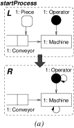
Figure 2: (a) Rule Example. (b) Static Formulation. (c) Dynamic Formulation.

Completion. In order to operate with the matrix representation of graphs of different sizes, an operation called completion adds extra rows and columns with zeros to matrices and vectors and rearranges rows and columns so that the identified edges and nodes of the two graphs match. For example, in Fig. 2, if we need to operate $L^{E}$ and $R^{E}$, completion adds a fourth 0-row and fourth 0-column to $R^{E}$.

Stated in another way, whenever we have to operate graphs $G^{1}$ and $G^{2}$, a morphism $f\colon G^{1}\rightarrow G^{2}$ (i.e. a partial function) has to be defined. Completion rearranges the matrices and vectors of both graphs so that the elements in $Dom(f)$ end up in the same row and column of the matrices. Thus, after the completion we have that $G^{1}\wedge G^{2}\cong Dom(f)$. In the examples, we omit such operation, assuming that matrices are completed when necessary. Later we will operate with the matrices of different productions, thus we have to select the elements (nodes and edges) of each rule that get identified to the same element in the host graph. That is, one has to establish morphisms between the LHS and RHS of the different rules, and completion rearranges the matrices according to the morphisms. Note that there may be different ways to complete two matrices, by chosing different orderings for its rows and columns. This is because a simple digraph can be represented by many adjacency matrices, which differ in the order of rows and columns. In any case, the graphs represented by the matrices are the same.

Nihilation Matrix. In order to consider the elements in the host graph that disable a rule application, we extend the notation for rules with a new graph $N$. Its associated matrix $N^{E}$ specifies the two kinds of forbidden edges: those incident to nodes which are going to be erased and any edge added by the rule (which cannot be added twice, since we are dealing with simple digraphs). Notice however that $N^{E}$ considers only potential dangling edges with source and target in the nodes belonging to $L^{V}$.

Definition 2.7 (Nihilation Matrix)

Given the production $p=(L=(L^{E},L^{V},type^{L});e^{E},r^{E};e^{V},$ $r^{V};type^{r})$, its nihilation matrix $N^{E}$ contains non-zero elements in positions corresponding to newly added edges, and to non-deleted edges adjacent to deleted nodes.

We extend the rule formulation with this nihilation matrix. The concept of rule remains unaltered because we are just making explicit some implicit information. Matrices are derived in the following order: $\left(L,R\right)\mapsto\left(e,r\right)\mapsto N^{E}$. Thus, a rule is statically determined by its LHS and RHS $p=\left(L,R\right)$, from which it is possible to give a dynamic definition $p=\left(L;e,r\right)$, with $e=L\overline{R}$ and $r=R\overline{L}$, to end up with a full specification including its environmental behaviour $p=\left(L,N^{E};e,r\right)$. No extra effort is needed from the grammar designer, because $N^{E}$ can be automatically calculated as the image by rule $p$ of a certain matrix (see proposition 2.9).

Definition 2.8 (Full Dynamic Formulation of Production)

A production $p:L\rightarrow R$ is dynamically represented as $p=(L=(L^{E},L^{V},type^{L});N^{E};e^{E},r^{E};$ $e^{V},r^{V};type^{r})$, where $N^{E}$ is the nihilation matrix, $e^{E}$ and $e^{V}$ are the deletion Boolean matrix and vector, and $r^{E}$ and $r^{V}$ are the addition Boolean matrix and vector.

Next proposition shows how to calculate the nihilation matrix using the production $p$, by applying it to a certain matrix.

Proposition 2.9 (Nihilation matrix)

The nihilation matrix $N^{E}$ of a given production $p$ is calculated as $N^{E}=p\left(\overline{D}\right)$ with $D=\overline{e^{V}}\otimes\overline{e^{V}}^{t}$.

Proof. Matrix $\overline{D}$ specifies potential dangling edges incident to nodes in $p$’s LHS:

$$\overline{D}=d^{i}_{\!j}=\left\{\begin{array}[]{ll}1&\qquad if\;(e^{V})^{i}=1\;or\;(e^{V})^{j}=1.\\ 0&\qquad otherwise.\end{array}\right.$$ (1)

Note that $D=\overline{e^{V}}\otimes\overline{e^{V}}^{t}$. Every incident edge to a node that is deleted becomes dangling, except those explicitly deleted by the production. In addition, edges added by the rule cannot be present in the host graph, $N^{E}=r^{E}\vee\overline{e^{E}}\left(\overline{D}\right)=p\left(\overline{D}\right)$. $\blacksquare$

Example. The nihilation matrix $N^{E}$ for the example rule of Fig. 2 is calculated as follows:

$$\overline{\overline{e^{V}}\otimes\overline{\left(e^{V}\right)}^{\,t}}=\overline{\left[\begin{array}[]{c}1\\ 1\\ 1\\ 0\\ \end{array}\right]\otimes\left[\begin{array}[]{c}1\\ 1\\ 1\\ 0\\ \end{array}\right]^{t}}=\left[\begin{array}[]{cccc}0&0&0&1\\ 0&0&0&1\\ 0&0&0&1\\ 1&1&1&1\\ \end{array}\right]$$

The nihilation matrix is then given by :

$$N^{E}=r\vee\overline{e}\overline{D}=\left[\begin{array}[]{cccc}0&0&0&0\\ 0&1&0&0\\ 0&0&1&0\\ 0&0&0&0\\ \end{array}\right]\vee\overline{\left[\begin{array}[]{cccc}0&0&0&0\\ 0&0&0&0\\ 0&0&0&0\\ 1&0&0&0\\ \end{array}\right]}\left[\begin{array}[]{cccc}0&0&0&1\\ 0&0&0&1\\ 0&0&0&1\\ 1&1&1&1\\ \end{array}\right]=\left[\begin{array}[]{cccc}0&0&0&1\\ 0&1&0&1\\ 0&0&1&1\\ 0&1&1&1\\ \end{array}\right]$$

The matrix indicates any dangling edge from the deleted piece (the edge to the conveyor is not signaled as it is explicitly deleted), as well as self-loops in the machine and in the operator.

Figure 3: $N^{E}$ Graph for startProcess.

Matrix $N^{E}$ can be extended to a simple digraph by taking the nodes in the LHS: $N=(N^{E},L^{V})$. Note that it defines a simple digraph, as one basically needs to add the source and target nodes of the edges in $N^{E}$, which are a subset of the nodes in $L^{V}$, because for the calculation of $N^{E}$ we have used the edges stemming from the nodes in $L^{V}$. Fig. 3 shows the graph representation for the nihilation matrix of previous example. The nihilation matrix should not be confused with the notion of Negative Application Condition (NAC) [8], which is an additional graph specified by the designer (i.e. not derived from the rule) containing extra negative conditions. $\blacksquare$

The evolution of the rule’s LHS (i.e. how it is transformed into the RHS) is given by the production itself ($R=p(L)=r\vee\overline{e}\,L$). It is interesting to analyse the behaviour of the nihilation matrix, which is given by the next proposition.

Proposition 2.10 (Evolution of the Nihilation Matrix)

Let $p:L\rightarrow R$ be a compatible production with nihilation matrix $N^{E}$. Then, the elements that must not appear once the production is applied are given by $p^{-1}\left(N^{E}\right)$, where $p^{-1}$ is the inverse of $p$ (the production that adds what $p$ deletes and vice versa, obtained by swapping $e$ and $r$).

Proof. The elements that should not appear in the RHS are potential dangling edges and those deleted by the production: $e\vee\overline{D}$. This coincides with $p^{-1}(N^{E})$ as shown by the following set of identities:

$$p^{-1}\left(N^{E}\right)=e\vee\overline{r}\,N^{E}=e\vee\overline{r}\left(r\vee\overline{e}\,\overline{D}\right)=e\vee\overline{e}\,\overline{r}\,\overline{D}=e\vee\overline{r}\,\overline{D}=e\vee\overline{D}.$$ (2)

In the last equality of (2) compatibility has been used, $\overline{r}\,\overline{D}=\overline{D}$. $\blacksquare$

Remark. Though strange at a first glance, a dual behaviour of the negative part of a production with respect to the positive part should be expected. The fact that $N^{E}$ uses $p^{-1}$ rather than $p$ for its evolution is quite natural. When a production $p$ erases one element, it asks its LHS to include it, so it demands its presence. The opposite happens when $p$ adds some element. For $N^{E}$ things happen in the opposite direction. If the production asks for the addition of some element, then the size of $N^{E}$ (its number of edges) is increased while if some element is deleted, $N^{E}$ shrinks.

Example. Fig. 4 shows the calculation of $startProcess^{-1}(N^{E})$ using the graph representation of the matrices in equation 2. $\blacksquare$

Figure 4: Evolution of Nihilation Matrix.

Next definition introduces a functional notation for rules (already used in [22]), inspired by the Dirac or bra-ket notation [2]. This notation will be useful for reasoning and proving the propositions in Section 5.

Definition 2.11 (Functional Formulation of Production)

A production $p:L\rightarrow R$ can be depicted as $R=p(L)=\left\langle L,p\right\rangle$, splitting the static part (initial state, $L$) from the dynamics (element addition and deletion, $p$).

Using such formulation, the ket operators (i.e. those to the right side of the bra-ket) can be moved to the bra (i.e. left hand side) by using their adjoints (which are usually decorated with an asterisk). We make use of this notation in Section 5.

Match and Derivations. Matching is the operation of identifying the LHS of a rule inside a host graph (we consider only injective matches). Given rule $p:L\rightarrow R$ and a simple digraph $G$, any total injective morphism $m:L\rightarrow G$ is a match for $p$ in $G$, thus it is one of the ways of completing $L$ in $G$. The following definition considers not only the elements that should be present in the host graph $G$ (those in $L$) but also those that should not (those in the nihilation matrix, $N^{E}$).

Definition 2.12 (Direct Derivation)

Given rule $p:L\rightarrow R$ and graph $G=(G^{E},G^{V})$ as in Fig. 5(a), $d=\left(p,m\right)$ – with $m=\left(m_{L},m^{E}_{N}\right)$ – is called a direct derivation with result $H=p^{*}\left(G\right)$ if the following conditions are satisfied:

1. There exist total injective morphisms $m_{L}:L\rightarrow G$ and $m^{E}_{N}:N^{E}\rightarrow\overline{G^{E}}$.

2. $m_{L}(n)=m^{E}_{N}(n)$, $\forall n\in L^{V}$.

3. The match $m_{L}$ induces a completion of $L$ in $G$. Matrices $e$ and $r$ are then completed in the same way to yield $e^{*}$ and $r^{*}$. The output graph is calculated as $H=p^{*}(G)=r^{*}\vee\overline{e^{*}}G$.

Figure 5: (a) Direct Derivation. (b) Example.

Remark. Item 2 is needed to ensure that $L$ and $N^{E}$ are matched to the same nodes in $G$.

Example. Fig. 5(b) shows the application of rule startProcess to graph $G$. We have also depicted the inclusion of $N^{E}$ in $\overline{G^{E}}$ (bidirectional arrows have been used for simplification). $\overline{G^{E}}$ is the complement (negation) of matrix $G^{E}$. $\blacksquare$

It is useful to consider the structure defined by the negation of the host graph, $\overline{G}=(\overline{G^{E}},\overline{G^{V}})$. It is made up of the graph $\overline{G^{E}}$ and the vector of nodes $\overline{G^{V}}$. Note that the negation of a graph is not a graph because in general compatibility fails, that is why the term “structure” is used.

The complement of a graph coincides with the negation of the adjacency matrix, but while negation is just the logical operation, taking the complement means that a completion operation has been performed before. Hence, taking the complement of a matrix $G^{E}$ is the negation with respect to some appropriate completion of $G$. That is, the complement of graph $G$ with respect to graph $A$, through a morphism $f\colon A\rightarrow G$ is a two-step operation: (i) complete $G$ and $A$ according to $f$, yielding $G^{\prime}$ and $A^{\prime}$; (ii) negate $G^{\prime}$. As long as no confusion arises negation and complements will not be syntactically distinguished.

Figure 6: Finding Complement and negation of a Graph.

Examples. Suppose we have two graphs $A$ and $G$ as those depicted in Fig. 6 and that we want to check that $A$ is not in $G$. Note that $A$ is not contained in $\overline{G}$ (an operator node does not even appear), but it does appear in the negation of the completion of $G$ with respect to $A$ (graph $\overline{G}_{A}$ in the same figure).

In the context of Fig. 5(b), we see that there is an inclusion $startProcess^{-1}(N^{E})\rightarrow\overline{H}$ (i.e. the forbidden elements after applying production $startProcess$ are not in $H$). This is so because we complete $H$ with an additional piece (which was deleted from $G$). Note also that in Definition 2.12, we have to complete $L$ and $G$ (step 3). As an occurrence of $L$ has to be found in $G$, all nodes of $L$ have to be present in $G$ and thus $G$ is big enough to be able to find an inclusion $N^{E}\rightarrow\overline{G^{E}}$. $\blacksquare$

When applying a rule, dangling edges can occur. This is possible because the nihilation matrix only considers dangling edges to nodes appearing in the rule’s LHS. However, a dangling edge can occur between a node deleted by the rule and a node not considered by the rule’s LHS. In MGG, we propose an SPO-like behaviour [21], where the dangling edges are deleted. Thus, if rule $p$ produces dangling edges (a fact that is partially signaled by $m_{N}$) it is enlarged to explicitly consider the dangling edges in the LHS. This is equivalent to adding a pre-production (called $\varepsilon-$production) to be applied before the original rule [22]. Thus, rule $p$ is transformed into sequence $p;p_{\varepsilon}$ (applied from right to left), where $p_{\varepsilon}$ deletes the dangling edges and $p$ is applied as it is. In order to ensure that both productions are applied to the same elements (matches are non-deterministic), we defined a marking operator $T_{\mu}$ which modifies the rules, so that the resulting rule $T_{\mu}$($p_{\varepsilon}$), in addition, adds a special node connected to the elements to be marked, and $T_{\mu}(p)$ in addition considers the special node in the LHS and then deletes it. This is a technique to control rule application by passing the match from one rule to the next.

Analysis Techniques. In [21, 22, 23, 25] we developed some analysis techniques for MGGs, we briefly give an intuition to those that will be used in Section 5.2.

One of the goals of our previous work was to analyse rule sequences independently of a host graph. We represent a rule sequence as $s_{n}=p_{n};...;p_{1}$, where application is from right to left (i.e. $p_{1}$ is applied first). For its analysis, we complete the sequence, by identifying the nodes across rules which are assumed to be mapped to the same node in the host graph.

Once the sequence is completed, our notion of sequence coherence [21] [26] [25] permits knowing if, for the given identification, the sequence is potentially applicable (i.e. if no rule disturbs the application of those following it). The formula for coherence results in a matrix and a vector (which can be interpreted as a graph) with the problematic elements. If the sequence is coherent, both should be zero, if not, they contain the problematic elements. A coherent sequence is compatible if its application produces a simple digraph. That is, no dangling edges are produced in intermediate steps.

Given a completed sequence, the minimal initial digraph (MID) is the smallest graph that permits applying such sequence. Conversely, the negative initial digraph (NID) contains all elements that should not be present in the host graph for the sequence to be applicable. In this way, the NID is a graph that should be found in $\overline{G}$ for the sequence to be applicable (i.e. none of its edges can be found in $G$). If the sequence is not completed (i.e. no overlapping of rules is decided), we can also give the set of all graphs able to fire such sequence or spoil its application. We call them initial digraph set and negative digraph set respectively. See section 6 in [26] or sections 4.4 and 5.3 in [25].

Other concepts we developed aim at checking sequential independence (i.e. same result) between a sequence and a permutation of it. G-Congruence detects if two sequences (one permutation of the other) have the same MID and NID. It returns two matrices and two vectors, representing two graphs, which are the differences between the MIDs and NIDs of each sequence respectively. Thus if zero, the sequences have the same MID and NID. Two coherent and compatible completed sequences that are G-congruent are sequential independent. See section 7 in [26] or section 6.1 in [25].

3 Graph Constraints and Application Conditions

In this section, we present our concepts of graph constraints (GCs) and application conditions (ACs). A GC is defined as a diagram plus a MSOL formula. The diagram is made of a set of graphs and morphisms (partial injective functions) which specify the relationship between elements of the graphs. The formula specifies the conditions to be satisfied in order to make a host graph $G$ satisfy the GC (i.e. we check whether $G$ is a model for the diagram and the formula). The domain of discourse of the formulae are simple digraphs, and the diagram is a means to represent the interpretation function I.

GC formulae are made of expressions about graph inclusions. For this purpose, we introduce the following two predicates:

$$P(X_{1},X_{2})=\forall m[F(m,X_{1})\Rightarrow F(m,X_{2})]$$ (3)

$$Q(X_{1},X_{2})=\exists e[F(e,X_{1})\wedge F(e,X_{2})]$$ (4)

where predicate $F(m,X)$ states that element $m$ (a node or an edge) is in graph $X$. In this way, predicate $P(X_{1},X_{2})$ means that graph $X_{1}$ is included in $X_{2}$. Note that $m$ ranges over all nodes and edges (edges are defined by their initial and final node) of $X_{1}$, thus ensuring the containment of $X_{1}$ in $X_{2}$ (i.e. preserving the graph structure). Predicate $Q(X_{1},X_{2})$ asserts that there is a partial morphism between $X_{1}$ and $X_{2}$, which is defined on at least one edge. That is, $X_{1}$ and $X_{2}$ share an edge. In this case, $e$ ranges over all edges.

Predicates decorated with superindices $E$ or $V$ refer to Edges or Vertices. Thus, $P^{V}(X_{1},X_{2})$ says that every vertex in graph $X_{1}$ should also be present in $X_{2}$. Actually $P(X_{1},X_{2})$ is in fact a shortcut for stating that all vertices in $X_{1}$ should be found in $X_{2}$ ($P^{V}(X_{1},X_{2})$), all edges in $X_{1}$ should be found in $X_{2}$ ($P^{E}(X_{1},X_{2})$) and in addition the set of nodes found should correspond to the source and target nodes of the edges.

Predicate $P(X_{1},X_{2})$ asks for an inclusion morphism $d_{12}:X_{1}\hookrightarrow X_{2}$. The diagram of the constraint may already include such morphism $d_{12}$ (i.e. the diagram can be seen as a set of restrictions imposed on the interpretation function I) and we can either permit extensions of $d_{12}$ (i.e. the model – host graph – may relate more elements of $X_{1}$ and $X_{2}$) or keep it as defined in the diagram. In this latter case, the host graph should identify exactly the specified elements in $d_{12}$ and keep different the elements not related by $d_{12}$. This is represented using predicate $P_{U}$, which can be expressed using $P^{E}$:

$$P^{E}_{U}(X_{1},X_{2})=\forall a[\neg(F(a,D)+F(a,coD))]=P^{E}(D,coD)\wedge P^{E}(D^{C},coD^{C})$$ (5)

where $D=Dom(d_{12})$, $coD=coDom(d_{12})$, ^C stands for the complement (i.e. $D^{C}$ is the complement of $Dom(d_{12})$ w.r.t $X_{1}$) and $+$ is the xor operation. A similar reasoning applies to nodes.

The notation (syntax) will be simplified by making the host graph $G$ the default second argument for predicates $P$ and $Q$. Besides, it will be assumed that by default total morphisms are demanded: unless otherwise stated predicate $P$ is assumed.

Figure 7: Diagram Example.

Example. Before starting with formal definitions, we give an intuition of GCs. The following GC is satisfied if for every $A_{0}$ in $G$ it is possible to find a related $A_{1}$ in $G$: $\forall A_{0}\exists A_{1}\left[A_{0}\Rightarrow A_{1}\right]$, equivalent by definition to $\forall A_{0}\exists A_{1}\left[P\!\!\left(A_{0},G\right)\Rightarrow P\!\!\left(A_{1},G\right)\right]$. Nodes and edges in $A_{0}$ and $A_{1}$ are related through the diagram shown in Fig. 7, which relates elements with the same number and type. As a notational convenience, to enhance readability, each graph in the diagram has been marked with the quantifier given in the formula. If a total match is sought, no additional inscription is presented, but if a partial match is demanded the graph is additionally marked with a $Q$. Similarly, if a total match is forbidden by the formula, the graph is marked with $\overline{P}$. This convention will be used in most examples throughout the paper. The GC in Fig. 7 expresses that each machine should have an output conveyor.$\blacksquare$

Note the identity $\overline{P}(A,G)=Q(A,\overline{G})$, which we use throughout the paper. We take the convention that negations in abbreviations apply to the predicate (e.g., $\exists A\left[\overline{A}\right]\equiv\exists A\left[\overline{P}\left(A,G\right)\right]$) and not the negation of the graph’s adjacency matrix.

A bit more formally, the syntax of well-formed formulas is inductively defined as in monadic second-order logic, which is first-order logic plus variables for subsets of the domain of discourse. Across this paper, formulas will normally have one variable term $G$ which represents the host graph. Usually, the rest of the terms will be given (they will be constant terms). Predicates will consist of $P$ and $Q$ and combinations of them through negation and binary connectives. Next definition formally presents the notion of diagram.

Definition 3.1 (Diagram)

A diagram $\mathfrak{d}$ is a set of simple digraphs $\{A_{i}\}_{i\in I}$ and a set of partial injective morphisms $\{d_{k}\}_{k\in K}$ with $d_{k}:A_{i}\rightarrow A_{j}$. Diagram $\mathfrak{d}$ is well defined if every cycle of morphisms commute.

The formulae in the constraints use variables in the set $\{A_{i}\}_{i\in I}$, and predicates $P$ and $Q$. Formulae are restricted to have no free variables except for the default second argument of predicates $P$ and $Q$, which is the host graph $G$ in which we evaluate the GC. Next definition presents the notion of GC.

Definition 3.2 (Graph Constraint)

$GC=(\mathfrak{d}=(\{A_{i}\}_{i\in I},\{d_{j}\}_{j\in J}),\mathfrak{f})$ is a graph constraint, where $\mathfrak{d}$ is a well defined diagram and $\mathfrak{f}$ a sentence with variables in $\{A_{i}\}_{i\in I}$. A constraint is called basic if $|I|=2$ (with one bound variable and one free variable) and $J=\emptyset$.

In general, there will be an outstanding variable among the $A_{i}$ representing the host graph, being the only free variable in $\mathfrak{f}$. In previous paragraphs it has been denoted by $G$, the default second argument for predicates $P$ and $Q$. We sometimes speak of a “GC defined over G”. A basic GC will be one made of just one graph and no morphisms in the diagram (recall that the host graph is not represented by default in the diagram nor included in the formulas).

Next, we define an AC as a GC where exactly one of the graphs in the diagram is the rule’s LHS (existentially quantified over the host graph) and another one is the graph induced by the nihilation matrix (existentially quantified over the negation of the host graph).

Definition 3.3 (Application Condition)

Given rule $p:L\rightarrow R$ with nihilation matrix $N^{E}$, an AC (over the free variable $G$) is a GC satisfying:

1. $\exists!i,j$ such that $A_{i}=L$ and $A_{j}=N^{E}$.

2. $\exists!k$ such that $A_{k}=G$ is the only free variable.

3. $\mathfrak{f}$ must demand the existence of $L$ in $G$ and the existence of $N^{E}$ in $\overline{G^{E}}$.

The simple graph $G$ can be thought of as a host graph to which some grammar rules are to be applied. For simplicity, we usually do not explicitly show the condition 3 in the formulae of ACs, nor the nihilation matrix $N^{E}$ in the diagram. However, if omitted, both $L$ and $N^{E}$ are existentially quantified before any other graph of the AC. Thus, an AC has the form $\exists L\nexists N^{E}...[L\wedge P(N^{E},\overline{G})\wedge...]$. Note the similarities between Def. 3.3 and that of derivation in Def. 2.12.

Actually, we can interpret the rule’s LHS and its nihilation matrix as the minimal AC a rule can have. Hence, any well defined production has a natural associated AC. Note also that, in addition to the AC diagram, the structure of the rule itself imposes a relation between $L$ and $N^{E}$ (and between $L$ and $R$). For technical reasons, related to converting pre- into post-conditions and viceversa, we assume that morphisms in the diagram do not have codomain $L$ or $N^{E}$. This is easily solved as we may always use their inverses due to $d_{i}$’s injectiveness.

Semantics of Quantification. In GCs or ACs, graphs are quantified either existentially or universally. We now give the intuition of the semantics of such quantification applied to basic formulae. Thus, we consider the four basic cases: (i) $\exists A[A]$, (ii) $\forall A[A]$, (iii) $\nexists A[A]$, (iv) $/\!\!\forall A[A]$.

Case (i) states that $G$ should include graph $A$. For example, in Fig. 8, the GC $\exists opMachine$ $[opMachine]$ demands an occurrence of $opMachine$ in $G$ (which exists).

Figure 8: Quantification Example.

Case (ii) demands that, for all potential occurrences of $A$ in $G$, the shape of graph $A$ is actually found. The term potential occurrences means all distinct maximal partial matches (which are total on nodes) of $A$ in $G$. A non-empty partial match in $G$ is maximal, if it is not strictly included in another partial or total match. For example, consider the GC $\forall opMachine[opMachine]$ in the context of Fig. 8. There are two possible instantiations of $opMachine$ (as there are two machines and one operator), and these are the two input elements to the formula. As only one of them satisfies $P(opMachine,G)$ – the expanded form of $[opMachine]$ – the GC is not satisfied by $G$.

Case (iii) demands that, for all potential occurrences of $A$, none of them should have the shape of $A$. The term potential occurrence has the same meaning as in case (ii). In Fig. 8, there are two potential instantiations of the GC $\nexists opMachine[opMachine]$. As one of them actually satisfies $P(opMachine,G)$, the formula is not satisfied by $G$.

Finally, case (iv) is equivalent to $\exists A[\overline{A}]$, where by definition $\overline{A}\equiv\overline{P}(A,G)$. This GC states that for all possible instantiations of $A$, one of them must not have the shape of $A$. This means that a non-empty partial morphism $A\rightarrow\overline{G}$ should be found. The GC $\exists opMachine[\overline{opMachine}]$ in Fig. 8 is satisfied by $G$ because, again, there are two possible instantiations, and one of them actually does not have an edge between the operator and the machine.

Next definition formalizes the previous intuition, where we use the following notation:

• $par^{max}(A,G)=\{f\colon A\rightarrow G|f$ is a maximal non-empty partial morphism s.t. $Dom(f)^{V}=A^{V}\}$

• $tot(A,G)=\{f\colon A\rightarrow G|f$ is a total morphism $\}\subseteq par^{max}(A,G)$

• $iso(A,G)=\{f\colon A\rightarrow G|f$ is an isomorphism $\}\subseteq tot(A,G)$

where $Dom(f)^{V}$ are the nodes of the graph in the domain of $f$. Thus, $par^{max}(A,G)$ denotes the set of all potential occurrences of a given constraint graph $A$ in $G$, where we require all nodes in $A$ be present in the domain of $f$. Note that each $f\in par^{max}$ may be empty in edges.

Definition 3.4 (Basic Constraint Satisfaction)

The host graph $G$ satisfies $\exists A[A]$, written $G\models\exists A[A]$ iff $\exists f\in par^{max}(A,G)\>[f\in tot(A,G)]$.
The host graph $G$ satisfies $\forall A[A]$, writteni $G\models\forall A[A]$ iff $\forall f\in par^{max}(A,G)\>[f\in tot(A,G)]$.

The diagrams associated to the formulas in previous definition have been omitted for simplicity as they consist of a single element: $A$. Recall that by default predicate $P$ is assumed as well as $G$ as second argument, e.g. the first formula in previous definition $\exists A[A]$ is actually $\exists A[P(A,G)]$. Note also that only these two cases are needed, as one has $\nexists A[P(A,G)]\equiv\forall A[\overline{P}(A,G)]$ and $/\!\!\forall A[P(A,G)]\equiv\exists A[\overline{P}(A,G)]$.

Thus, this is a standard interpretation of MSOL formulae, save for the domain of discourse (graphs) and therefore the elements of quantification (maximal non-empty partial morphisms). Taking this fact into account, next, we define when a graph satisfies an arbitrary $GC$. This definition also applies to ACs.

Definition 3.5 (Graph Constraint Satisfaction)

We say that $\mathfrak{d}_{0}=(\{A_{i}\},\{d_{j}\})$ satisfies the graph constraint $GC=(\mathfrak{d}=(\{X_{i}\},$$\{d_{j}\}),\mathfrak{f})$ under the interpretation function $I$, written $(I,\mathfrak{d}_{0})\models\mathfrak{f}$, if $\mathfrak{d}_{0}$ is a model for $\mathfrak{f}$ that satisfies the element relations specified by the diagram $\mathfrak{d}$, and the following interpretation for the predicates in $\mathfrak{f}$:

1. $I\left(P\left(X_{i},X_{j}\right)\right)=m^{T}:X_{i}\rightarrow X_{j}$ total injective morphism.

2. $I\left(Q\left(X_{i},X_{j}\right)\right)=m^{P}:X_{i}\rightarrow X_{j}$ partial injective morphism, non-empty in edges.

where $m^{T}|_{D}=d_{k}=m^{P}|_{D}$ with $d_{k}:X_{i}\rightarrow X_{j}$ and $D=Dom\left(d_{k}\right)$. The interpretation of quantification is as in Def. 3.4 but setting $X_{i}$ and $X_{j}$ instead of $A$ and $G$, respectively.

The notation deserves the following comments:

1. The notation $(I,\mathfrak{d}_{0})\models\mathfrak{f}$ means that the formula $\mathfrak{f}$ is satisfied under interpretation given by $I$, assignments given by morphisms specified in $\mathfrak{d}_{0}$ and substituting the variables in $\mathfrak{f}$ with the graphs in $\mathfrak{d}_{0}$.

2. As commented after Def. 3.2, in many cases the formula $\mathfrak{f}$ will have a single variable (the one representing the host graph $G$) and always the interpretation function will be that given in Def. 3.5. We may thus write $G\models\mathfrak{f}$ which is the notation that appears in Def. 3.4. The notation $G\models GC$ may also be used.

3. Similarly, as an AC is just a GC where $L$, $N^{E}$ and $G$ are present, we may write $G\models AC$. For practical purposes, we are interested in testing whether, given a host graph $G$, a certain match $m_{L}\colon L\rightarrow G$ satisfies the AC. In this case we write $(G,m_{L})\models AC$. In this way, the satisfaction of an AC by a match and a host graph is like the satisfaction of a GC by a graph $G$, where a morphism $m_{L}$ is already specified in the diagram of the GC.

Remark. For technical reasons, we require all graphs in the GC for which a partial morphism is demanded to be found in the host graph to have at least one edge and be connected. That is why $m^{P}$ has to be non-empty in edges.

Figure 9: Satisfaction of Application Condition.

Examples. Fig. 9 shows rule contract, with an AC given by the diagram in the figure (where morphisms identify elements with the same type and number, this convention is followed throughout the paper), together with formula $\exists L\>\nexists bMach\>\forall bOp[L\wedge bMach\wedge bOp]$. The rule creates a new operator, and assigns it to a machine. The rule can be applied if there is a match of the LHS (a machine is found), the machine is not busy ($\nexists bMach[bMach]$), and all operators are busy ($\forall bOp[bOp]$). Graph $G$ to the right satisfies the AC, with the match that identifies the machine in the LHS with the machine in $G$ with the same number.

Using the terminology of ACs in the algebraic approach [8], $\nexists bMach[bMach]$ is a negative application condition (NAC). On the other hand, there is no equivalent to $\forall bOp[bOp]$ in the algebraic approach, but in this case it could be emulated by a diagram made of two graphs stating that if an operator exists then it does not have a self-loop. However, this is not possible in all cases as next example shows.

Figure 10: Example of Application Condition.

Fig. 10 shows rule move, which has an AC with formula: $\exists Cv\>\forall AllC\>\exists out\>\exists next[(AllC\wedge out)\Rightarrow$ $(next\wedge Cv)]$. As previously stated, in this example and the followings, the rule’s LHS and the nihilation matrix are omitted in the AC’s formula. The example AC checks whether all conveyors connected to conveyor 1 in the LHS reach a common target conveyor in one step. We can use “global” information, as graph $Cv$ has to be found in $G$ and then all output conveyors are checked to be connected to it ($Cv$ is existentially quantified in the formula before the universal). Note that we first obtain all possible conveyors ($\forall AllC$). As the identifications of the morphism $L\rightarrow AllC$ have to be preserved, we consider only those potential instances of $AllC$ with $1:Conveyor$ equal to $1:Conveyor$ in $L$. From these, we take those that are connected ($\exists out$), and which therefore have to be connected with the conveyor identified by the LHS. Graph $G$ satisfies the AC, while graph $G^{\prime}$ does not, as the target conveyor connected to $5$ is not the same as the one connected to $2$ and $4$. To the best of our efforts it is not possible to express this condition using the standard ACs in the DPO approach given in [8]. $\blacksquare$

4 Embedding Application Conditions into Rules

In this section, the goal is to embed arbitrary ACs into rules by including the positive and negative coditions in $L$ and $N^{E}$ respectively. It is necessary to check that direct derivations can be the codomain of the interpretation function, that is, intuitively we want to assert whether “MGG + AC = MGG” and “MGG + GC = MGG”.

As stated in previous section, in direct derivations, the matching corresponds to formula $\exists L\exists N^{E}$ $\left[L\wedge P\left(N^{E},\overline{G^{E}}\right)\right]$, but additional ACs may represent much more general properties, due to universal quantifiers and partial morphisms. Normally, plain rules (without ACs) in the different approaches to graph transformation do not care about elements that cannot be present. If so, a match is just $\exists L[L]$. Thus, we seek for a means to translate universal quantifiers and partial morphisms into existential quantifiers and total morphisms.

For this purpose, we introduce two operations on basic diagrams: closure ($\mathfrak{C}$), dealing with universal quantifiers only, and decomposition ($\mathfrak{D}$), for partial morphisms only (i.e. with the $Q$ predicate).

The closure operator converts a universal quantification into a number of existentials, as many as maximal partial matches there are in the host graph (see definition 3.4). Thus, given a host graph $G$, demanding the universal appearance of graph $A$ in $G$ is equivalent to asking for the existence of as many replicas of $A$ as partial matches of $A$ are in $G$.

Definition 4.1 (Closure)

Given $GC=\left(\mathfrak{d},\mathfrak{f}\right)$ with diagram $\mathfrak{d}=\{A\}$, ground formula $\mathfrak{f}=\forall A[A]$ and a host graph $G$, the result of applying $\mathfrak{C}$ to $GC$ is calculated as follows:

$$\mathfrak{d} \longmapsto \mathfrak{d}^{\prime}=\left(\{A^{1},\ldots,A^{n}\},d_{ij}:A^{i}\rightarrow A^{j}\right)$$

$$\mathfrak{f} \longmapsto \mathfrak{f}^{\prime}=\exists A^{1}\ldots\exists A^{n}\left[\bigwedge_{i=1}^{n}A^{i}\bigwedge_{i,j=1,j>i}^{n}P_{U}(A^{i},A^{j})\right]$$ (6)

with $A^{i}\cong A$, $d_{ij}\not\in iso(A^{i},A^{j})$, $\mathfrak{C}\left(GC\right)=GC^{\prime}=\left(\mathfrak{d}^{\prime},\mathfrak{f}^{\prime}\right)$ and $n=|par^{max}(A,G)|$.

Remark. Completion creates a morphism $d_{ij}$ between each different $A^{i}$ and $A^{j}$ (both isomorphic to $A$), but morphisms are not needed in both directions (i.e. $d_{ji}$ is not needed). The condition that morphism $d_{ij}$ must not be an isomorphism means that at least one element of $A^{i}$ and $A^{j}$ has to be identified in different places of $G$. This is accomplished by means of predicate $P_{U}$ (see its definition in equation 5), which ensures that the elements not related by $d_{ij}\colon A^{i}\rightarrow A^{j}$, are not related in $G$.

The interpretation of the closure operator is that demanding the universal appearance of a graph is equivalent to the existence of all of its potential instances (i.e. those elements in $par^{max}$) in the specified digraph ($G$, $\overline{G}$ or some other). Some nodes can be the same for different identifications ($d_{ij}$), so the procedure does not take into account morphisms that identify every single node, $d_{ij}\not\in iso(A^{i},A^{j})$. Therefore, each $A^{i}$ contains the image of a potential match of $A$ in $G$ (there are $n$ possible occurrences of $A$ in $G$) and $d_{ij}$ identifies elements considered equal.

Example. Assume the diagram to the left of Fig. 11, made of just graph $gen$, together with formula $\forall gen[gen]$, and graph $G$, where such GC is to be evaluated. The GC asks $G$ for the existence of all potential connections between each generator and each conveyor. Performing closure we obtain $\mathfrak{C}((gen,\forall gen[gen]))=(\mathfrak{d}_{C},\exists gen_{1}\exists gen_{2}\exists gen_{3}[gen_{1}\wedge gen_{2}\wedge gen_{3}\wedge P_{U}(gen_{1},gen_{2})\wedge P_{U}(gen_{1},gen_{3})\wedge P_{U}(gen_{2},gen_{3})])$, where diagram $\mathfrak{d}_{C}$ is shown to the right of Fig. 11, and each $d_{ij}$ identifies elements with the same number and type. The closure operator makes explicit that three potential occurrences must be found (as $|par^{max}(gen,G)|=3$), thus, taking information from the graph where the GC is evaluated and placing it in the GC itself. $\blacksquare$

Figure 11: (a) GC diagram. (b) Graph where GC is to be evaluated. (c) Closure of GC w.r.t. G.

The idea behind decomposition is to split a graph into its basic components to transform partial morphisms into total morphisms of one of its parts. For this purpose, the decomposition operator $\mathfrak{D}$ splits a digraph $A$ into its edges, generating as many digraphs as edges in $A$. As stated in remark 1 of definition 3.5, all graphs for which the GC asks for a partial morphism are forbidden to have isolated nodes. We are more interested in the behaviour of edges (which to some extent comprises nodes as source and target elements of the edges, except for isolated nodes) than on nodes alone as they define the topology of the graph. This is also the reason why predicate $Q$ was defined to be true in the presence of a partial morphism non-empty in edges. If so desired, in order to consider isolated nodes, it is possible to define two decomposition operators, one for nodes and one for edges, but this is left for future work.

Definition 4.2 (Decomposition)

Given $GC=\left(\mathfrak{d},\mathfrak{f}\right)$ with ground formula $\mathfrak{f}=\exists A[Q(A)]$ and diagram $\mathfrak{d}=\{A\}$, $\mathfrak{D}$ acts on $GC$ – $\mathfrak{D}\left(GC\right)=AC^{\prime}=\left(\mathfrak{d}^{\prime},\mathfrak{f}^{\prime}\right)$ – in the following way:

$$\mathfrak{d} \longmapsto \mathfrak{d}^{\prime}=\left(\{A^{1},\ldots,A^{n}\},d_{ij}:A^{i}\rightarrow A^{j}\right)$$

$$\mathfrak{f} \longmapsto \mathfrak{f}^{\prime}=\exists A^{1}\ldots\exists A^{n}\left[\bigvee_{i=1}^{n}A^{i}\right]$$ (7)

with $n=\#\{edg(A)\}$, the number of edges of $A$, and $Q(A^{i},A)$, where $A^{i}$ contains a single edge of $A$.

Demanding a partial morphism is equivalent to asking for the existence of a total morphism of some of its edges, that is, each $A^{i}$ contains exactly one of the edges of $A$.

Example. Consider $GC=(oneP,\exists oneP[Q(oneP)])$, where graph $oneP$ is shown to the left of Fig. 12. The constraint is satisfied by a host graph $G$ if there is a partial morphism non-empty in edges $m^{P}\colon oneP\rightarrow G$. Thus, we require that either the two conveyors are connected, or there is a piece in one of them. Using decomposition, we obtain $\mathfrak{D}(GC)=(\mathfrak{d}_{D},\exists oneP_{1}\exists oneP_{2}\exists oneP_{3}$ $[oneP_{1}\vee oneP_{2}\vee oneP_{3}])$. Diagram $\mathfrak{d}_{D}$ is shown in Fig. 12(b), together with a graph $G$ satisfying the constraint in Fig. 12(c). Note that this constraint can be expressed more concisely than in other approaches, like the algebraic/categorical one of [8].

Figure 12: (a) GC diagram. (b) Decomposition of the GC. (c) Graph satisfying the GC.

Note how, decomposition is not affected by the host graph to which it is to be evaluated. Also, we do not care whether some graphs in the decomposition are matched in the same place in the host graph (e.g. $oneP_{1}$ and $oneP_{3}$), as the GC just requires one of them to be found. $\blacksquare$

Now we show the main result of this section, which states that it is possible to reduce any formula in an AC (or GC) into another one using existential quantifiers and total morphisms only. This theorem is of interest because derivations as defined in MGGs (the matching part) use only total morphisms and existential quantifiers.

Theorem 4.3 ($\exists-P$ reduction)

Let $GC=\left(\mathfrak{d},\mathfrak{f}\left(P,Q\right)\right)$ with $\mathfrak{f}$ a ground formula, $\mathfrak{f}$ can be transformed into a logically equivalent $\mathfrak{f^{\prime}}=\mathfrak{f}^{\prime}(P)$ with existential quantifiers only.

Proof. Let the depth of a graph for a fixed node $n_{0}$ be the maximum over the shortest path (to avoid cycles) starting in any node different from $n_{0}$ and ending in $n_{0}$. The depth of a graph is the maximum depth for all its nodes. Diagram $\mathfrak{d}$ is a graph where nodes are digraphs $A_{i}$ and edges are morphisms $d_{ij}$. We use $depth\left(GC\right)$ to denote the depth of $\mathfrak{d}$. In order to prove the theorem we apply induction on the depth, checking out every case. There are 16 possibilities for $depth\left(\mathfrak{d}\right)=1$ and a single element $A$, summarized in Table 1.

I(1)	$\exists A[A]$	(5)	$/\!\!\forall A[\overline{A}]$	(9)	$\exists A[\overline{Q}(A)]$	(13)	$/\!\!\forall A[Q(A)]$
I(2)	$\exists A[\overline{A}]$	(6)	$/\!\!\forall A[A]$	(10)	$\exists A[Q(A)]$	(14)	$/\!\!\forall A[\overline{Q}(A)]$
I(3)	$\nexists A[\overline{A}]$	(7)	$\forall A[A]$	(11)	$\nexists A[Q(A)]$	(15)	$\forall A[\overline{Q}(A)]$
I(4)	$\nexists A[A]$	(8)	$\forall A[\overline{A}]$	(12)	$\nexists A[\overline{Q}(A)]$	(16)	$\forall A[Q(A)]$

Table 1: All Possible Diagrams for a Single Element.

Elements in the same row for each pair of columns are related using equalities $\nexists A[A]=\forall A[\overline{A}]$ and $/\!\!\forall A[A]=\exists A[\overline{A}]$, so it is possible to reduce the study to cases (1)–(4) and (9)–(12). Identities $\overline{Q}(A)=P(A,\overline{G})$ and $Q(A)=\overline{P}(A,\overline{G})$ reduce (9)–(12) to formulae (1)–(4):

$$\exists A[\overline{Q}(A)]=\exists A\left[P(A,\overline{G})\right] \exists A[Q(A)]=\exists A\left[\overline{P}(A,\overline{G})\right]$$ ,

$$\nexists A[Q(A)]=\nexists A\left[\overline{P}(A,\overline{G})\right] \nexists A[\overline{Q}(A)]=\nexists A\left[P(A,\overline{G})\right].$$ ,

Thus, it is enough to study the first four cases, but we have to specify if $A$ must be found in $G$ or $\overline{G}$. Finally, all cases in the first column can be reduced to (1):

• (1) is the definition of match.

• (2) can be transformed into total morphisms (case 1) using operator $\mathfrak{D}$: $\exists A\left[\overline{A}\right]=\exists A\left[Q(A,\overline{G})\right]=\exists A^{1}\ldots\exists A^{n}\left[\bigvee_{i=1}^{n}P\left(A^{i},\overline{G}\right)\right]$.

• (3) can be transformed into total morphisms (case 1) using operator $\mathfrak{C}$: $\nexists A\left[\overline{A}\right]=\forall A[A]=\exists A^{1}\ldots\exists A^{n}\left[\bigwedge_{i=1}^{n}A^{i}\right]$. Here for simplicity, the conditions on $P_{U}$ are assumed to be satisfied and thus have not been included.

• (4) combines (2) and (3), where operators $\mathfrak{C}$ and $\mathfrak{D}$ are applied in order $\mathfrak{D}\circ\mathfrak{C}$ (see remark below): $\nexists A[A]=\forall A\left[\overline{A}\right]=\exists A^{11}\ldots\exists A^{mn}\left[\bigwedge_{i=1}^{m}\bigvee_{j=1}^{n}P\left(A^{ij},\overline{G}\right)\right]$.

If there is more than one element at depth 1, this same procedure can be applied mechanically (well-definedness guarantees independence with respect to the order in which elements are selected). Note that if depth is 1, graphs on the diagram are unrelated (otherwise, depth $>$ 1).

Induction Step. When there is a universal quantifier $\forall A$, according to equation 4.1, elements of $A$ are replicated as many times as potential instances of $A$ can be found in the host graph. In order to continue the application procedure, we have to clone the rest of the diagram for each replica of $A$, except those graphs which are existentially quantified before $A$ in the formula. That is, if we have a formula $\exists B\forall A\exists C$, when performing the closure of $A$, we have to replicate $C$ as many times as $A$, but not $B$. Moreover $B$ has to be connected to each replica of $A$, preserving the identifications of the morphism $B\rightarrow A$. More in detail, when closure is applied to $A$, we iterate on all graphs $B_{j}$ in the diagram:

• If $B_{j}$ is existentially quantified after $A$ ($\forall A...\exists B_{j}$) then it is replicated as many times as $A$. Appropriate morphisms are created between each $A^{i}$ and $B^{i}_{j}$ if a morphism $d\colon A\rightarrow B$ existed. The new morphisms identify elements in $A^{i}$ and $B^{i}_{j}$ according to $d$. This permits finding different matches of $B_{j}$ for each $A^{i}$, some of which can be equal.

• If $B_{j}$ is existentially quantified before $A$ ($\exists B_{j}...\forall A$) then it is not replicated, but just connected to each replica of $A$ if necessary. This ensures that a unique $B_{j}$ has to be found for each $A^{i}$. Moreover, the replication of $A$ has to preserve the shape of the original diagram. That is, if there is a morphism $d\colon B\rightarrow A$, then each $d_{i}\colon B\rightarrow A^{i}$ has to preserve the identifications of $d$ (this means that we take only those $A^{i}$ which preserve the structure of the diagram).

• If $B_{j}$ is universally quantified (no matter if it is quantified before or after $A$), again it is replicated as many times as $A$. Afterwards, $B_{j}$ will itself need to be replicated due to its universality. The order in which these replications are performed is not relevant as $\forall A\forall B_{j}=\forall B_{j}\forall A$.

$\blacksquare$

Remark. Operators $\mathfrak{C}$ and $\mathfrak{D}$ commute, i.e. $\mathfrak{C}\circ\mathfrak{D}=\mathfrak{D}\circ\mathfrak{C}$. In the equation of item 4, the application order does not matter. Composition $\mathfrak{D}\circ\mathfrak{C}$ is a direct translation of $\forall A[\overline{A}]$ , which first considers all appearances of nodes in $A$ and then splits these occurrences into separate digraphs. This is the same as considering every pair of connected nodes in $A$ by one edge and take their closure, i.e, $\mathfrak{C}\circ\mathfrak{D}$.

Example. Fig. 13 shows rule endProc and the diagram of its AC, which has formula: $\exists op\>\forall mac$ $\exists work\>\exists conn[(mac\wedge conn)\Rightarrow(op\wedge work)]$. The AC allows for the application of the rule if all machines connected (as output) to the conveyor in $L$ are operated by the same operator. This is so as the AC considers all machines connected to the LHS conveyor by $\forall mac...\exists conn[mac\wedge conn]$. For these machines, it should be the case that a unique operator ($\exists op$ is placed at the beginning of the formula) is connected to them ($\exists work$).

The bottom of the figure shows the resulting diagram after applying the previous theorem, using graph $G$ to the upper right of the figure. At depth 2, graph $mac$ is replicated three times, as it is universally quantified and there are three machines. Then, the rest of the diagram is replicated, except the graphs quantified before $mac$ ($L$ and $op$). The resulting formula of the AC is $\exists op\>\exists_{i=1}^{3}mac_{i}\>\exists_{i=1}^{3}work_{i}\>\exists_{i=1}^{3}conn_{i}$ $[\bigwedge_{i=1}^{3}((mac_{i}\wedge conn_{i})\Rightarrow(op\wedge work_{i}))]$, where we have omitted the $P_{U}$ predicate (asking that actually three machines have to be found in $G$), and used the abbreviation $\exists_{i=1}^{3}A_{i}\equiv\exists A_{1}\>\exists A_{2}\>\exists A_{3}$. Note that graph $G$ satisfies the AC (using the only match of $L$ in $G$) as machine 1 is not operated by the same operator as machines 2 and 3, however conveyor 1 is not connected to machine 1 as output (thus the left part of the implication is false). $\blacksquare$

Figure 13: Example of Closure of AC with $depth>1$

As an AC is a particular case of graph constraint, we can conclude that it is not necessary to extend the notion of direct derivation in order to consider ACs.

Corollary 4.4

Any application condition $AC=\left(\mathfrak{d},\mathfrak{f}=\mathfrak{f}\left(P,Q\right)\right)$ with $\mathfrak{f}$ a ground formula can be embedded into its corresponding direct derivation.

Now we are able to obtain ACs with existentials and total morphisms only. The next section shows how to translate rules with such ACs into sets of rule sequences.

One of the strengths of MGG compared to other graph transformation approaches is the possibility to analyse grammars independently (to some extent) of the actual host graph. However, the universal quantifier appears to be an insurmountable obstacle: the host graph seems indispensable to know how many instances there are. We will see in section 5.1 that this is not the case.

5 Transforming Application Conditions into Sequences

In this section we transform arbitrary ACs into sequences of plain rules, such that if the original rule with ACs is applicable the sequence is applicable and viceversa. This is very useful, as we may use our analysis techniques for plain rules in order to analyse rules with ACs. Next, we present some properties of ACs which, once the AC is translated into a sequence, can be analysed using the developed theory for sequences.

Definition 5.1 (Coherence, Compatibility, Consistency)

Let $AC=\left(\mathfrak{d},\mathfrak{f}\right)$ be an AC on rule $p:L\rightarrow R$. We say that AC is:

• coherent if it is not a contradiction (i.e. false in all scenarios).

• compatible if, together with the rule’s actions, produces a simple digraph.

• consistent if $\exists G$ host graph such that $G\models AC$ to which the production is applicable.

Coherence of ACs studies whether there are contradictions in it preventing its application in any scenario. Typically, coherence is not satisfied if the condition simultaneously asks for the existence and non-existence of some element. Compatibility of ACs checks whether there are conflicts between the AC and the rule’s actions. Here we have to check for example that if a graph of the $AC$ demands the existence of some edge, then it can not be incident to a node that is deleted by production $p$. Consistency is a kind of well-formedness of the AC when a production is taken into account. Next, we show some examples of non-compatible and non-coherent ACs.

Figure 14: Non-Compatible Application Condition

Examples. Non-compatibility can be avoided at times just rephrasing the AC and the rule. Consider the example to the left of Fig. 14. The rule models the breakdown of a machine by deleting it. The AC states that the machine can be broken if it is being operated. The AC has associated diagram $\mathfrak{d}=\{Operated\}$ and formula $\mathfrak{f}=\exists Operated[Operated]$. As the production deletes the machine and the AC asks for the existence of an edge connecting the operator with the machine, it is for sure that if the rule is applied we will obtain at least one dangling edge.

Figure 15: Non-Coherent AC.

The key point is that the AC asks for the existence of the edge but the production demands its non-existence as it is included in the nihilation matrix $N$. In this case, the rule $break^{\prime}$ depicted to the right of the same figure is equivalent to $p$ but with no potential compatibility issues.

Notice that coherence is fulfilled in the example to the left of Fig. 14 (the AC alone does not encode any contradiction) but not consistency as no host graph can satisfy it.

An example of non-coherent application condition can be found in Fig. 15. The AC has associated formula $\mathfrak{f}=\forall busy\exists work[busy\wedge$ $P(work,\overline{G})]$. There is no problem with the edge deleted by the rule, but with the self-loop of the operator. Note that due to $busy$, it must appear in any potential host graph but $work$ says that it should not be present. $\blacksquare$

We will provide a means to study such properties by converting the AC into a sequence of plain rules and studying the sequence, by applying the analysis techniques already developed in MGG. We will prove that an AC is coherent if its associated sequence is coherent and similarly for compatibility. Also, we will see that an AC is consistent if its associated sequence is applicable in some host graph. As this requires sequences to be both coherent and compatible, and AC is consistent if it is both coherent and compatible [26] [25].

5.1 From ACs to Sequences: The Transformation Procedure

In order to transform a rule with ACs into sequences of plain rules, operators $\mathfrak{C}$ and $\mathfrak{D}$ are expressed with the bra-ket functional notation introduced in definition 2.11. Operators $\mathfrak{C}$ and $\mathfrak{D}$ will be formally represented as $\widecheck{T}_{\!A}$ and $\widehat{T}_{\!A}$, respectively, and we analyse how they act on productions and grammars. We shall follow a case by case study of the demonstration of theorem 4.3 to structure this section. The first case in the proof of theorem 4.3 is the simplest one: a graph $A$ has to be found in $G$.

Lemma 5.2 (Match)

Let $p:L\rightarrow R$ be a rule with $AC=((A,d:L\rightarrow A),\exists A[A])$, $p$ is applicable to graph $G$ iff sequence $p;id_{A}$ is applicable to $G$, where $id_{A}$ is a production with LHS and RHS equal to $A$.

Proof. The AC states that an additional graph $A$ has to be found in the host graph, related to $L$ according to the identifications in $d$. Therefore we can do the or of $A$ and $L$ (according to the identifications specified by $d$), and write the resulting rule using the functional notation of definition 2.11, obtaining $\left\langle L\vee A,p\right\rangle$. Thus applying the rule to its LHS, we obtain $p(L\vee A)=R\vee A$.

Note however that such rule is the composition of the original rule $p$, and rule $id_{A}\colon A\rightarrow A$. Thus, we can write $\left\langle L\vee A,p\right\rangle=\left\langle L,id_{\!A}\circ p\right\rangle=p\circ id_{\!A}$, which proves also that $id^{*}_{\!A}\!\left(L\right)=L\vee A$, the adjoint operator of $id_{\!A}$. The symbol “$\circ$” denotes rule composition according to the identification across rules specified by $d$ (see [21]). Thus, if the $AC$ asks for the existence of a graph, it is possible to enlarge the rule $p\mapsto p\circ id_{\!A}$. The marking operator $T_{\mu}$ permits using concatenation instead of composition $\left\langle L\vee A,p\right\rangle=p;id_{\!A}$. $\blacksquare$

Example. The AC of rule $moveOperator$ in Fig. 16 (a) has associated formula $\exists Ready[Ready]$ (i.e. the operator may move to a machine with an incoming piece). Using previous construction, we obtain that the rule is equivalent to sequence $moveOperator^{\flat};id_{Ready}$, where $moveOperator^{\flat}$ is the original rule without the AC. Rule $id_{Ready}$ is shown in Fig. 16 (b). Alternatively, we could use composition to obtain $moveOperator^{\flat}\circ id_{Ready}$ as shown in Fig. 16 (c). $\blacksquare$

Figure 16: Transforming $\exists Ready[Ready]$ into a Sequence.

The second case in the proof of theorem 4.3 states that some edges of $A$ cannot be found in $G$ for some identification of nodes in $G$, i.e. $/\!\!\forall A\left[A\right]=\exists A\left[\overline{A}\right]$. This corresponds to operator $\widehat{T}_{\!A}$ (decomposition), defined by $\widehat{T}_{\!A}\left(p\right)=\left\{p_{1},\ldots,p_{n}\right\}$. For this purpose, we introduce a kind of conjugate (for edges) of production $id_{A}$, written $\overline{id}_{A}$. The left of Fig. 17 shows $id_{A}$, which preserves (uses but does not delete) all elements of $A$. This is equivalent to demand their existence. In the center we have its conjugate, $\overline{id}_{A}$, which asks for the existence of $A$ in the complement of $G$.

Figure 17: Identity $id_{A}$ (left), Conjugate $\overline{id}_{A}$ for Edges (center), $\overline{id}_{A}$ as Sequence for Edges (right).

Rule $\overline{id}_{A}$ for edges can be defined on the basis of already known concepts (i.e. having a “normal” nihilation matrix, according to proposition 2.9). Since $N=r\vee\overline{e}\,\overline{D}$, in order to obtain a rule applicable iff $A^{E}$ is in $\overline{G^{E}}$, the only chance is to act on the elements that some rule adds. Let $p_{e};p_{r}$ be a sequence such that $p_{r}$ adds the edges whose presence is to be avoided and $p_{e}$ deletes them. The overall effect is the identity (no effect) but the sequence can be applied iff the edges of $A$ are in $\overline{G^{E}}$ (see the right of Fig. 17). A similar construction does not work for nodes because if a node is already present in the host graph a new one can always be added (adding and deleting a node does not guarantee that the node is not present in the host graph). Thus, we restrict to diagrams made of graphs without isolated nodes. The way to proceed is to care only about nodes that are present in the host graph as the others together with their edges will be present in the completion of the complement of $G$. This is $A^{V}_{R}$, where $R$ stands for restriction.

Next lemma uses the previous conjugate rule to convert the ACs in the second case of theorem 4.3 into a set of rule sequences.

Lemma 5.3 (Decomposition)

Let $p:L\rightarrow R$ be a rule with $AC=((A,d:L\rightarrow A),/\!\!\forall A\left[A\right])$, $p$ is applicable to graph $G$ iff some sequence in the set $\{s_{i}=p;\overline{id}_{A^{i}}\}$ is applicable to graph $G$, with $\overline{id}_{A^{i}}$ the edge conjugate rule obtained from each graph $A^{i}$ in the decomposition of $A$.

Proof. Let $n$ be the number of edges of $A$, and $A^{i}$ a graph consisting of one edge of $A$ (together with its source and target nodes). Applying decomposition, the formula is transformed into: $\mathfrak{f}=\exists A[\overline{A}]\longmapsto\mathfrak{f}^{\prime}=\exists A^{1}\ldots\exists A^{n}\left[\bigvee^{n}_{i=1}P\left(A^{i},\overline{G}\right)\right]$. That is, the AC indicates that more edges must not appear in order to apply the production. We build the set $\{p_{i}\}_{i\in\{1..n\}}$, where each production $p_{i}$ is equal to $p$, but its nihilation matrix is enlarged with $N_{i}=N\vee A^{i}$. Thus, some production in this set will be applicable iff some edge of $A$ is found in $\overline{G}$ (i.e. iff $\overline{P}(A,G)$ holds) and $p$ is applicable. But note that $p_{i}=p\circ\overline{id}_{\!A^{i}}$, where $\overline{id}_{\!A^{i}}$ is depicted in the center of Fig. 17.

If composition is chosen instead of concatenation, the grammar is modified by removing rule $p$ and adding the set of productions $\left\{p_{1},\ldots,p_{n}\right\}$. If the production is part of a sequence, say $q_{2};p;q_{1}$ then we have to substitute it by some $p_{i}$, i.e. $q_{2};p;q_{1}\mapsto q_{2};p_{i};q_{1}$. A similar reasoning applies if we use concatenation instead of composition, where we have to replace any sequence: $q_{2};p;q_{1}\mapsto q_{2};p;\overline{id}_{A^{i}};q_{1}$, where rules $p$ and $\overline{id}_{A^{i}}$ are related through marking.$\blacksquare$

Figure 18: Transforming $\exists someEmpty[\overline{someEmpty}]$ into a Sequence.

Example. The AC of rule $remove$ in Fig. 18 has as associated formula $\exists someEmpty[\overline{someEmpty}]$. The formula states that the machine can be removed if there is one piece that is not connected to the input or output conveyor (as we must not find a total morphism from $someEmpty$ to $G$). Applying the lemma 5.3, rule $remove$ is applicable if some of the sequences in the set $\{remove^{\flat};del_{someEmpty^{i}};$ $add_{someEmpty^{i}}\}_{i=\{1,2\}}$ is applicable, where productions $add_{someEmpty^{2}}$ and $del_{someEmpty^{2}}$ are like the rules in the figure, but considering conveyor 2. Thus $\overline{id}_{someEmpty^{i}}=del_{someEmpty^{i}}\circ add_{someEmpty^{i}}$.$\blacksquare$

The third case demands that for any identification of nodes in the host graph every edge must also be found: $\forall A\left[A\right]=\nexists A[\overline{A}]$, associated to operator $\widecheck{T}_{\!A}$ (closure).

Lemma 5.4 (Closure)

Let $p:L\rightarrow R$ be a rule with $AC=((A,d:L\rightarrow A),\forall A[A])$, $p$ is applicable to graph $G$ iff sequence $p;id_{\widecheck{A}}$ is applicable to graph $G$. $\widecheck{A}$ is the composition (through their common elements) of the graphs resulting from the closure of $A$ w.r.t. $G$.

Proof. Closure transforms $\mathfrak{f}=\forall A[A]\longmapsto\exists A^{1}\ldots\exists A^{n}$ $\left[\bigwedge^{n}_{i=1}A^{i}\bigwedge_{i,j=1,j>i}^{n}P_{U}(A^{i},A^{j})\right]$, i.e. more edges must be present in order to apply the production. Thus, we have to enlarge the rule’s LHS: $L\longmapsto\bigvee_{i=1}^{n}\left(L\vee A^{i}\right)$. Using functional notation, $\left\langle\bigvee_{i=1}^{n}\left(A^{i}\vee L\right),p\right\rangle$ $=$ $\left\langle L,\widecheck{T_{\!A}}\!\left(p\right)\right\rangle$ $=$ $p\circ id_{A^{1}}\circ\ldots\circ id_{A^{n}}=p\circ id_{\widecheck{A}}$, the adjoint operator can be calculated as $\widecheck{T}^{*}_{A}\left(L\right)=L\vee\left(\bigvee_{i=1}^{n}A^{i}\right)$.

As in previous cases, we may substitute composition with concatenation: $\langle\bigvee_{i=1}^{n}(A^{i}\vee L),$ $p\rangle=p;id_{A^{1}};\ldots;id_{A^{n}}=p;id_{\widecheck{A}}$, where $id_{\widecheck{A}}=id_{A^{1}}\circ\ldots\circ id_{A^{n}}$. Note however that, if we use the expanded sequence (with $id_{A^{i}}$ instead of $id_{\widecheck{A}}$) we have to make sure that each $id_{A^{i}}$ is applied at each different instance. This can be done by defining a marking operator similar to $T_{\mu}$. $\blacksquare$

Remark. Note that the result of closure depends on the number and type of the nodes in the host graph $G$, which gives the number of replicas of $A$ that have to be found.

Figure 19: Transforming $\forall used[used]$ into a Sequence.

Example. Fig. 19 shows rule buy, which creates a new generator machine. The rule has an AC whose diagram is shown in the figure, with formula $\forall used[used]$. The AC permits applying the rule if all generators in the host graph are connected to all conveyors. Applying lemma 5.4 to the previous rule and to graph $G$, we obtain sequence $buy^{\flat};id_{\widecheck{gen}}$. As such sequence is not applicable in $G$, the original rule is not applicable either. $\blacksquare$.

The fourth case is in fact similar to a NAC, which is a mixture of (2) and (3). This case says that there does not exist an identification of nodes of $A$ for which all edges in $A$ can also be found, $\nexists A[A]$, i.e. for every identification of nodes there is at least one edge in $\overline{G^{E}}$.

Lemma 5.5 (Negative AC)

Let $p:L\rightarrow R$ be a rule with $AC=((A,d:L\rightarrow A),\not{\exists}A[A])$, $p$ is applicable iff some sequence $\widetilde{T_{A}}(p)=\left(\widehat{T}_{A}\circ\widecheck{T}_{A}\right)\!(p)$ is applicable.

Proof. Let $\widetilde{T_{A}}\!\left(p\right)=\left(\widehat{T}_{A}\circ\widecheck{T}_{A}\right)\!(p)=\left(\widecheck{T}_{A}\circ\widehat{T}_{A}\right)\!(p)$, then the formula is transformed as follows: $\mathfrak{f}=\forall A[\overline{A}]\longmapsto\exists A^{11}\ldots\exists$ $A^{mn}\left[\bigwedge_{i=1}^{m}\bigvee_{\!j=1}^{n}A^{ij}\right]$. If we first apply closure to $A$ then we get a sequence of $m+1$ productions, $p\longmapsto p;id_{A^{1}};\ldots;id_{A^{m}}$, assuming $m$ potential occurrences of $A$ in $G$. Right afterwards, decomposition splits every $A^{i}$ into its components (in this case there are $n$ edges in $A$). So every match of $A$ in $G$ is transformed to look for at least one missing edge, $id_{A^{1}}\longmapsto\overline{id}_{A^{11}}\vee\ldots\vee\overline{id}_{A^{1n}}$.

Thus $\widetilde{T_{A}}(p)$ results in a set of rules $\widetilde{T_{\!A}}\left(p\right)=\left\{p_{1},\ldots,p_{r}\right\}$ where $r=m^{n}$. Each $p_{k}$ is the composition of $m+1$ productions, defined as $p_{k}=p\circ\overline{id}_{A^{u_{0}v_{0}}}\circ\ldots\circ\overline{id}_{A^{u_{m}v_{m}}}$. Operator $T_{\mu}$ permits concatenation instead of composition $\widetilde{T_{A}}(p)=\left\{p_{k}\;|\;p_{k}=p;\overline{id}_{A^{u_{0}v_{0}}};\ldots;\overline{id}_{A^{u_{m}v_{m}}}\right\}_{k\in\{1,\ldots,m^{n}\}}$.$\blacksquare$

Example. Fig. 20 shows rule “move” and a host graph $G$. A potential match identifies the elements in $L$ with those in $G$ with the same number and type. The rule has an AC with associated formula $\nexists iMach[iMach]$. Applying lemma 5.5, we perform closure first, which results in four potential instances of $iMach$: $\{iMach^{i}\}_{i=1..4}$. Note however that only two of them preserve the identification of elements given by the morphism $L\rightarrow iMatch$ (as the conveyor in $L$ has to be matched to conveyor 1 in $G$). The two instances contain the nodes $\{(1:Conveyor),(2:Machine),(1:Operator)\}$ and $\{(1:Conveyor),(1:Machine),(1:Operator)\}$ in $G$, the first contains in addition edges $(Operator,Machine)$ and $(Conveyor,Machine)$, while the second contains the $(Conveyor,Machine)$ edge only.

Figure 20: Transforming $\nexists iMatch[iMatch]$ into a Sequence.

As each $iMach$ has two edges, decomposition leads to two rules for each potential instance (each one detecting that one of the edges of $iMach^{i}$ does not exist). Thus, we end up with 4 sequences of 3 rules each (choosing concatenation of rules instead of composition). The first two rules in each sequence detect that one edge is missing in each potential instance of $iMatch$, while the last rule is $move^{\flat}$. Note that choosing concatenation at this level makes necessary a mechanism to control that each rule is applied at a different potential instance of $iMach$. This is not necessary if we compose these rules together. The right of the figure shows one of these compositions ($\overline{id}_{iMach^{1}}=\overline{id}_{iMach^{11}}\circ\overline{id}_{iMach^{22}}$), which checks whether the first instance of $iMach$ is missing the edge from the operator and the machine, and the other one is missing the edge from the conveyor to the machine. As before, we have split such rule in two: $\overline{id}_{iMach^{1}}=del_{iMach^{1}};add_{iMach^{1}}$. Thus, altogether the applicability of the original rule move is equivalent to the applicability of one of the sequences in $\{move^{\flat};del_{iMach^{i}};add_{iMach^{i}}\}_{i=1..4}$, where each sequence can be applied if each one of the two potential instances of $iMach$ is missing at least one edge. Rules $move^{\flat}$ and $del_{iMach^{i}}$ are related through marking. Note that none of these sequences is applicable on $G$ (the first instance of $iMatch$ contains all edges), thus the original rule is not applicable either. $\blacksquare$

Previous lemmas prove that ACs can be reduced to studying rule sequences.

Theorem 5.6 (Reduction of ACs)

Any AC can be reduced to the study of the corresponding set of sequences.

Proof This result is the sequential version of theorem 4.3. The four cases of its proof correspond to lemmas 5.2 through 5.5.$\blacksquare$

Remark. Quantifiers directly affect matching morphisms. However, it is possible to some extent to apply all MGG analysis techniques independently of the host graph, even in the presence of universal quantifiers. The main idea is to consider the initial digraph set (see [25]) of all possible starting graphs that enable the sequence application. Some modifications of these graphs are needed to cope with universals. The modified graphs in such set is then used to generate again the sequences. Some examples of this procedure are given in section 5.2$\blacksquare$

Example. Fig. 21 shows a GC with associated formula $\forall act\exists busy[act\Rightarrow busy]$. The GC states that if an operator is connected to a machine, such machine is busy. Up to now we have focussed on analyzing ACs, but the previous theorem also allows analyzing a GC as a set of sequences. Note however that as the formula has an implication, it is not possible to directly generate the set of sequences, as the GC is also applicable if the left of the implication is false. Thus, the easiest way is to apply the $\exists-P$ reduction of theorem 4.3, which in this case reduces to applying closure. The resulting diagram is shown to the right of the figure, and the modified formula is then $\exists act_{1}\exists act_{2}\exists busy_{1}\exists busy_{2}[(act_{1}\Rightarrow busy_{1})\wedge(act_{2}\Rightarrow busy_{2})]$.

Figure 21: GC Example

Once the formula has existentials only, we manipulate it to get rid of implications. Thus, we have $\exists act_{1}\exists act_{2}\exists busy_{1}\exists busy_{2}[(\overline{act_{1}}\vee busy_{1})\wedge(\overline{act_{2}}\vee busy_{2})]=\exists act_{1}\exists act_{2}\exists busy_{1}\exists busy_{2}[(\overline{act_{1}}\wedge\overline{act_{2}})\vee(\overline{act_{1}}\wedge busy_{2})\vee(busy_{1}\wedge\overline{act_{2}})\vee(busy_{1}\wedge busy_{2})]$. This leads to a set of four sequences: $\{(\overline{id}_{act_{1}};\overline{id}_{act_{2}}),(\overline{id}_{act_{1}};id_{busy_{2}}),(id_{busy_{1}};\overline{id}_{act_{2}}),(id_{busy_{1}};id_{busy_{2}})\}$. Thus, graph $G$ satisfies the GC iff some sequence in the set is applicable to $G$. However in this case none is applicable.

Testing GCs this way allows us checking whether applying a certain rule $p$ preserves the GCs by testing the applicability of $p$ together with the sequences derived from the GCs. This in fact gives equivalent results to translating the GC into a post-condition for the rule and then generating the sequences. $\blacksquare$

5.2 Analysing Graph Constraints and Application Conditions Through Sequences

As stated throughout the paper, one of the main points of the techniques we have developed is to analyse rules with AC by translating them into sequences of flat rules, and then analysing the sequences of flat rules instead. In definition 5.1 we presented some interesting properties to be analysed for ACs and GCs (coherence, compatibility and consistency). Next corollary, which is a direct consequence of theorem 5.6, deals with coherence and compatibility of ACs and GCs.

Corollary 5.7

An AC is coherent iff if its associated sequence (set of sequences) is coherent; it is compatible iff its sequence (set of sequences) is compatible and it is consistent iff its sequence (set of sequences) is applicable.

In [23] (theorem 5.5.1) we characterized sequence applicability as sequence coherence (see section 5 in [26] or section 4.3 in [23]) and compatibility (see section 4 and 7 in [26] or section 4.5 in [23]). Thus, we can state the following corollary.

Corollary 5.8

An AC is consistent iff it is coherent and compatible.

Examples. Compatibility for ACs tells us whether there is a conflict between an AC and the rule’s action. As stated in corollary 5.7, this property is studied by analysing the compatibility of the resulting sequence. Rule break in Fig. 14 has an AC with formula $\exists Operated[Operated]$. This results in sequence: $break^{\flat};id_{Operated}$, where the machine in both rules is identified (i.e. has to be the same). Our analysis technique for compatibility [21] outputs a matrix with a $1$ in the position corresponding to edge $(1:Operator,1:Machine)$, thus signaling the dangling edge.

Coherence detects conflicts between the graphs of the AC (which includes $L$ and $N$) and we can study it by analysing coherence of the resulting sequence. For the case of rule “rest” in Fig. 15, we would obtain a number of sequences, each testing that “busy” is found, but the self-loop of “work” is not. This is not possible, because this self-loop is also part of “busy”. Our technique for coherence detects such conflict and the problematic element. $\blacksquare$

In addition, we can also use other techniques we have developed to analyse ACs:

• Sequential Independence. We can use our results for sequential independence of sequences to investigate if, once several rules with ACs are translated into sequences, we can for example delay all the rules checking the AC constraints to the end of the sequence. Note that usually, when transforming an AC into a sequence, the original flat rule should be applied last. Sequential independence allows us to choose some other order. Moreover, for a given sequence of productions, ACs are to some extent delocalized in the sequence. In particular it could be possible to pass conditions from one production to others inside a sequence (paying due attention to compatibility and coherence). For example, a post-condition for $p_{1}$ in the sequence $p_{2};p_{1}$ might be translated into a pre-condition for $p_{2}$, and viceversa.

Example. The sequence resulting from the rule in Fig. 16 is $moveOperator^{\flat};id_{Ready}$. In this case, both rules are independent and can be applied in any order. This is due to the fact that the rule effects do not affect the AC. $\blacksquare$

• Minimal Initial Digraph and Negative Initial Digraphs. The concepts of MID and NID allow us to obtain the (set of) minimal graph(s) able to satisfy a given GC (or AC), or to obtain the (set of) minimal graph(s) which cannot be found in $G$ for the GC (or AC) to be applicable. In case the AC results in a single sequence, we can obtain a minimal graph; if we obtain a set of sequences, we get a set of minimal graphs. In case universal quantifiers are present, we have to complete all existing partial matches so it might be useful to limit the number of nodes in the host graph under study.

  A direct application of the MID/NID technique allows us to solve the problem of finding a graph that satisfies a given AC. The technique can be extended to cope with more general GCs.

Figure 22: Negative Graphs Disabling the Sequences in Fig. 18

Example. Rule $remove$ in Fig. 18 results in two sequences. In this case, the minimal initial digraph enabling the applicability for both is equal to the LHS of the rule. The two negative initial digraphs are shown in Fig. 22 (and both assume a single piece in $G$). This means that the rule is not applicable if $G$ has any edge stemming from the machine, or two edges stemming from the piece to the two conveyors. $\blacksquare$

Example. Fig. 23 shows the minimal initial digraph for executing rule $moveP$. As the rule has a universally quantified condition ($\forall conn[conn]$), we have to complete the two partial matches of the initial digraph so as to enable the execution of the rule.$\blacksquare$

Figure 23: Completion of Minimal Digraph. (a) Example rule. (b) Minimal Digraph for Rule without AC. (c) Completed Minimal Digraph.

• G-congruence. Graph congruence characterizes sequences with the same initial digraph. Therefore, it can be used to study when two GCs/ACs are equivalent for all morphisms or for some of them. See section 7 in [26] or section 6.1 in [25].

Moreover, we can use our techniques to analyse properties which up to now have been analysed either without ACs or with NACs, but not with arbitrary ACs:

• Critical Pairs. A critical pair is a minimal graph in which two rules are applicable, and applying one disables the other [14]. Critical pairs have been studied for rules without ACs [14] or for rules with NACs [17]. Our techniques however enable the study of critical pairs with any kind of AC. This can be done by converting the rules into sequences, calculating the graphs which enable the application of both sequences, and then checking whether the application of a sequence disables the other.

  In order to calculate the graphs enabling both sequences, we derive the minimal digraph set for each sequence as described in previous item. Then, we calculate the graphs enabling both sequences (which now do not have to be minimal, but we should have jointly surjective matches from the LHS of both rules) by identifying the nodes in each minimal graph of each set in every possible way. Due to universals, some of the obtained graphs may not enable the application of some sequence. The way to proceed is to complete the partial matches of the universally quantified graphs, so as to make the sequence applicable.

  Once we have the set of starting graphs, we take each one of them and apply one sequence. Then, the sequence for the second rule is recomputed – as the graph has changed – and applied to the graph. If it can be applied, there are no conflicts for the given initial graph, otherwise there is a conflict. Besides the conflicts known for rules without ACs or with NACs (delete-use and produce-forbid [8]), our ACs may produce additional kinds of conflicts. For example, a rule can create elements which produce a partial match for a universally quantified constraint in another AC, thus making the latter sequence unapplicable. Further investigation on the issue of critical pairs is left for future work.

Figure 24: Calculating Critical Pairs. (a) Example Rules. (b) Minimal Digraphs. (c) Starting Graphs for Analysing Conflicts.

Example. Fig. 24(a) shows two rules, $createM1$ and $createM2$, with ACs $\nexists inM[inM]$ and $\forall outM[outM]$ respectively. The center of the same figure depicts the minimal digraphs $M_{1}$ and $M_{2}$, enabling the execution of the sequences derived from $createM1$ and $createM2$ respectively. In this case, both are equal to the LHS of each rule. The right of the figure shows the two resulting graphs once we identify the nodes in $M_{1}$ and $M_{2}$ in each possible way. These are the starting graphs that are used to analyse the conflicts. The rules present several conflicts. First, rule $createM1$ disables the execution of $createM2$, as the former creates a new machine, which is not connected to all conveyors, thus disabling the $\forall outM[outM]$ condition of $createM2$. The conflict is detected by executing the sequence associated to $createM1$ (starting from either $C_{1}$ or $C_{2}$), and then recomputing the sequence for $createM2$, taking the modified graph as the starting one. Similarly, executing rule $createM2$ may disable $createM1$ if the new machine is created in the conveyor with the piece (this is a produce-forbid conflict [17]). $\blacksquare$

• Rule Independence. Similarly, results for rule independence have been stated either for plain rules, or rules with NACs. In our case, we convert the rules into sets of sequences and then check each combination of sequences of the two rules.

6 Discussion and Comparison with Related Work

In the categorical approach to graph transformation, ACs [7] are usually defined by Boolean formulae of positive or negative atomic ACs on the rule’s LHS. The atomic ACs are of the form $P(x,\bigvee_{i\in I}x_{i})$ or $N(x,\bigwedge_{i\in I}x_{i})$, with $x\colon L\rightarrow X$ and $x_{i}\colon X\rightarrow C_{i}$ total functions. The diagrams in this kind of ACs are limited to depth 2 and there is no explicit control on the quantifications. In our approach, the ACs are not limited to be constraints on the LHS, thus we can use “global” information, as seen in the examples of Figs. 10 and 13. This is useful for instance to state that a certain unique pattern in the host graph is related to all instantiations of a certain graph in the AC. Moreover, in our ACs, the diagrams may have any shape (and in particular are not limited to depth 2). Whether elements should be mapped differently or not is tackled by restricting the morphisms from the ACs to the host graph to be injective in [11]. On the contrary, we use partial functions and predicate $P_{U}$. Our use of the closure operator takes information from the host graph and stores it in the rule. This enables the generation of plain rules, whose analysis is equivalent to the analysis of the original rule with ACs.

In [12], the previous concept of GCs and ACs were extended with nesting. However, their diagrams are still restricted to be linear (which produces tree-like ACs), and quantification is performed on the morphisms of the AC (i.e. not given in a separate formula). Again, this fact difficults expressing ACs like those in Figs. 10 and 13, where a unique element has to be related to all instances of a given graph, which in its turn have to be related to the rule’s LHS. In [13], the same authors present techniques for transforming graph constraints into right application conditions and those to pre-conditions, show the equivalence of considering non-injective and injective matchings, and the equivalence of GCs and first order graph-formulae. The work is targeted to the verification of graph transformation systems relative to graph constraints (i.e., to check whether the rules preserve the constraints or not, or to derive pre-conditions ensuring that the constraints are preserved). In our case, we are interested in analysing the rules themselves (see Section 5.2), e.g. checking independence, or calculating the minimal graph able to fire a sequence using the techniques already developed for plain rules. We have left out related topics, such as the transformation from pre- to post-conditions, which are developed in the doctoral thesis available at [25]. Note however, that there are some similarities between our work and that of [13]. For example, in their theorem 8, given a rule, they provide a construction to obtain a GC that if satisfied, permits applying the rule at a certain match. Hence, the derived GC makes explicit the glueing condition and serves a similar purpose as our nihilation matrix. Notice however that the nihilation matrix contains negative information and has to be checked on the negation of the graph.

The work of [29] is an attempt to relate logic and algebraic rewriting, where ACs are generalized to arbitrary levels of nesting (in diagrams similar to ours, but restricted to be trees). Translations of these ACs into first order logic and back are given, as well as a procedure to flatten the ACs into a normal graph, using edge inscriptions. We use arbitrary diagrams, complemented with a MSOL formulae, which includes quantifications of the different graphs of the diagram. Our goal was to flatten such ACs into sequences of plain rules.

Related to the previous work, in [30], a logic based on first-order predicate is proposed to restrict the shape of graphs. A decidable fragment of it is given called local shape logic, on the basis of a multiplicity algebra. A visual representation is devised for monomorphic shapes. This approach is somehow different from ours, as we break the constraint into a diagram of graphs, and then give a separate formula with the quantification.

Thus, altogether, the advantages of our approach are the following: (i) we have a universal quantifier, which means that some conditions are more direct to express, for example taking the diagram of Fig. 9, we can state $\forall bOp[bOp]$, which demands a self-loop in all operators. In the algebraic approach there is no universal quantifier, but it could be emulated by a diagram made of two graphs stating that if an operator exists then it must have a self-loop. However, this becomes more complicated as the graphs become more complex. For example, let $A$ be a graph with two connected conveyors (in each direction). Then $\forall A[Q(A,G)]$ asks that each two conveyors have at least a connection. In the algebraic approach, one has to take the nodes of $A$ and check their existence, and then take each edge of $A$ and demand that one of them should exist. Note that this universal quantifier is also different from amalgamation approaches [33], which, roughly, are used to build a match using all occurrences of a subgraph. In our case, we in addition demand each partial occurrence to be included in a total one. (ii) We have an explicit control of the formula and the diagram, which means that we can use diagrams with arbitrary shape, and we can put existentials before universals, as in the example of Fig. 10. Again, this facilitates expressing such constraints with respect to approaches like [13]. (iii) Sequences of plain rules can be automatically derived from rules with ACs, thus making uniform the analysis of rules with ACs.

On the contrary, one may argue that our universal is “too strong” as it demands that all possible occurrences of a given graph are actually found. This in general presents no problems, as a common technique is for example to look for all nodes of a given graph constraint with a universal, and then look for the edges with existentials.

With respect to other similar approaches to MGGs, in [34] the DPO approach was implemented using Mathematica. In that work, (simple) digraphs were represented by Boolean adjacency matrices. This is the only similarity with our work, as our goal is to develop a theory for (simple) graph rewriting based on Boolean matrix algebra. Other somehow related work is the relational approaches of [16, 20], but they rely on category theory for expressing the rewriting. Similar to our dynamic formulation of production and to our deletion and addition matrices, the approach of Fujaba [10] considers the LHS of a production and labels with “new” and “del” the elements to be created and deleted. Finally, it is worth mentioning the set-theoretic approaches to graph transformation [9, 28]. Even though some of these approaches have developed powerful analysis techniques and efficient tool implementations, the rewriting is usually limited (e.g. a node or edge can be replaced by a subgraph).

7 Conclusions and Future Work

We have presented a novel concept of GCs and ACs based on a diagram of graphs and morphisms and a MSOL formulae. The concept has been incorporated into our MGG framework, which in addition has been improved by incorporating the notion of nihilation matrix. This matrix contains edges that if present forbid rule application. One interesting point of the introduced notion of AC is that it is possible to transform them into a sequence of plain rules, with the same applicability constraints as the original rule with ACs. Thus, in MGG we can use the same analysis techniques for plain rules and rules with ACs.

We have left out some related topics, such as post-conditions and transformation from pre- to post-conditions and viceversa, the handling of nodes with variable type (i.e. nodes that in the AC can get matched to nodes with other type in the host graph) and its relation to meta-modelling [25]. This notion of ACs enables performing multi-graph rewriting with simple graph rewriting by representing edges as special nodes, plus a set of ACs. Thus, MGG can handle multigraphs with no further modification of the theory.

As future work, we are developing a tool implementation of the MGG framework, enabling interoperability with existing graph grammars tools such as AToM³ [18] or AGG [1]. We also plan to include more complex means for typing (like a type graph) and attributes in our framework. Defining more general ACs, whose graphs are not restricted to be connected, is also under consideration. Following the ideas in [31] it could also be interesting to permit quantification on rules themselves (and not only the ACs). We also plan to deepen in the analysis of critical pairs, especially analysing the new kind of conflicts arising due to our ACs, as well as by using the negative initial digraphs for the analysis.

Finally, the presented concepts of GC and AC could be integrated with other approaches to graph transformation, like the algebraic one. There are some issues though, that cannot be directly translated into DPO/SPO: we use the negation of a graph, and work with simple digraphs, which have the built-in restriction that between two nodes at most one edge in each direction is allowed.

References

- [1] AGG, The Attributed Graph Grammar system. http://tfs.cs.tu-berlin.de/agg/.
- [2] Braket notation intro: http://en.wikipedia.org/wiki/Bra-ket_notation
- [3] Corradini, A., Montanari, U., Rossi, F., Ehrig, H., Heckel, R., Löwe, M. 1999. Algebraic Approaches to Graph Transformation - Part I: Basic Concepts and Double Pushout Approach. In [32], pp.: 163-246
- [4] Courcelle, B. 1997. The expression of graph properties and graph transformations in monadic second-order logic. In [32], pp.: 313-400.
- [5] Ebbinghaus, H.-D.; Flum, Jörg; T. 1994, Mathematical Logic. Springer.
- [6] Ehrig, H., Heckel, R., Korff, M., Löwe, M., Ribeiro, L., Wagner, A., Corradini, A. 1999. Algebraic Approaches to Graph Transformation - Part II: Single Pushout Approach and Comparison with Double Pushout Approach. In [32], pp.: 247-312.
- [7] Ehrig, H., Ehrig, K., Habel, A., Pennemann, K.-H. Constraints and Application Conditions: From Graphs to High-Level Structures. Proc. ICGT’04. LNCS 3256, pp.: 287-303. Springer.
- [8] Ehrig, H., Ehrig, K., Prange, U., Taentzer, G. 2006. Fundamentals of Algebraic Graph Transformation. Springer.
- [9] Engelfriet, J., Rozenberg, G. 1997. Node Replacement Graph Grammars. In [32], pp.: 1-94.
- [10] Fujaba tool suite home page: http://wwwcs.uni-paderborn.de/cs/fujaba/
- [11] Habel, A., Pennemann, K.-H. Satisfiability of High-Level Conditions. Proc ICGT’06, LNCS 4178, pp.: 430-444. Springer.
- [12] Habel, A., Pennemann, K.-H. 2005. Nested Constraints and Application Conditions for High-Level Structures. In Formal Methods in Software and Systems Modeling, LNCS 3393, pp. 293-308. Springer.
- [13] Habel, A., Penneman, K.-H. 2009. Correctness of High-Level Transformation Systems Relative to Nested Conditions. Math. Struct. Comp. Science 19(2), pp.: 245–296.
- [14] Heckel, R., Küster, J.-M-., Taentzer, G. 2002. Confluence of typed attributed graph transformation systems. Proc. ICGT’02, LNCS 2505, pp. 161–176. Springer.
- [15] Heckel, R., Wagner, A. 1995. Ensuring consistency of conditional graph rewriting - a constructive approach., Electr. Notes Theor. Comput. Sci. (2).
- [16] Kahl, W. 2002. A Relational Algebraic Approach to Graph Structure Transformation. Tech. Rep. 2002-03, Universitat der Bundeswehr Munchen.
- [17] Lambers, L., Ehrig, H., Orejas, F. 2006. Conflict Detection for Graph Transformation with Negative Application Conditions. Proc ICGT’06, LNCS 4178, pp.: 61-76. Springer.
- [18] de Lara, J., Vangheluwe, H. 2002. : A tool for multi-formalism modelling and meta-modelling. Proc. FASE’02, LNCS 2306, pp. 174–188. Springer.
- [19] de Lara, J., Vangheluwe, H. 2004. Defining Visual Notations and Their Manipulation Through Meta-Modelling and Graph Transformation. Journal of Visual Languages and Computing. Special section on “Domain-Specific Modeling with Visual Languages”, Vol 15(3-4), pp.: 309-330. Elsevier Science.
- [20] Mizoguchi, Y., Kuwahara, Y. 1995. Relational Graph Rewritings. TCS 141:311–328, Elsevier.
- [21] Pérez Velasco, P. P., de Lara, J. 2006. Towards a New Algebraic Approach to Graph Transformation: Long Version. Tech. Rep. of the School of Comp. Sci., Univ. Autónoma Madrid. http://www.ii.uam.es/jlara/investigacion/techrep_03_06.pdf.
- [22] Pérez Velasco, P. P., de Lara, J. 2006. Matrix Approach to Graph Transformation: Matching and Sequences. Proc ICGT’06, LNCS 4178, pp.:122-137. Springer.
- [23] Pérez Velasco, P. P., de Lara, J. 2006. Using Matrix Graph Grammars for the Analysis of Behavioural Specifications: Sequential and Parallel Independence Proc. PROLE’07, pp.: 11-26. Electr. Notes Theor. Comput. Sci. (206). pp.:133–152. Elsevier.
- [24] Pérez Velasco, P. P., de Lara, J. 2007. Analysing Rules with Application Conditions using Matrix Graph Grammars. Graph Transformation for Verification and Concurrency (GTVC) workshop.
- [25] Pérez Velasco, P. P. 2008. Matrix Graph Grammars. E-book available at: http://www.mat2gra.info/, and arXiv:0801.1245v1.
- [26] Pérez Velasco, P. P., de Lara, J. 2009. A Reformulation of Matrix Graph Grammars with Boolean Complexes. The Electronic Journal of Combinatorics. Vol 16(1). R73. Available at: http://www.combinatorics.org/.
- [27] Pérez Velasco, P. P. 2009. Matrix Graph Grammars as a Model of Computation. Preliminary version available at arXiv:arXiv:0905.1202v2.
- [28] Raoult, J.-C., Vosisin, F. 1992. Set-Theoretic Graph Rewriting. INRIA Rapport de Recherche no. 1665.
- [29] Rensink, A. 2004. Representing First-Order Logic Using Graphs. Proc. ICGT’04, LNCS 3256, pp.: 319-335. Springer.
- [30] Rensink, A. 2004. Canonical Graph Shapes. Proc. ESOP’04, LNCS 2986, pp.: 401-415. Springer.
- [31] Rensink, A. 2006. Nested Quantification in Graph Transformation Rules. Proc. ICGT’06, LNCS 4178, pp.: 1-13. Springer.
- [32] Rozenberg, G. 1997. Handbook of Graph Grammars and Computing by Graph Transformation. Vol 1. World Scientific.
- [33] Taentzer, 1996. Parallel and Distributed Graph Transformation. Formal Description and Application to Communication-Based Systems. PhD. Thesis. Shaker Verlag.
- [34] Valiente, G. 1998. Grammatica: An Implementation of Algebraic Graph Transformation on Mathematica. Proc. 6th Works. on Theory and Application of Graph Transformations. pp. 261–267.