Observational constraints on the magnetic field of RR Lyrae stars

Abstract

Context. A high percentage of the astrophysically important RR Lyrae stars show a periodic amplitude and/or phase modulation of their pulsation cycles. More than a century after its discovery, this “Blazhko effect” still lacks acceptable theoretical understanding. In one of the plausible models for explaining the phenomenon, the modulation is caused by the effects of a magnetic field. So far, the available observational data have not allowed us to either support nor rule out the presence of a magnetic field in RR Lyrae stars.

Aims. We intend to determine whether RR Lyrae stars are generally characterized by the presence of a magnetic field organized on a large scale.

Methods. With the help of the FORS1 instrument at the ESO VLT we performed a spectropolarimetric survey of 17 relatively bright southern RR Lyrae stars, both Blazhko stars and non-modulated stars, and determined their mean longitudinal magnetic field with a typical error bar $<30$ G.

Results. All our measurements of the mean longitudinal magnetic field resulted in null detections within 3 $\sigma$. From our data we can set an upper limit for the strength of the dipole component of the magnetic fields of RR Lyrae stars to $\sim 130$ G. Because of the limitations intrinsic to the diagnostic technique, we cannot exclude the presence of higher order multipolar components.

Conclusions. The outcome of this survey clarifies that the Blazhko modulation in the pulsation of RR Lyrae stars is not correlated with the presence of a strong, quasi-dipolar magnetic field.

1 Introduction

Investigations of the pulsating RR Lyrae stars contribute to almost every branch of modern astronomy. These stars serve as standard candles to fix the cosmological distance scale and are often considered to be prototypes of purely radial pulsation. With mean periods of about half a day and brightness variations of about one magnitude, RR Lyrae stars pulsate in the radial fundamental mode (type RRab), the radial first overtone (type RRc), and both of these radial modes simultaneously (type RRd). However, additional cycles occur in many RR Lyrae stars. A considerable fraction of RR Lyrae stars (20-30 % of Galactic RRab and 5 % of RRc stars; Moskalik & Poretti 2003), or even higher numbers (about 50% according to the outcome of the Konkoly Blazhko survey - Jurcsik, private communication), shows a periodic amplitude/phase modulation on timescales of typically tens to hundreds of times the pulsation period. This phenomenon is denoted Blazhko effect (Blazhko 1907). More than a century after its discovery, the Blazhko effect remains a mystery. The most commonly stated hypotheses to explain the phenomenon invoke intrinsic effects, such as resonance, a magnetic field, or variable turbulent convection.

In the resonance models the modulation is caused by a (nonlinear) resonance between the radial fundamental mode and a nonradial mode, most likely a dipole $(\ell=1)$ mode (Cox 1993; Van Hoolst et al. 1998; Dziembowski & Mizerski 2004). Like the oblique pulsator model for roAp stars (Kurtz 1982), the magnetic models suppose that Blazhko stars have a magnetic field inclined to the stellar rotation axis (Cousens 1983; Shibahashi & Takata 1995). The magnetic field, assumed to be a dipole field, deforms the radial mode leading to an additional quadrupole component $(\ell=2)$, for which the symmetry axis coincides with the magnetic axis. With the star’s rotation, our view of the pulsation components changes, causing the observed amplitude modulation. According to this model, a magnetic dipole field with a strength of about 1 kG is needed for the amplitude modulation to be observable (Shibahashi & Takata 1995). Both the resonance and the magnetic models involve nonradial pulsation components, of which the presence in RR Lyrae stars still remains to be proven (Chadid et al. 1999; Kolenberg 2002). An alternative scenario has recently been proposed by Stothers (2006). This model is based on purely radial pulsation and involves a cyclic variation of turbulent convection in the hydrogen and helium ionization zones of Blazhko stars. According to Stothers (2006), the variation of the turbulent convection could be caused by a transient magnetic field in the star (turbulent dynamo mechanism). The expected strength of such a field is not mentioned, and it would be harder to detect than a large-scale dipole field.

Photometric observations often hint at a much more complex scenario for Blazhko stars than a modulation with one single period. The prototype RR Lyr shows a longer cycle of about 4 years, beside its primary 0.567 d pulsation period, and its 40 d Blazhko period (which has decreased over the past decades – see Kolenberg et al. 2006). At the end of this cycle, the Blazhko effect suddenly weakens in strength and reappears with a change in the Blazhko phase (Detre & Szeidl 1973). Szeidl (1976) also reports stronger and weaker 4-year cycles in the Blazhko effect of RR Lyr. Other well-studied stars also reveal such longer cycles: about 3540 d in XZ Cyg (LaCluyzé et al. 2004), about 7200 d in XZ Dra (Jurcsik et al. 2002), and between 2000 and 3000 d in RV UMa (Kovacs 1995). In addition, extensive analyses of old and new photometry (same references as above) show that these well-studied stars exhibit coincident changes of both the primary pulsation period and the Blazhko period. Some Blazhko stars are also known to have two modulation periods, such as XZ Cyg (LaCluyzé et al. 2004) and UZ UMa (Sodor et al. 2006). These photometric observations clash with the models requiring the Blazhko period to be exactly equal or directly proportional to the rotation period of the star, such as the latest version of the magnetic model (Shibahashi 2000). However, long-term cyclic changes could still be interpreted in terms of the magnetic rotator-pulsator model, by explaining the observed phenomena with changes of the global magnetic field structure and/or strength.

From the observational point of view, the question whether RR Lyrae stars are magnetic is still a matter of debate. Until recently, high-precision spectropolarimetric measurements of RR Lyrae stars were hampered by the brightness requirements of the technique. RR Lyr, the prototype of the class, is by far the brightest with $V=7.2-8.2$, and it is the only object of its kind that has been the target of spectropolarimetric observations, the outcome of which is contradictory. Babcock (1958) and Romanov et al. (1987) reported a variable magnetic field in RR Lyr with a strength up to 1.5 kG. Preston (1967) and Chadid et al. (2004) reported null detections. The last group of authors obtained magnetic field measurements of RR Lyr with the MuSiCoS spectropolarimeter attached to the 2 m telescope at Pic du Midi (France) from 1999-2002. Having covered various phases in the pulsation and the Blazhko cycle, they concluded from their data ($\sigma_{B}\approx 80$ G) that RR Lyr is a bona fide non-magnetic star.

Though no significant dipole field was detected in RR Lyr by Chadid et al. (2004), there is the need for a more exhaustive test of the magnetic field hypothesis to explain the Blazhko phenomenon, which can be performed through a survey of a sample of RR Lyrae stars. To fully strengthen or disprove the hypothesis of a magnetic field being the driving force behind the Blazhko effect, we have a strong case by also checking non-modulated stars. A crucial test of the magnetic models for the Blazhko effect would be to investigate the presence of magnetic fields in a sample of RR Lyrae stars with different pulsational properties. Thanks to the highly efficient instrument FORS1 attached to VLT unit Kueyen, numerous RR Lyrae stars have now come within reach for spectropolarimetry. This paper presents the first survey of magnetic fields in a sample of RR Lyrae stars.

In Section 2 we discuss the targets, the observations and their reduction. The determination of the mean longitudinal magnetic field is described in Section 3. The outcome of our survey, in terms of the constraints on the magnetic field and the implications for the models for the Blazhko effect, is discussed in Section 4, and concluding remarks are given in Section 5.

2 Observations and data reduction

2.1 Target selection

We performed a high precision ($\sigma_{B}\la 30$ G) survey for magnetic fields in a sample consisting of 17 RR Lyrae stars in the southern hemisphere. The sample includes 4 non-modulated RRab (fundamental mode pulsators), 2 non-modulated RRc stars (first overtone pulsators), 10 Blazhko RRab stars, and 1 Blazhko RRc star. All of the targets are case studies in the understanding of RR Lyrae pulsation. The question we wanted to address is which group(s) (if any) of these stars show(s) a detectable magnetic field, and in particular if a magnetic field is detected in the Blazhko stars (see also Kolenberg et al. 2003). For comparison, we obtained one spectrum of a magnetic A star (HD 94660). Our sample of stars is given in Table 1. Magnitude ranges are taken from the GCVS (General Catalogue of Variable Stars Kholopov et al. 1999), and periods from the GCVS, the GEOS RR Lyrae database, LeBorgne et al. (2008) or Kolenberg et al. (2007, 2008).

The magnetic field strength may vary over the pulsation cycle and the Blazhko cycle, as was reported by Romanov et al. (1987). Based on the times of maxima given in the GEOS RR Lyrae database (http://rr-lyr.ast.obs-mip.fr/dbrr/), which contains also recent TAROT observations (LeBorgne et al. 2008, and references therein), and from our own data (Kolenberg et al. 2007, 2008), we were able to determine the pulsation phases of our observed stars with a precision of 0.02. For the determination of the Blazhko phases, in contrast, we generally (except for SS For) could not rely on published accurate Blazhko ephemerides. In order to determine the Blazhko ephemerides for the observed stars, we used the parameters published by Wils & Sódor (2005) to fit the available data of the stars, ASAS data as well as our own measurements (if available). Monte Carlo simulations were used to determine the error on the Blazhko period. From the available photometric data we then extrapolated the Blazhko phase at the time of our FORS1 measurements. The error on the phase determination is dominated by the contribution of the error on the Blazhko period multiplied by the number of Blazhko cycles elapsed from the time of photometric measurements and of magnetic measurements. For all stars of our sample, the error in the determination of the Blazhko phase turned to be substantially higher than for pulsation phase. For some stars, those for which the photometric data were taken a few years prior to the FORS1 measurements, the uncertainty on the Blazhko phase turned out to be higher than 0.5, in which case our phase estimate is nearly meaningless.

Having 2.5 nights of observing time at our disposal in visitor mode, we optimized the observing strategy (number of different targets, slit width and exposure time) to get the most stringent constraints on the magnetic field (see Section 4.2).

Table 1: Our sample of RR Lyrae stars for the spectropolarimetry and the magnetic A star for comparison.

Object		Type	$V$ (mag)	$P$ (d)
WZ Hya	HIC 50073	RRab	10.27-11.28	0.53772
V Ind	HIC 104613	RRab	9.12-10.48	0.47959
U Lep	HIC 22952	RRab	9.84-11.11	0.58148
RU Scl	HIC 226	RRab	9.35-10.75	0.49332
CS Eri	HIC 12199	RRc	8.75- 9.31	0.31133
MT Tel	HIC 93476	RRc	8.68- 9.28	0.31690
RV Cap	HIC 103755	RRab-BL	10.22-11.57	0.44774
RX Cet	HIC 2655	RRab-BL	11.01-11.75	0.57369
RV Cet	HIC 10491	RRab-BL	10.35-11.22	0.62340
RX Col	HIC 29528	RRab-BL	11.4 -12.6	0.59404
RY Col	HIC 24471	RRab-BL	10.44-11.24	0.47884
VW Dor	HIC 29055	RRab-BL	11.22-12.11	0.57061
SS For	HIC 9932	RRab-BL	9.45-10.6	0.49543
RX For	GSC6442.00690	RRab-BL	11.12-12.46	0.59731
SZ Hya	HIC 45292	RRab-BL	10.44-11.84	0.53724
X Ret	LB 3316	RRab-BL	11.16-12.14	0.49199
BV Aqr	HIC 108839	RRc-BL	10.8 -11.2	0.36405
HD 94660	HIC 53379	Magnetic Ap	6.09	-

2.2 Spectropolarimetry with FORS1

Observations were obtained in visitor mode during nights 2008-11-10 to 2008-11-13 with the Focal Reducer/Low Dispersion Spectrograph FORS1 (Appenzeller et al. 1998) of the ESO Very Large Telescope (VLT). We used grism 1200 B, which covers the spectral range of $\sim 3700-5100$ Å with a dispersion of 0.36 Å per pixel. Slit width was set either to 0.5″ or 1.0″, according to seeing conditions, for a spectral resolution of about 2800 and 1400, respectively. CCD readout mode was set to 200 kHz, with a $2\times 2$ binning (for a pixel spatial scale of 0.25″) and with a gain corresponding to $\sim 2.2\,$e^-/ADU.

The instrument was used in spectropolarimetric mode. Circular polarization measurements were performed after insterting a quarter-wave plate (at set position angles) and a Wollaston prism into the parallel section of the instrument’s optical path. For each star, we obtained eight exposures with the position angle of the quarter-wave plate set at $-45\degr$, $+45\degr$, $+45\degr$, $-45\degr$, $-45\degr$, $+45\degr$, $+45\degr$, $-45\degr$. Such a high number of exposures was necessary to obtain a very high signal-to-noise ratio (SNR) without saturating the CCD. Setting the retarder waveplate at two different position angles allowed us to minimize the contributions of spurious (instrumental) polarization (e.g. Semel et al. 1993). The signal-to-noise ratio cumulated over both beams and all retarder waveplate positions, estimated in the wavelength range 4475-4525 Å, was between 1800 and 3000 per Å, allowing us to reach a typical error bar of 0.05 % in the $P_{V}$ (the ratio between Stokes $V$ and Stokes $I$) profile in a 1 Å spectral bin.

Data were reduced using standard IRAF routines and a dedicated FORTRAN code. All the science frames were bias subtracted using a master bias obtained from a series of five frames taken the morning after the observations. No flat fielding procedure was applied to the data. Spectrum extraction was performed by collapsing a 60 pixel ($=15\arcsec$) wide strip centred about the traced central peak. The extraction parameters were obtained from the first exposure of each series, and then adopted for all the remaining exposures, so as to minimize the effects of a different sensitivity of the CCD between the pixel regions illuminated by the two beams split by the Wollaston. Sky subtraction was performed selecting symmetric regions on the left and right side of each spectrum (typically between pixel 30 and 35 from the central peak), and fitting those with a Chebyshev polynomial. Owing to the limited size of the CCD region illuminated by each beam split by the Wollaston prism, it was not possible to calculate the sky contribution using a wider region. In fact, since our targets are relatively bright, sky subtraction is not a critical step, and could even have been skipped without significantly affecting the final results.

Wavelength calibration was based on one arc frame obtained the morning after the observations, and typically led to a RMS scatter of $\la 0.02$ pixels. Fine-tuning of wavelength calibration based on night sky lines could not be performed, therefore the accuracy of the absolute wavelength calibration is restricted by instrument flexures, which are expected to be less than 1 pixel up to a zenith distance of 60° (see FORS1/2 User Manual).

The final products of data reduction are the $P_{V}$ profiles (the ratio between Stokes $V$ and Stokes $I$), together with their error bars, calculated as explained in Bagnulo et al. (2006), i.e., combining all eight exposures filtered using a $\sigma$-clipping algorithm. In addition, we obtained the so-called “null profiles”, $N_{V}$ profiles (Donati et al. 1997), which are expected to be distributed around 0 with the same FWHM that characterizes the $P_{V}$ profiles. A deviation from 0 of the $N_{V}$ profile exceeding $3\,\sigma$ would prompt for a re-inspection of the data and data reduction quality, and for a search for potential causes of spurious polarization, such as, e.g., those due to spectral variability during the exposures.

It is well known that in RR Lyrae envelopes, especially those of RRab type stars, strong acoustic waves occur, and shock waves are produced at certain pulsational phases (Preston, Smak & Paczynski 1965; Chadid et al. 2008, and references therein for recent observations). The gas dynamics associated with these waves in the line forming region, as well as the existence of the preheating zones ahead of the shock fronts and the cooling zones behind them, can strongly affect the shape of the spectral lines in RR Lyrae stars, resulting in line asymmetry, additional broadening, line profile doubling, and emission components. These distortion effects are particularly present during the rise to maximum light, around the phase of minimum radius.

As pointed out by Wade et al. (2002) and Chadid et al. (2004), the rapid changes in the line profiles of both the Balmer and the metallic lines may lead to spurious polarization signals in high-resolution spectropolarimetric data. However, it is reasonable to assume that this problem is less critical with the technique based on low-resolution spectra adopted in this work. Indeed, at a spectral resolution of 1400 or 2800, as was obtained with FORS1 for this study, most metal lines are not resolved, let alone their variations. Most of our observations were obtained outside of the phase range in which the stars are on the steep rising branch of their light curve (typically the pulsation phase interval $\phi=0.9-1.0$). For the few stars in our sample of which we obtained spectra close to the shock phase, we could not see any effects on the spectra, in particular no spikes show up in the null profiles, as we would expect if the resolved line profiles were significantly changing during the observing time.

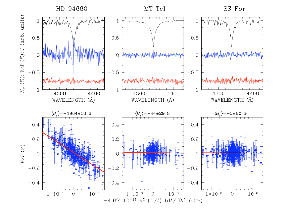
Figure 1: Spectropolarimetric observations of the magnetic star HD 94669 (left panels) and two program RR Lyrae stars (MT Tel, middle panels, and SS For, right panel). The top panels show the spectral region around H$\gamma$. The top, solid lines represent Stokes $I$, expressed in arbitrary units (and not normalized to the continuum); middle lines show the $P_{V}$ profiles, and the bottom lines show the null profile $N_{V}$, which represents an overal estimate of the noise of our circular polarization measurements. The bottom panels show the corresponding best fits to the full spectrum obtaining by minimizing the $\chi^{2}$ of Eq. (3).

3 Determinations of the mean longitudinal magnetic field

Our determinations of the mean longitudinal field $\langle B_{z}\rangle$  i.e., the component of the magnetic field along the line of sight, averaged over the stellar disk, are based on the use of the formula

$$\frac{V}{I}=-g_{\mathrm{eff}}\ C_{z}\ \lambda^{2}\ \frac{1}{I}\ \frac{\mathrm{d}I}{\mathrm{d}\lambda}\ \langle B_{z}\rangle\;,$$ (1)

where $g_{\mathrm{eff}}$ is the effective Landé factor and

$$C_{z}=\frac{e}{4\pi m_{\mathrm{e}}c^{2}}\ \ \ \ \ (\simeq 4.67\times 10^{-13}\,\mathrm{\AA}^{-1}\ {\rm G}^{-1})\;,$$ (2)

where $e$ is the electron charge, $m_{\mathrm{e}}$ the electron mass, and $c$ the speed of light.

A least-squares technique was used to derive the longitudinal field via Eq. (1), by minimizing the expression

$$\chi^{2}=\sum_{i}\frac{(y_{i}-\langle B_{z}\rangle\,x_{i}-b)^{2}}{\sigma^{2}_{i}}$$ (3)

where, for each spectral point $i$, $y_{i}=(V/I)_{i}$, $x_{i}=-g_{\mathrm{eff}}C_{z}\lambda^{2}_{i}(1/I\ \times\mathrm{d}I/\mathrm{d}\lambda)_{i}$, and $b$ is a constant.

Note that Eq. (1) is strictly correct under the so-called weak field approximation, which, e.g., in the atmosphere of main sequence A-type stars, is valid for field strengths $\la 1$ kG for metal lines, and up to $\sim 10$ kG for H lines.

Using low resolution spectra such as those obtained in this work, it would make sense to hypothesize that only broad H Balmer lines could be used to determine the magnetic field, since most metal lines are not resolved in the spectra. However, Bagnulo et al. (2002) and Bagnulo et al. (2006) have shown that Eq. (1) may also be applied to spectral regions with non resolved metal lines, leading to results consistent to the $\langle B_{z}\rangle$ determinations obtained on H Balmer lines in the weak field regime. We checked that with our spectra the $\langle B_{z}\rangle$ determination obtained from metal lines only are consistent, within the error bars, with the $\langle B_{z}\rangle$ values obtained from Balmer lines only. For Balmer lines we adopted an effective Landé factor of 1 (Casini & Landi Degl’Innocenti 1994); for metal lines, following Chadid et al. (2004), we used an effective Landé factor of 1.38. Finally, we applied the least-square technique to the full spectrum, i.e., using both metal and Balmer lines. This method allowed us to bring the $\langle B_{z}\rangle$ error bars down to a typical level of 20–30 G.

Similarly to the application by Bagnulo et al. (2006), the $\langle B_{z}\rangle$ values were determined using the $P_{V}$ profile obtained from the combinations of all exposures. For the purpose of checking our results, we also calculated the average of the $\langle B_{z}\rangle$ values obtained from individual pairs of exposures for each star, always finding results consistent with the $\langle B_{z}\rangle$ value obtained from the combined $P_{V}$ and $I$ profiles.

Since FORS1 is not equipped with circular polarization filters that allow one to routinely check the correct alignment of the polarimetric optics, and no standard stars for circular polarization are available, we decided to perform a health check by observing the well known magnetic Ap star HD 94660 (=KQ Vel=HIC 53379) during our observing run. Two consecutive series of eight observations were obtained, one with a 0.5″ slit width, and one with a 1.0″ slit width, using the same strategy adopted for the program stars. HD 94660 presents a roughly constant longitudinal magnetic field, and the measured value of $\sim-1960$ G (from Balmer lines only) is in reasonably good agreement with previous observations (see, e.g., Fig. 3 of Bagnulo et al. 2006, the new observation presented in this paper would be located at phase 0.96.).

Figure 1 shows our observations of stellar spectra in circular polarization, and their interpretation in terms of magnetic field for HD 94660, a known magnetic star, and two representative RR Lyrae stars: MT Tel, an RRc star, and SS For, an RRab Blazhko star. Note that the hotter RRc star clearly has less metal lines in its spectrum than the RRab star. The bottom panels show the best fits to the full spectrum obtained through minimizing the $\chi^{2}$ of Eq. (3). Whereas a clear slope is observed in the case of HD 94660, corresponding to the mean longitudinal magnetic field $\langle B_{z}\rangle$ , for the RR Lyrae stars the best fit results are consistent with a curve with no significant slope.

The results of our survey are reported in Table 2. Inspection of this table show that in all cases our $\langle B_{z}\rangle$ measurements are, within 3$\sigma$, fully consistent with a null detection of the mean longitudinal magnetic field. In other words, for the 17 stars in our sample and the 20 measurements taken, we obtained no field that differed from zero exceeding the 3 $\sigma$ significance level. In fact, 14 of our 20 measurements were null detections within a 1$\sigma$ significance level. A histogram reflecting our measurements is given in Fig. 2.

Table 2: Determination of the mean longitudinal magnetic field of 17 RR Lyrae stars.

Object	Type	Date	Time (UT) (1)	Exp (2)	Slit	$\phi$ (3)	$\psi$ (4)	$\langle B_{z}\rangle$		(SNR) (5)
		(yyyy mm dd)	(hh:mm)	(sec)	width	($\pm$0.02)		(G)
WZ Hya	RRab	2008 11 12	08:32	1920	0.5″	0.99	-	32 $\pm$	21	2620
V Ind	RRab	2008 11 13	03:03	2400	1.0″	0.89	-	$-$57 $\pm$	28	2820
U Lep	RRab	2008 11 11	05:06	2340	0.5″	0.23	-	$-$15 $\pm$	19	2930
RU Scl	RRab	2008 11 11	02:26	3900	0.5″	0.63	-	6 $\pm$	14	2865
CS Eri	RRc	2008 11 12	02:36	960	0.5″	0.41	-	3 $\pm$	19	3025
		2008 11 13	06:10	360	0.5″	0.10	-	5 $\pm$	22	2900
MT Tel	RRc	2008 11 11	00:10	1800	0.5″	0.07	-	$-$44 $\pm$	29	3370
RV Cap	RRab-BL	2008 11 13	01:56	4000	1.0″	0.17	0.4$\pm$0.1	$-$4 $\pm$	31	2640
RX Cet	RRab-BL	2008 11 12	03:41	4560	0.5″	0.92	*	45 $\pm$	21	1970
RV Cet	RRab-BL	2008 11 11	06:03	2880	0.5″	0.31	0.0$\pm$0.2	$-$6 $\pm$	15	2535
RX Col	RRab-BL	2008 11 11	07:24	4800	1.0″	0.19	0.5$\pm$0.2	$-$99 $\pm$	45	1480
RY Col	RRab-BL	2008 11 11	03:53	4700	1.0″	0.28	0.2$\pm$0.1	18 $\pm$	23	3020
VW Dor	RRab-BL	2008 11 12	07:35	3360	1.0″	0.27	*	$-$38 $\pm$	28	2270
SS For	RRab-BL	2008 11 11	01:12	3440	0.5″	0.61	0.43$\pm$0.10	2 $\pm$	19	2930
		2008 11 12	06:41	1440	0.5″	0.09	0.47$\pm$0.10	$-$5 $\pm$	20	2710
		2008 11 13	04:14	1440	0.5″	0.90	0.49$\pm$0.10	$-$16 $\pm$	30	1875
RX For	RRab-BL	2008 11 13	05:17	4413	1.0″	0.64	0.8$\pm$0.4	15 $\pm$	34	1855
SZ Hya	RRab-BL	2008 11 11	08:40	1920	0.5″	0.16	*	21 $\pm$	25	2160
X Ret	RRab-BL	2008 11 12	05:16	4800	1.0″	0.76	0.9$\pm$0.2	$-$4 $\pm$	29	2250
BV Aqr	RRc-BL	2008 11 12	01:46	3360	1.0″	0.44	*	6 $\pm$	27	3620
HD 94660	Magnetic Ap	2008 11 12	09:01	56	0.5″			$-$1831 $\pm$	15	3280
		2008 11 12	09:08	28	1.0″			$-$1872 $\pm$	25	3071
(1) The epoch of the observations refers to the middle of the eight exposures, and (2) the exposure time refers to the sum of eight exposures.
(3) $\phi$: pulsation phase; (4) $\psi$: Blazhko phase. The symbol ‘–’ is used for non-Blazhko stars. The symbol ‘*’ is used for Blazhko stars for which
the Blazhko phase could not be obtained with an error smaller than 0.5.
(5) The signal-to-noise ratio (SNR) is calculated per Å, in the wavelength interval 4475–4525 Å.

4 Discussion

4.1 The magnetic model challenged

The presence of a strong dipole magnetic field is a key ingredient for the model proposed by Shibahashi & Takata (1995) and Shibahashi (2000). Assuming that RR Lyrae stars have fairly strong dipole fields, Shibahashi (2000) showed that the radial mode in RR Lyrae stars would be deformed by the Lorenz force to have additional quadrupole ($\ell=2$) pulsation components. The changing aspect angle as a consequence of the rotation of a star would then give rise to an apparent amplitude variation. The quadrupole components induced by the magnetic field would give rise to a quintuplet structure in the frequency spectrum. For more than a decade after the magnetic model was first presented, no evidence for quintuplet components was found from any data set. Shibahashi & Takata (1995) showed that a quintuplet structure may manifest itself as only a triplet depending on the geometrical configuration (angles of pulsation axis, magnetic axis and aspect angle). Also, the quintuplet components might have such a low amplitude that they are hidden in the noise of the frequency spectrum of time series data. The latter explanation was supported by recent findings from high-quality data sets by Hurta et al. (2008) in RV UMa, Jurcsik et al. (2008) in MW Lyr, and Kolenberg et al. (2008) in SS For, one of the stars in our sample. However, the detection of quintuplet structures does not imply that the magnetic model is the one to be preferred over the resonance model. Jurcsik et al. (2008a) and Kolenberg et al. (2008) also found evidence of even higher order multiplet components (septuplets, nonuplets) in the frequency spectra of Blazhko stars. These frequency structures have never explicitly been considered in any of the models proposed to explain the Blazhko effect.

Our sample of stars consisted of RR Lyrae stars with different pulsational properties: RRab, RRc stars, and modulated star of both types. In none of these stars a field exceeding a significance level of $3\sigma$ was detected.

For the magnetic field to have the effects described by Shibahashi & Takata (1995) and Shibahashi (2000), the presence of a dipole field with a strength of the order of 1 kG was assumed. In the following section we discuss what constraints our measurements set to the magnetic field strength and morphology of our sample of stars.

4.2 Constraints on the magnetic field

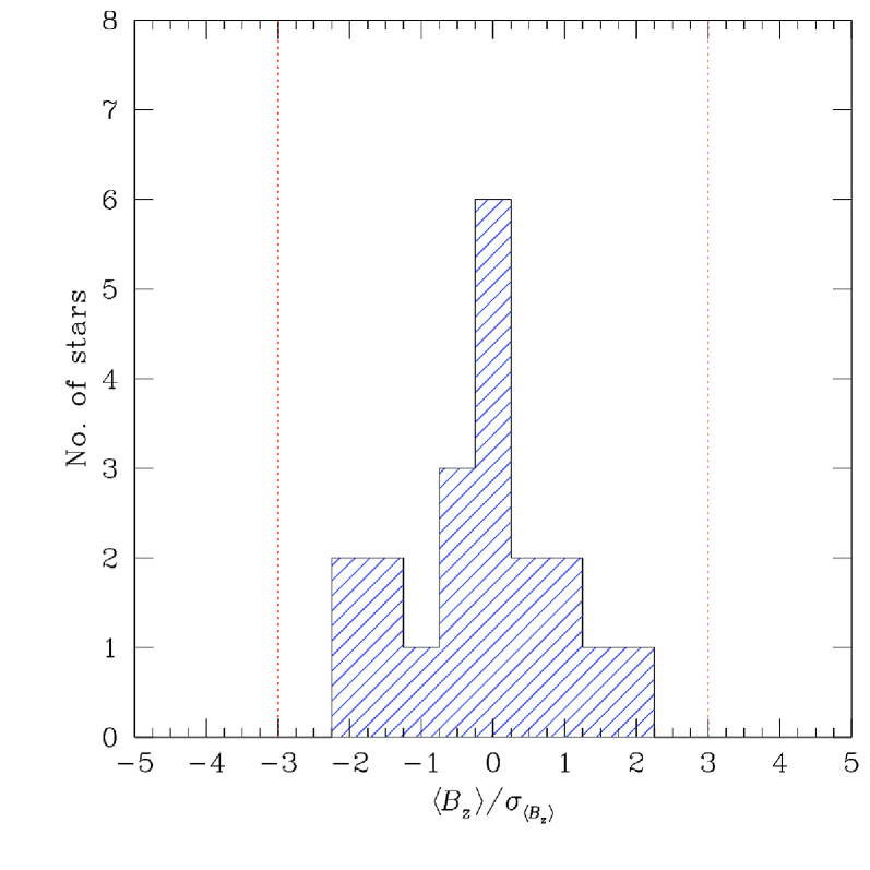
Figure 2: Distribution of the $\langle B_{z}\rangle$ values normalized to their error bars for our sample of 20 field measurements in 17 RR Lyrae stars. The dotted vertical lines correspond to the 3-$\sigma$ detection level.

We consider a magnetic configuration produced either by a dipole, or by a (non-linear) quadrupole, or by the superposition of both. The model is assumed to be centered, i.e. the elementary multipoles that produce the magnetic configuration at the stellar surface are located at the star’s center. The dipole field $\@vec{\mathcal{B}}_{\mathrm{d}}(\@vec{r})$ can be characterized by the dipole field strength $B_{\mathrm{d}}$ at the pole, plus the direction of a unit vector $\@vec{u}$; the quadrupole field $\@vec{\mathcal{B}}_{\mathrm{q}}(\@vec{r})$ can be characterized by the quadupole field strength $B_{\mathrm{q}}$, plus the directions of two unit vectors $\@vec{u}_{1}$ and $\@vec{u}_{2}$. The geometric configuration of a dipole plus quadrupole magnetic field is illustrated in Fig. 1 of Landolfi et al. (1998). Denoting by $R_{*}$ the star’s radius, the magnetic field vector at a given point $\@vec{r}$ of the stellar surface is given, respectively, by

$$\begin{array}[]{rcl}\@vec{\mathcal{B}}_{\mathrm{d}}(\@vec{r})&=&-\frac{B_{\mathrm{d}}}{2}\left[\,\@vec{u}-3\,\frac{\@vec{u}\cdot\@vec{r}}{R_{*}^{2}}\;\@vec{r}\,\right]\\[4.26773pt] \@vec{\mathcal{B}}_{\mathrm{q}}(\@vec{r})&=&-\frac{B_{\mathrm{q}}}{2}\left[\frac{\@vec{u_{2}}\cdot\@vec{r}}{R_{*}}\;\@vec{u_{1}}\,+\,\frac{\@vec{u_{1}}\cdot\@vec{r}}{R_{*}}\;\@vec{u_{2}}\right.\\[4.26773pt] &&\hphantom{-\frac{B_{\mathrm{q}}}{2}\biggl{[}}\left.+\left(\frac{\@vec{u_{1}}\cdot\@vec{u_{2}}}{R_{*}}-5\,\frac{(\@vec{u_{1}}\cdot\@vec{r})(\@vec{u_{2}}\cdot\@vec{r})}{R_{*}^{3}}\right)\@vec{r}\,\right]\ .\end{array}$$

Note that while the quantity $B_{\mathrm{d}}$, the dipole field modulus at the magnetic pole, has an obvious physical meaning, the quantity $B_{\mathrm{q}}$ represents the quadrupole field modulus at the magnetic pole only when the unit vectors $\@vec{u}_{1}$ and $\@vec{u}_{2}$ coincide (linear quadrupole), otherwise the concept itself of magnetic pole becomes meaningless, and the estimate of the actual field strength requires an evaluation of Eq. (4.2) for the specific quadrupole configuration. For a more detailed description of the multipolar expansion of the magnetic field see Bagnulo et al. (1996).

Assuming a limb-darkening law of the form

$$1-u+u\,\mu\ \ (0\leq u\leq 1)\;,$$ (4)

where $\mu$ is the cosine of the angle between the line of sight through the star disk center and a given point of the stellar disk, and using Eqs. (24), (28) and (68) of Bagnulo et al. (1996), we find that the mean longitudinal field is given by

$$\begin{array}[]{rcl}\langle B_{z}\rangle&=&\frac{3}{3-u}\,\Big{[}\frac{15\,+\,u}{60}B_{\mathrm{d}}\cos\ell\\ &+&\frac{u}{12}B_{\mathrm{q}}\big{(}\cos\ell_{1}\cos\ell_{2}+\frac{1}{2}\sin\ell_{1}\sin\ell_{2}\cos(\Lambda_{1}-\Lambda_{2})\big{)}\Big{]}\\ \end{array}$$ (5)

where $\ell$ is the angle between the line of sight and the dipole axis, $\ell_{1}$ and $\ell_{2}$ are the angles between line of sight and the unit vectors $u_{1}$ and $u_{2}$ that define the quadrupolar component of the magnetic field, and $\Lambda_{1}$ and $\Lambda_{2}$ are the azimuth angles of the same unit vectors, reckoned counterclockwise in the plane of the sky from the north celestial meridian, as detailed in Bagnulo et al. (1996).

Even a quick glance at the results in Table 2 tells us that, if a dipole field is present, its strength must be small, much smaller than the 1 kG field that the magnetic model (Shibahashi 2000) requires to be responsible for the Blazhko effect. Based on our measurements, it is possible to obtain more precise constraints on the magnetic field of our program stars.

Let us consider the case of a pure dipolar field. We assume that all stars of our sample have the same dipolar strength, and that the magnetic axis is randomly oriented with respect to the line of sight. The probability $P(\ell)$ for the tilt angle of the field $\ell$ to be in the range $[\ell,\ell+\mathrm{d}\ell]$ is proportional to $\sin\ell\mathrm{d}\ell$. A simple application of Bayesian statistics allows us to evaluate the probability $\mathcal{P}(B_{\mathrm{d}}\geq B_{\mathrm{d}}^{(0)})$ that all the observed stars of our sample are characterized by a dipolar field strength higher than a certain threshold value $B_{\mathrm{d}}^{(0)}$:

$$\begin{array}[]{l}\mathcal{P}(B_{\mathrm{d}}\geq B_{\mathrm{d}}^{(0)})\propto\\ \ \ \ \ \int\limits_{B_{\mathrm{d}}^{(0)}}^{+\infty}\,\mathrm{d}B_{\mathrm{d}}\ \ \prod\limits_{j=1}\limits^{N}\ \frac{1}{\sqrt{2\pi}\sigma_{j}}\,\int\limits_{0}^{\pi}\,\mathrm{d}\ell\sin\ell\,\exp{\left(-\frac{\big{(}\langle B_{z}\rangle_{j}-k(u)B_{\mathrm{d}}\cos\ell\big{)}^{2}}{2\,\sigma^{2}_{j}}\right)}\\ \end{array}$$ (6)

where the product runs on the $N=17$ observed stars (for the $\langle B_{z}\rangle$ value of the two stars that were observed more than once, we consider the value measured first), $\sigma_{j}$ is the error bar associated to the measurement of the $j^{\rm th}$ star, and we have set

$$k(u)=\frac{15+u}{20\,(3-u)}\ .$$ (7)

Using a limb-darkening coefficient $u=0.62$, derived from Diaz-Cordoves et al. (1995) (see also Kolenberg 2002), we obtain that if the RR Lyrae stars of our sample are all characterized by the same dipolar strength, with magnetic axis randomly oriented about the line of sight, then there is a 95 % probability that their dipolar strength is $\la 130$ G.

Equation (5) shows that, for the limb-darkening coefficient of $u=0.62$, the contribution of the quadrupolar component to the mean longitudinal magnetic field is always $\la 20$ % the contribution due to the dipolar component (assuming $B_{\mathrm{d}}$ = $B_{\mathrm{q}}$). For a linear quadrupole, i.e., with $\@vec{u_{1}}\parallel\@vec{u_{2}}$, we always have $\ell_{1}=\ell_{2}$ and $\Lambda_{1}=\Lambda_{2}$, and our observations rule out a quadrupolar field strength $\ga 250$ G at the 95 % confidence level. If we consider the special case where $\ell_{2}=\ell_{1}+90\degr$ and $\Lambda_{1}=\Lambda_{2}$ (for which $\@vec{u_{1}}\perp\@vec{u_{2}}$), we obtain the value $B_{\mathrm{q}}$= 1.9 kG as an upper limit to the quadrupole strength.

Therefore, determinations of the mean longitudinal field as obtained in this work set fairly loose constraints on the magnetic field strength for morphologies of higher order than the dipole field.

4.3 Variability over pulsation cycle and Blazhko cycle

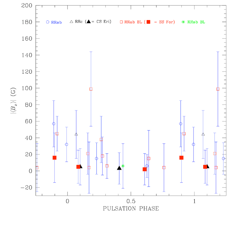
Figure 3: Absolute value of the mean longitudinal field versus pulsation phase. Different symbols were used for different types of RR Lyrae stars. Data points for stars observed more than once are denoted with filled symbols.

Figure 3 shows the plot of the absolute value of the mean longitudinal field as a function of the pulsation phase. Although this plot refers to different stars with different geometric configurations, it could potentially reveal the presence of a cyclic variability of the magnetic field over the pulsation cycle as was also observed on several nights by Romanov et al. (1987) (their Figs. 1 and 2). Indeed, Figure 3 shows a hint for higher $\langle B_{z}\rangle$ values (though all consistent with zero) close to phase zero. This could be explained by the presence of a small magnetic field and assuming magnetic flux conservation. (The stellar radius and surface is minimum shortly before phase zero, and attains its highest value around phase $\phi=0.5$.) Further conclusions may be drawn only after a detailed monitoring of individual stars.

For two of the stars in our sample, CS Eri (RRc) and SS For (RRab-BL), we obtained more than one measurement at different phases in their pulsation cycle. No clear variation with the pulsation phase exceeding the error bars could be derived for these stars. We observed SS For at 3 different phases: one at maximum light, a second one approaching minimum light, and a third one on the rising branch of the light variation. From the last spectrum a higher absolute $\langle B_{z}\rangle$ was derived, but also a higher error bar, which can be attributed to the lower signal-to-noise ratio of the spectrum. SS For shows quintuplets in its pulsation spectrum (Kolenberg et al. 2008) which, according to the magnetic model (Shibahashi 2000) are associated with the effects of a magnetic field (see also Section 4.1), and hence was one of our prime targets for investigating the presence of a magnetic field.

Romanov et al. (1987) also reported a variation of their derived mean longitudinal magnetic field values over the Blazhko cycle of RR Lyr. Chadid et al. (2004), in contrast, with 27 measurements of the same star, detected no significant changes at different Blazhko phases. Within the allocated telescope time we were not able to follow one Blazhko star at different Blazhko phases. Only for some stars in our sample the Blazhko phase could be determined with a reasonable accuracy. However, we can safely say that the 11 Blazhko stars in our sample were recorded at random Blazhko phases, and for all of them we obtained a mean longitudinal magnetic field consistent with a null detection within $3\sigma$. As discussed in Section 4.2, this implies low values for the magnetic dipole field.

Our observations significantly enlarge the sample of spectropolarimetric measurements of RR Lyrae stars and follow the line of results obtained by Preston (1967) and Chadid et al. (2004). The latter authors declared RR Lyr to be a bona fide non-magnetic star on the basis of high-resolution spectropolarimetric data obtained over a 4-year time span.

Now why did earlier measurements of the magnetic field in specifically RR Lyr, the brightest star of the class, lead to reported values of the longitudinal magnetic field strength as high as about 1.5 kG (Babcock 1958; Romanov et al. 1987), while more recent observations contradict this? Chadid et al. (2004) addressed this question in the necessary detail (in their Section 3.1), pointing at the limitations of the use of photographic plates resulting in underestimated error bars, and the distortions of the spectral lines caused by shock waves in certain pulsation phases (see also Wade et al. 2002). The measurement with by far the highest $\langle B_{z}\rangle$ detection by Romanov et al. (1987) was recorded at the phase of the main shock in the star ($\phi$=0.95). This may have led to spurious polarization signals. We also note two limiting factors of those earlier measurements: i) a quite low reciprocal dispersion (9Å/mm) of their plate material, which is possibly not sufficient to perform high accuracy splitting measurements of the spectral lines observed in opposite polarization; ii) the employment of the Nasmyth focus station for the polarimeter: the oblique reflection from the tertiary mirror is prone to introduce a spurious polarization signal. This problem is much less critical at the Cassegrain focus, which was used instead for both the MuSiCoS observations obtained by Chadid et al. (2004), and the FORS1 measurements presented in this work. We therefore suggest that the magnetic field in RR Lyr was significantly overestimated in the earlier studies.

5 Conclusion

The results of our survey of magnetic fields in RR Lyrae stars reveal a serious challenge to the magnetic models for explaining the Blazhko effect. For a sample consisting of 17 RR Lyrae stars with different pulsational properties, no substantial dipole magnetic field, as required by the magnetic model (Shibahashi 2000), was detected. We determined an upper limit for the strength of the dipole field in the stars of our sample at 130 G with a 95% confidence level. Our result implies that the Blazhko modulation in the pulsation of RR Lyrae stars is not correlated with the presence of a strong, quasi-dipolar magnetic field. For morphologies of higher order than the dipole field, however, our determinations of the mean longitudinal field as obtained in this work only set fairly loose constraints on the magnetic field strength. More complex magnetic field morphologies may be detected with high-resolution spectropolarimetric data.