Conservation laws for voter-like models on directed networks

Abstract

We study the voter model, under node and link update, and the related invasion process on a single strongly connected component of a directed network. We implement an analytical treatment in the thermodynamic limit using the heterogeneous mean field assumption. From the dynamical rules at the microscopic level, we find the equations for the evolution of the relative densities of nodes in a given state on heterogeneous networks with arbitrary degree distribution and degree-degree correlations. We prove that conserved quantities as weighted linear superpositions of spin states exist for all three processes and, for uncorrelated directed networks, we derive their specific expressions. We also discuss the time evolution of the relative densities that decay exponentially to a homogeneous stationary value given by the conserved quantity. The conservation laws obtained in the thermodynamic limit for a system that does not order in that limit determine the probabilities of reaching the absorbing state for a finite system. The contribution of each degree class to the conserved quantity is determined by a local property. Depending on the dynamics, the highest contribution is associated to influential nodes reaching a large number of outgoing neighbors, not too influenceable ones with a low number of incoming connections, or both at the same time.

I Introduction

Conservation laws are intimately related to symmetries in the systems they hold for. They play an important role in the characterization and classification of different nonequilibrium processes of ordering dynamics. For example, in Kinetic Ising models one distinguishes between Glauber (spin flip) and Kawasaki (spin exchange) dynamics. Kawasaki dynamics fulfils a microscopic conservation law, such that the total magnetization is conserved in each individual dynamical step of a stochastic realization. This conservation law does not hold for Glauber As a consequence, the Glauber and Kawasaki dynamics give rise to different scaling laws for domain growth in coarsening processes Gunton et al. (1983), and they define different nonequilibrium universality classes.

In other types of nonequilibrium lattice models non-microscopic conservation laws are known to hold. They are statistical conservation laws in which the conserved quantity is an ensemble average defined over different realizations of the stochastic dynamics for the same distribution of initial conditions. Examples of such conservation laws occur for the voter model Clifford and Sudbury (1973); Holley and Liggett (1975) or the invasion process Castellano (2005). In particular, the role of the conservation law of the magnetization and of the $Z_{2}$ symmetry ( 1 states) in the voter dynamics universality class has been studied in detail in the critical dimension d = 2 of regular lattices Dornic et al. (2001). The voter model is a paradigmatic model of consensus dynamics in the social context San Miguel et al. (2005); Castellano et al. (2008) or, in the biological context, of competition of plant species in ecological communities Chave (2001). In general, any Markov chain with at least two absorbing states reachable from all other configurations has a conserved quantity when averaged over the ensemble. Such a quantity determines the probability to eventually reach a particular absorbing configuration in a finite system. In some cases, this conservation law is of rather trivial nature as in the zero temperature Ising Glauber dynamics where the magnetization sign is conserved. The voter model, the zero temperature Ising Glauber dynamics, and other related models of language evolution Castelló et al. (2006) or population dynamics Tilman and Kareiva (1997), belong to the class of models with two absorbing states while epidemic spreading dynamics, like the contact process Boguñá et al. (2008) or the Susceptible-Infected-Susceptible model Pastor-Satorras and Vespignani (2001), usually have a single absorbing state with no conservation law.

While some of these questions have been studied for spin lattice models for a long time, conservation laws for dynamical processes on complex networks Albert and Barabási (2002); Dorogovtsev and Mendes (2003); Newman (2003); Barrat et al. (2008) still remain a challenge. This issue has been considered for the voter model Clifford and Sudbury (1973); Holley and Liggett (1975) or the invasion process Castellano (2005) on undirected uncorrelated networks Wu and Huberman (2004); Suchecki et al. (2005a); Sood et al. (2008); Vazquez and Eguíluz (2008). The link-update dynamics for the voter model has been found to conserve the global magnetization Suchecki et al. (2005b), while the node update dynamics Suchecki et al. (2005b) and the invasion process Sood et al. (2008) preserve a weighted global magnetization where the contribution of each spin is calibrated by some function of the degree of the corresponding node in the undirected network. Such ensemble average conservation laws characterize processes with two absorbing states accessible to the dynamics, that compete to maintain an active state in the thermodynamic limit. In finite networks, the conserved quantities give the probabilities of reaching the uniform states and so act as a bridge that enables some probabilistic predictive power of the final dynamical state based on information about the initial conditions. In addition, different finite size dynamical scaling properties can be related to different conservation laws Suchecki et al. (2005b).

Much less has been done exploring dynamical processes on directed networks, with the exception of the Ising model Sánchez et al. (2002) and Boolean dynamics mainly applied to biological problems Kauffman (1969). However, interactions between pairs of elements are asymmetric in different systems including some social networks Newman (2001), where social ties are perceived or implemented differently by the two individuals forming the connected pairs. Directed network representations rather than undirected ones become more informative and adjusted to reality. In general, directed networks present characteristic large-scale connectivity structures, the so-called bow-tie architecture formed by a strongly connected component as a core structure and peripheral in- and out-components Broder et al. (2000). This organization, coupled to the initial condition of the dynamics running on top, have an impact both on the evolution of the processes and the final possible states of the systems Lieberman et al. (2005); Park and Kim (2006); Jiang et al. (2008). In the voter model, leaf nodes in the in-component never change their state thus sending an invariable signal that can potentially propagate to the rest of the components of the system. This is closely related to phenomena such as the presence of zealots Mobilia (2003); Mobilia et al. (2007) in undirected networks. Both input or output directional large-scale components and zealotry imply at the end an external forcing on the dynamical processes that prevents reaching one of the absorbing states even for a finite network. This is clearly illustrated by the evolution of dynamical processes running on networks at the transition from a pure strongly connected component to a complete bow-tie structure. In an isolated and strongly connected component, the voter dynamics keeps an active dynamical state in the thermodynamic limit, but it leads to a consensus (absorbing state) in a finite network as it happens on undirected networks. Thus, the appearance of an input component in the large-scale structure of the network prevents the system from reaching an absorbing state for random initial conditions Park and Kim (2006).

In this paper, we focus on dynamics of coupled two-state spin variables and consider conserved quantities that are weighted sums of the spin values. Specifically, we investigate the form of the conservation law for the voter model — under node and link update — and the invasion process in directed networks with arbitrary degree distribution and degree-degree correlations. The directionality of the interactions is therefore encoded in the topology. We restrict to a single strongly connected component so that the absorbing state can be reached in a finite system, what seems realistic for a number of densely connected real networks like the world trade web Serrano et al. (2007). In Sec. II, we present a detailed study of the node update version of the voter model and implement an analytical treatment using the heterogeneous mean field assumption in the thermodynamic limit. From the dynamical rules at the microscopic level, we find the equations for the evolution of the relative densities of nodes in one of the two possible states on heterogeneous networks with arbitrary degree distribution and degree-degree correlations. In this case, we prove that a conserved quantity as a weighted linear superposition of spin states exists. In Sec. III, we discuss the node-update voter model in uncorrelated directed networks to derive analytical expression for the conservation law and we also discuss the exponential decay of the relative densities to their homogeneous stationary value, which is basically a function of the conserved quantity. We show how the conserved quantity determines the probability of reaching one of the two states in a finite network. In Sec. IV and V, we present the results of applying the same methodology to the voter model with link update and the invasion process, respectively. We conclude in Sec. VI with a summary of results and open questions for future research.

II The voter model on strongly connected components

In the voter model under node update (VM), each node of a network can exist in one of two possible states, $1$ or $0$ . In a single dynamical event, a randomly selected node copies the state of one of its neighbors, also selected at random. The link update dynamics of the Voter model selects instead a link Suchecki et al. (2005b). Time is increased by $1/N$, so that the physical time is incremented by 1 after $N$ of such events. On undirected networks, the node-update voter model conserves the ensemble average of a weighted magnetization, where the contribution of each spin is multiplied by the degree of the corresponding node.

As defined above, the interactions in the voter dynamics are instantaneously asymmetric since the updates always go in the same direction once the original node is chosen independently of the undirectionality of the substrate. Hence, the discussion of the voter model on directed networks comes out as a natural one, where the directionality of the interaction is decoupled from the dynamics and encoded in the structure of the substrate. The straightforward generalization of the voter model on directed networks under node update consists of selecting a node at random, and then assigning to it the state of one of its incoming neighbors, also chosen at random. We will discuss this dynamics next in this section and Sec. III, and the voter model with link update will be discussed later in Sec. IV.

II.1 Directed networks

The topological structure of directed networks is more complex than the one of undirected graphs. In purely directed networks, without bidirectional links, the edges are differentiated into incoming and outgoing, so that each vertex has two coexisting degrees $k_{\textrm{in}}$ and $k_{\textrm{out}}$, with total degree $k=k_{\textrm{in}}+k_{\textrm{out}}$. Hence, the degree distribution for a directed network is a joint degree distribution $P(k_{\textrm{in}},k_{\textrm{out}})\equiv P({\bf k})$ of in- and out-degrees that in general may be correlated. We consider degree correlations $P_{\textrm{in}}({\bf k^{\prime}}|{\bf k})$ and $P_{\textrm{out}}({\bf k^{\prime}}|{\bf k})$, which respectively measure the probability to reach a vertex of degree ${\bf k^{\prime}}$ leaving from a vertex of degree ${\bf k}$ using an incoming or outgoing edge of the source vertex, and are related through the following degree detailed balance condition Boguñá and Serrano (2005)

$$k_{\textrm{out}}P({\bf k})P_{\textrm{out}}({\bf k^{\prime}}|{\bf k})=k^{\prime}_{\textrm{in}}P({\bf k^{\prime}})P_{\textrm{in}}({\bf k}|{\bf k^{\prime}}).$$ (1)

This ensures that the network is closed and $\left<k_{\textrm{in}}\right>=\left<k_{\textrm{out}}\right>$. Apart from the prescribed degrees and two point correlations, networks are maximally random.

At the macroscopic scale, the giant weakly connected component, i.e., the set of nodes that can communicate to each other when considering the links as undirected Molloy and Reed (1995, 1998); Cohen et al. (2000); Callaway et al. (2000); Newman et al. (2001), becomes internally structured in three giant connected components, as well as other secondary structures such as tubes or tendrils, forming a bow-tie architecture Broder et al. (2000). The main component is the strongly connected component (SCC), a central core formed by the set of vertices that can be reached from each other following a directed path. The other two main components are peripheral components, the in component (IN) formed by all vertices from which the SCC is reachable by a directed path but that cannot be reached from there, and the out component (OUT) formed by all vertices that are reachable from the SCC by a directed path but cannot reach the SCC themselves. Percolation theory for purely directed networks was first developed for uncorrelated networks Callaway et al. (2000); Newman et al. (2001); Dorogovtsev et al. (2001a, b); Serrano and De Los Rios (2007), and directed random networks with arbitrary two point degree correlations and bidirectional edges Boguñá and Serrano (2005).

We restrict to networks forming a strongly connected component without peripheral components that would act on the SCC as sources of external forcing. We will see that within the strongly connected component, conservation laws preserve weighted magnetizations, where the weights are dictated by the directed degrees.

II.2 From microscopic dynamics to the drift equation under the heterogeneous mean field assumption

To study the time evolution of the system, we consider the drift part of the Langevin equation for the density of nodes in one of the states from a microscopic description of the evolution of single nodes’ states applying a heterogeneous mean field approach. To our knowledge, this methodology, which allows us to deal with dynamical processes on complex networks, was first presented in Refs. Catanzaro et al. (2005, 2008) and recently used to study the contact process Boguñá et al. (2008). In Vazquez et al. (2008); Vazquez and Eguíluz (2008), a homogeneous mean field pair approximation was instead developed.

We focus on the microscopic state of nodes at some time $t$. Let $s_{u}(t),u=1,...,N$, be a stochastic binary variable defined for each of the $N$ nodes in the network which describes its state, $0$ or $1$. The vector ${\bf s}(t)\equiv\{s_{u}(t)\},u=1,\ldots,N$, completely defines the dynamical state of the system at time $t$. Two more independent binary stochastic variables $\mu(dt)$ and $\xi_{u}$ are defined in order to model the transitions between states of single nodes in an iteration. After a time interval $dt$, the variable $\mu(dt)$ for a given node $u$ takes the value $1$ or $0$ if $u$ was chosen or not, respectively. In case node $u$ was selected, then $\xi_{u}$ assumes the value 1 [0] if $u$ copies a neighbor with state 1 [0]. We assume that the occurrence of events in the voter dynamics follows an independent Poisson process for each node, with constant rate $\lambda$ for all of them, which corresponds to a Montecarlo step. In the remainder we be set to $\lambda=1$ without loss of generality. Thus, $\mu(dt)$ and $\xi_{u}$ have probability distributions

$$P(\mu(dt))=dt\delta_{\mu(dt),1}+(1-dt)\delta_{\mu(dt),0},$$ (2)

$$P(\xi_{u})=\Phi_{u}/k_{u,\textrm{in}}\delta_{\xi_{u},1}+(1-\Phi_{u}/k_{u,\textrm{in}})\delta_{\xi_{u},0},$$ (3)

where $k_{u,\textrm{in}}$ is the incoming degree of node $u$, and we have defined $\Phi_{u}(t)=\sum_{v}a_{vu}s_{v}(t)$. The adjacency matrix $\{a_{vu}\}$ encodes the topological properties of the directed network. Element $a_{vu}$ has value one if there is a directed link from $v$ to $u$ and zero otherwise, so that $\Phi_{u}(t)$ stands for the number of state-one incoming neighbors of node $u$ at time $t$. The matrix $\{a_{vu}\}$ is symmetric for undirected networks but for directed ones it is in general asymmetric.

In terms of the above variables, the dynamical state $s_{u}(t)$ of node $u$ after an increment of time $dt$ is

$$s_{u}(t+dt)=\mu(dt)\xi_{u}+(1-\mu(dt))s_{u}(t).$$ (4)

This equation, together with Eqs. (2) and (3), give the complete description of the evolution of the system, making the formalism general and applicable to any network structure.

Although exact, this microscopic description is unmanageable. In order to reduce the degrees of freedom, we apply a heterogeneous mean-field hypothesis Pastor-Satorras and Vespignani (2001) so that nodes with the same degree ${\bf k}$ are assumed to be statistically independent and equivalent and can be aggregated in the same degree class $\Upsilon({\bf k})\equiv\Upsilon(k_{\textrm{in}},k_{\textrm{out}})$. Properties are then defined for each degree class, that will be characterized by the relative density $m_{\bf k}(t)$, the ratio between the number of state-one nodes within class $\Upsilon({\bf k})$ and its number of nodes $N_{\bf k}$,

$$m_{\bf k}(t)=\frac{\sum_{u\epsilon\Upsilon({\bf k})}s_{u}(t)}{N_{\bf k}}.$$ (5)

In the thermodynamic limit, the relative densities $m_{\bf k}(t)$ can be considered as continuous variables. Their time evolution can be described by a Langevin equation Gardiner (2004) with drift and diffusion coefficients that are respectively given by the first and second infinitesimal moments of the stochastic variables $m_{\bf k}(t)$. Those moments can be derived from the microscopic equation Eq. (4) along with the definition in Eq. (5). In the thermodynamic limit, it is possible to prove that the diffusion term has a dependence $1/\sqrt{N_{k}}$ on the system size as for undirected networks Vazquez and Eguíluz (2008), so that the drift term $A_{k}$ will dominate. It is given by the average value over all possible configurations of $m_{\bf k}(t+dt)$ conditioned to the state of the system at time $t$,

$$\left<m_{\bf k}(t+dt)\right>_{m_{\bf k}(t)}=m_{\bf k}(t)+A_{k}(t)dt.$$ (6)

From the microscopic dynamics

$$\left<s_{u}(t+dt)\right>_{{\bf s}(t)}=s_{u}(t)-dt\left[s_{u}(t)-\Phi_{u}(t)/k_{u,\textrm{in}}\right],$$ (7)

and summing this equation for all nodes in the degree class ${\bf k}$ and dividing by the number of nodes $N_{\bf k}$, we arrive to

$$\left<m_{\bf k}(t+dt)\right>_{m_{\bf k}(t)}=m_{\bf k}(t)-dt\left[m_{\bf k}(t)-\frac{1}{N_{\bf k}}\frac{1}{k_{\textrm{in}}}\sum_{u\epsilon\Upsilon({\bf k})}\Phi_{u}(t)\right],$$ (8)

and from here to

$$A_{k}(t)=-m_{\bf k}(t)+\frac{1}{N_{\bf k}}\frac{1}{k_{\textrm{in}}}\sum_{u\epsilon\Upsilon({\bf k})}\Phi_{u}(t).$$ (9)

The adjacency matrix contained in $\Phi_{u}(t)$ can be coarse-grained as well, so that a differential equation for the relative densities can eventually be written. This coarse-graining restricts the validity of the equations to random complex networks (and not lattices), since we assume all nodes in the same degree class to be statistically independent. With these assumptions,

$$\sum_{u\epsilon\Upsilon({\bf k})}\Phi_{u}(t) = \sum_{\bf k^{\prime}}\sum_{v\epsilon\Upsilon({\bf k^{\prime}})}\sum_{u\epsilon\Upsilon({\bf k})}a_{vu}s_{v}(t)$$ (10)

$$= \sum_{\bf k^{\prime}}\bar{a}_{\bf k^{\prime}k}N_{\bf k}N_{\bf k^{\prime}}m_{\bf k^{\prime}}(t).$$

At this point, we restrict to directed networks organized at the large scale into a SCC without IN and OUT. This allows us to write

$$\bar{a}_{\bf k^{\prime}k}=\frac{E_{\bf k^{\prime}k}}{N_{\bf k}N_{\bf k^{\prime}}}=\frac{k^{\prime}_{\textrm{out}}P_{\textrm{out}}({\bf k}|{\bf k^{\prime}})}{N_{\bf k}}=\frac{k_{\textrm{in}}P_{\textrm{in}}({\bf k^{\prime}}|{\bf k})}{N_{\bf k^{\prime}}},$$ (11)

where $E_{\bf k^{\prime}k}$ is the asymmetric matrix of the number of connections from the class of vertices of degree ${\bf k^{\prime}}$ to the class of vertices of degree ${\bf k}$, and where we have made use of the detailed balance condition Eq. (1).

Inserting these results into Eq. (9), we arrive to the equation for the evolution of the relative density in the degree class ${\bf k}$ of a purely directed correlated network (disregarding diffusion terms),

$$\frac{dm_{\bf k}(t)}{dt}=-m_{\bf k}(t)+\sum_{\bf k^{\prime}}P_{\textrm{in}}({\bf k^{\prime}}|{\bf k})m_{\bf k^{\prime}}(t).$$ (12)

Let us recall that this result is valid for the ensemble of networks defined by the degree distribution $P({\bf k})$ and the degree correlations $P_{\textrm{in}}({\bf k^{\prime}}|{\bf k})$ and $P_{\textrm{out}}({\bf k^{\prime}}|{\bf k})$, but otherwise maximally random. Notice that big enough networks present good statistical quality at the level of degree classes and are also well described by this equation. Finally, in the thermodynamic limit, the Langevin equation loses its noise term because of the dependence on the system size and reduces to Eq. (12), so that $m_{\bf k}(t)$ becomes a deterministic variable. Nevertheless, since the process is linear, Eq. (12) is always valid even for finite systems understanding that in this case the variables are averages over realizations of the process with the same distribution of initial conditions.

II.3 Conserved quantity on directed networks with degree-degree correlations

For correlated networks, $m_{\bf k}(t)=\sum_{\bf k^{\prime}}P_{\textrm{in}}({\bf k^{\prime}}|{\bf k})m_{\bf k^{\prime}}(t)$ in the stationary state and hence all relative densities are entangled through topological correlations. This equation corresponds indeed to an eigenvector problem, since $\{m_{\bf k}(t)\}$ can be thought as the eigenvector of the matrix $\{P_{\textrm{in}}({\bf k^{\prime}}|{\bf k})\}$ with eigenvalue one.

We prove next that, within the heterogeneous mean field approach and for the correlated directed networks we are considering, there is a conserved quantity given as a linear superposition of the form $\omega=\sum_{\bf k}\varphi_{\bf k}m_{\bf k}(t)$. From Eq. (12), its evolution is given by

$$\frac{d\omega}{dt}=-\omega+\sum_{\bf k}\sum_{\bf k^{\prime}}\varphi_{\bf k}P_{\textrm{in}}({\bf k^{\prime}}|{\bf k})m_{\bf k^{\prime}}(t),$$ (13)

and imposing that $d\omega/dt=0$, we obtain

$$\sum_{\bf k}\varphi_{\bf k}m_{\bf k}(t)=\sum_{\bf k}\sum_{\bf k^{\prime}}P_{\textrm{in}}({\bf k}|{\bf k^{\prime}})\varphi_{\bf k^{\prime}}m_{\bf k}(t).$$ (14)

For each density

$$\varphi_{\bf k}=\sum_{\bf k^{\prime}}P_{\textrm{in}}({\bf k}|{\bf k^{\prime}})\varphi_{\bf k^{\prime}}.$$ (15)

This is an eigenvector equation that has a solution if the matrix $\{P_{\textrm{in}}({\bf k}|{\bf k^{\prime}})\}$ has an eigenvalue equal to one with $\{\varphi_{\bf k}\}$ the corresponding eigenvector. One can prove that this eigenvector with eigenvalue one exists by summing both sides of the previous equation over ${\bf k}$. Using the normalization of the conditional probability $\sum_{\bf k}P_{\textrm{in}}({\bf k}|{\bf k^{\prime}})=1$, one eventually arrives to a trivial identity . The fact that the coefficients $\varphi_{\bf k}$ that modulate the contributions of the different $m_{\bf k}$ to the conserved weighted magnetization correspond to the entries of the eigenvector of a certain characteristic matrix with eigenvalue one also applies to other similar dynamical processes, such as the link dynamics and the invasion process, as we will show.

This proves that a conserved quantity of the form of a linear functional exists but, in general, it is not possible to derive its value without further specifying the form of the degree-degree correlations in the network.

III Voter model on uncorrelated SCCs

When two-point correlations are absent, the transition probabilities become independent of the degree of the source vertex. In this situation,

$$P_{\textrm{out}}({\bf k^{\prime}}|{\bf k})=\frac{k^{\prime}_{\textrm{in}}P({\bf k^{\prime}})}{\langle k_{\textrm{in}}\rangle}\mbox{ , }P_{\textrm{in}}({\bf k^{\prime}}|{\bf k})=\frac{k^{\prime}_{\textrm{out}}P({\bf k^{\prime}})}{\langle k_{\textrm{in}}\rangle},$$ (16)

and using these expressions, Eq. (12) becomes

$$\frac{dm_{\bf k}(t)}{dt}=-m_{\bf k}(t)+\omega_{\textrm{out}},$$ (17)

where we have defined

$$\omega_{\textrm{out}}=\frac{1}{\left<k_{\textrm{in}}\right>}\sum_{\bf k}k_{\textrm{out}}P({\bf k})m_{\bf k}(t).$$ (18)

Therefore, in the stationary state $m_{\bf k}=\omega_{\textrm{out}}\mbox{ }\forall{\bf k}$ and $\omega_{\textrm{out}}$ is a conserved quantity in uncorrelated networks, which immediately follows from Eq. (17). In general, it is not preserved in strongly connected components of directed networks with degree-degree correlations. This is in contrast to undirected networks, where the conserved quantity $\omega=\left(\sum_{k}kP(k)m_{k}(t)\right)/\langle k\rangle$ is preserved even in the correlated case and indeed for any structure Suchecki et al. (2005b). Going back to the uncorrelated case, notice that the out-degree is the quantity that weights the contribution of the nodes to the conserved quantity. From a local perspective, what seems therefore important in the VM is to be able to influence a large number of partners

In uncorrelated networks, the convergence of the state-one relative densities to their stationary value can be easily computed. From Eq. (17), taking into account that $\omega_{\textrm{out}}$ is a conserved quantity and for a given initial condition $m_{\bf k}(0)$, it is straightforward to arrive to the solution

$$m_{\bf k}(t)=\omega_{\textrm{out}}+\left(m_{\bf k}(0)-\omega_{\textrm{out}}\right)e^{-t},$$ (19)

where we have substituted $\left<k_{\textrm{in}}\right>$ by $\left<k_{\textrm{out}}\right>$. Thus, all the densities decay exponentially fast to the stationary value $m_{\bf k}^{st}=\omega_{\textrm{out}}$ and the relaxation time is for all of them equal and independent of the degrees.

In the thermodynamic limit, the partially ordered stationary state is stable, while finite-size fluctuations eventually bring the system to one of the two possible unanimity states. The probability $P_{1}$ that the system ends up with all nodes in state one ($m_{\bf k}=1,\forall{\bf k}$) is given by the initial condition, that fixes the value of the conserved quantity at the beginning of the process. To see this, one takes into account that $\omega_{\textrm{out}}$ is an ensemble average conserved quantity of the form in Eq. (18), from which

$$\omega_{\textrm{out}}=P_{1}.$$ (20)

This is in agreement with the fact that, in general, the Markov property of a stochastic process, if present, trivially ensures that the exit probability is a conserved quantity corresponding to a time-translation invariance. If the process has one absorbing state, the exit probability has a constant value one but, if the process has two or more absorbing barriers, the probability of reaching one of those is not trivial any more.

It is also interesting to investigate what happens to the quantity $\upsilon_{i}(t)=\left(\sum_{\bf k}k_{\textrm{in}}P({\bf k})m_{\bf k}(t)\right)/\langle k_{\textrm{in}}\rangle$, which involves in-degree instead of out-degree. In the uncorrelated case, and disregarding fluctuations, $\upsilon_{i}(t)=(\upsilon_{i}(0)-\omega_{\textrm{out}})e^{-t}+\omega_{\textrm{out}}$, that is, in general $\upsilon_{i}$ decays exponentially fast to $\omega_{\textrm{out}}$. The quantity $\upsilon_{i}(0)$ depends on the initial condition. If this is homogeneous over degree classes, then $\upsilon_{i}(0)=\omega_{\textrm{out}}$ and $\upsilon_{i}(t)$ remains constant.

In order to check the convergence of the sate one relative densities to the conserved quantity, we have run numerical simulations of the voter model dynamics on a random uncorrelated network of size $N=10^{5}$, scale-free in-degree distribution with exponent $2.5$ and exponential out-degree distribution. To obtain an initial state that is inhomogeneous in the densities $m_{\bf k}$, we have chosen an initial configuration in which half of the nodes with the lowest out-degree have state zero, and the other half have state one. In this way, initial densities $m_{\bf k}(0)$ in classes with $k_{\textrm{out}}$ lower than $4$ were small or zero, while densities in classes with $k_{\textrm{out}}$ larger than $4$ were one.

In Fig. 1, we plot the average of the conserved quantity $\omega_{\textrm{out}}$ and the densities for classes ${\bf k}=(k_{\textrm{in}},k_{\textrm{out}})=(2,1)$, $(4,3)$ and $(3,9)$ vs time, over $100$ independent realizations starting from the same initial condition as mentioned above. As predicted by the theory, we observe that $\left<\omega_{\textrm{out}}\right>$ stays constant over time, whereas the three densities converge to the average of the stationary value $m_{\bf k}^{st}$, in a time of order $10$. We note that, apart from finite size fluctuations, the convergence of the densities to $m_{\bf k}^{st}$ happens for every realization. This can be seen in Fig. 2, where we show the evolution of $m_{(2,1)}$ and $m_{(3,9)}$ vs $\omega_{\textrm{out}}$ in a single run. After a short transient, the densities and the conserved quantity start to evolve in a coupled manner (except from small deviations around the $m_{\bf k}=\omega_{\textrm{out}}$ line), they fluctuate from $0$ to $1$ until they reach the homogeneous zero-state. We also observe that fluctuations in $m_{(3,9)}$ are larger than in $m_{(2,1)}$, given that degree distribution make the number of nodes in class $(2,1)$ larger than in class $(3,9)$.

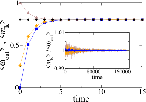
Figure 1: Time evolution of the conserved quantity $\omega_{\textrm{out}}$ (circles) and the densities of state-one nodes $m_{\bf k}$ in degree classes ${\bf k}=(k_{\textrm{in}},k_{\textrm{out}})=(2,1)$ (squares), $(4,3)$ (diamonds) and $(3,9)$ (triangles), for the voter model dynamics. Curves correspond to averages over $100$ realizations on a single random uncorrelated network with $N=10^{5}$ nodes, scale-free in-degree distribution with exponent $2.5$ and exponential out-degree distribution. While $\left<\omega_{\textrm{out}}\right>$ remains roughly constant over time, the densities quickly decay to the stationary value $\left<\omega_{\textrm{out}}\right>$. The inset shows that the ratio between the densities and the conserved quantity is close to one during the entire evolution.

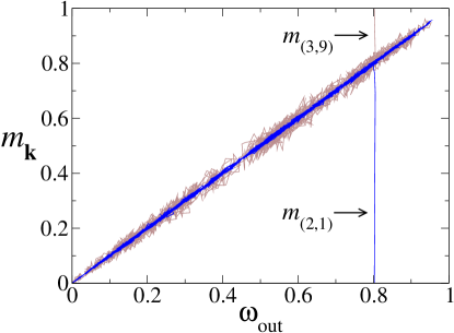
Figure 2: Densities of state-one nodes $m_{(2,1)}$ and $m_{(3,9)}$ vs $\omega_{\textrm{out}}$ in a single realization of the voter model dynamics on the same network of Fig. 1. The trajectories of classes $(2,1)$ and $(3,9)$ start at the positions $(0.8,0)$ and $(0.8,1.0)$ respectively, then they quickly hit and move along the diagonal $m_{\bf k}=\omega_{\textrm{out}}$, until they reach the zero-state consensus point $m_{(2,1)}=m_{(3,9)}=0$.

IV Voter model with link update

The same assumptions and procedures apply to the link-update voter model and the invasion process. The link update (LU) dynamics selects first a directed connection, so that the node at the tail will always transmit its state to the neighbor at the head.

The microscopic dynamics of the link-update voter model is described by

$$s_{u}(t+dt)=\mu_{u}(dt)\xi_{u}+(1-\mu_{u}(dt))s_{u}(t),$$ (21)

where as for the voter dynamics $\xi_{u}$ is given by Eq. (3) and the binary variable $\mu_{u}(dt)$ for the selection of a link has a probability distribution

$$P(\mu_{u}(dt))=k_{u,\textrm{in}}dt\delta_{\mu_{u}(dt),1}+(1-k_{u,\textrm{in}}dt)\delta_{\mu_{u}(dt),0}.$$ (22)

A factor $\lambda/(N\left<k_{\textrm{in}}\right>)$ has been reabsorbed in the definition of $dt$. Proceeding as for the voter model (we skip the details), we arrive to the equation for the evolution of the relative densities $m_{\bf k}$ for the different degree classes,

$$\frac{dm_{\bf k}(t)}{dt}=-k_{\textrm{in}}m_{\bf k}(t)+k_{\textrm{in}}\sum_{\bf k^{\prime}}P_{\textrm{in}}({\bf k^{\prime}}|{\bf k})m_{\bf k^{\prime}}(t).$$ (23)

Regarding the stationary state, the same result as for the voter model is found. The state-one relative densities behave again as $m_{\bf k}(t)=\sum_{\bf k^{\prime}}P_{\textrm{in}}({\bf k^{\prime}}|{\bf k})m_{\bf k^{\prime}}(t)$, so that all the relative densities are entangled through topological correlations. We can once again prove, within the heterogeneous mean field approach and for correlated strongly connected components, that a conserved quantity of the form $\omega=\sum_{\bf k}\varphi_{\bf k}m_{\bf k}(t)$ exists and is defined by the eigenvector problem

$$\tilde{\varphi}_{\bf k}=\sum_{\bf k^{\prime}}P_{\textrm{in}}({\bf k}|{\bf k^{\prime}})\tilde{\varphi}_{\bf k^{\prime}},$$ (24)

where now $\tilde{\varphi}_{\bf k}=k_{\textrm{in}}\varphi_{\bf k}$. In general, it is not possible to derive these coefficients without further specifying the form of degree-degree correlations in the network.

When two-point correlations are absent,

$$\frac{dm_{\bf k}(t)}{dt}=-k_{\textrm{in}}m_{\bf k}(t)+k_{\textrm{in}}\omega_{\textrm{out}}(t).$$ (25)

In the stationary state, $m_{\bf k}=\omega_{\textrm{out}}(t)\mbox{ }\forall{\bf k}$, but $\omega_{\textrm{out}}(t)$ is not a conserved quantity for the link update process as it was for the voter model. Instead, the conserved quantity is

$$\omega_{\textrm{oi}} = \left<\frac{k_{\textrm{out}}}{k_{\textrm{in}}}m_{\bf k}(t)\right>/\left<\frac{k_{\textrm{out}}}{k_{\textrm{in}}}\right>$$ (26)

$$= \sum_{\bf k}\frac{k_{\textrm{out}}}{k_{\textrm{in}}}P({\bf k})m_{\bf k}(t)/\langle\frac{k_{\textrm{out}}}{k_{\textrm{in}}}\rangle,$$

which follows from Eq. (25). Compare this expression with that for the total magnetization in uncorrelated undirected networks $w=\omega=\left(\sum_{k}P(k)m_{k}(t)\right)/\langle k\rangle$ which corresponds to the conserved quantity for those structures Suchecki et al. (2005b). The dependence of the conserved weighted magnetization on the ratio between out- and in-degree for directed networks highlights the fact that in LU it is important to have both a high out-degree to be influential and at the same time to have a low in-degree not to be too influenceable. Notice that the ratio of the directed degrees is well defined since we are assuming that the network is organized at the macroscopic scale into a SCC without peripheral components all nodes having at least one incoming and one outgoing link. Finally, in finite systems the probability of the state-one absorbing state is given by the conserved quantity, $\omega_{\textrm{oi}}=P_{1}$, and so fixed by the initial condition.

The derivation of how the state-one relative densities converge to their stationary value in uncorrelated networks is more intricate than for the voter model, but we can make use of a quasi-stationary approximation Gardiner (2004) in order to solve Eq. (25), exploiting the fact that $\omega_{\textrm{oi}}$ is the conserved quantity. In the stationary state $\omega_{\textrm{out}}=\omega_{\textrm{oi}}$, and we approximate the equation by

$$\frac{dm_{\bf k}(t)}{dt}=-k_{\textrm{in}}m_{\bf k}(t)+k_{\textrm{in}}\omega_{\textrm{oi}}.$$ (27)

For a given initial condition $m_{\bf k}(0)$, the solution is

$$m_{\bf k}(t)=\omega_{\textrm{oi}}(m_{\bf k}(0)-\omega_{\textrm{oi}})e^{-k_{\textrm{in}}t}.$$ (28)

As in the voter model, all the densities decay exponentially fast to the stationary value $\omega_{\textrm{oi}}$, but in contrast not all the densities decay with the same velocity, which depends on the in-degree. Higher in-degree classes have smaller relaxation times and decay faster than lower ones, but the transient is always faster as compared to the VM.

Table 1: Conserved quantities for voter-like models in strongly connected components of directed networks. 1st column, existence of conserved quantity for correlated networks; 2nd column, conserved quantity for uncorrelated networks; 3rd column, stationary values for the relative densities; 4th column, density decay.

	$\omega_{\textrm{corr}}$	$\omega_{\textrm{unc}}$	$m_{\bf k}^{st}$	$m_{\bf k}$
VM	$\exists$	$\omega_{\textrm{out}}=\frac{1}{\langle k_{\textrm{out}}\rangle}\sum_{\bf k}k_{\textrm{out}}P({\bf k})m_{\bf k}(t)$	$\omega_{\textrm{out}}$	$m_{\bf k}^{st}+(m_{\bf k}(0)-m_{\bf k}^{st})e^{-t}$
LU	$\exists$	$\omega_{\textrm{oi}}=\frac{1}{\langle k_{\textrm{out}}/k_{\textrm{in}}\rangle}\sum_{\bf k}k_{\textrm{out}}/k_{\textrm{in}}P({\bf k})m_{\bf k}(t)$	$\omega_{\textrm{oi}}$	$m_{\bf k}^{st}+(m_{\bf k}(0)-m_{\bf k}^{st})e^{-k_{\textrm{in}}t}$
IP	$\exists$	$\omega_{\textrm{in}}=\frac{1}{\langle 1/k_{\textrm{in}}\rangle}\sum_{\bf k}\frac{1}{k_{\textrm{in}}}P({\bf k})m_{\bf k}(t)$	$\omega_{\textrm{in}}$	$m_{\bf k}^{st}+(m_{\bf k}(0)-m_{\bf k}^{st})e^{-\frac{k_{\textrm{in}}}{\left<k_{\textrm{in}}\right>}t}$

V Invasion process

The invasion process (IP) picks nodes at random that export their state to a randomly chosen outgoing neighbor. A certain node $u$ will update its state in a passive form only when one of its incoming neighbors $v$ is selected as the first node in one iteration of the dynamics and then $v$ chooses $u$ among all its outgoing neighbors to transmit it its state. In this situation, it is more convenient to work with the probability of node $u$ undergoing a state update with final state 1, $\xi_{u}^{(1)}$, and the probability of node $u$ undergoing a state update with final state 0, $\xi_{u}^{(0)}$. The probability distributions of these dichotomic stochastic variables are

$$P(\xi_{u}^{(1)}) = \Phi_{u}^{1}dt\delta_{\xi_{u}^{(1)},1}+(1-\Phi_{u}^{1}dt)\delta_{\xi_{u}^{(1)},0},$$ (29)

$$P(\xi_{u}^{(0)}) = \Phi_{u}^{0}dt\delta_{\xi_{u}^{(0)},1}+(1-\Phi_{u}^{0}dt)\delta_{\xi_{u}^{(0)},0},$$ (30)

with

$$\Phi_{u}^{1}(t) = \sum_{v}a_{vu}s_{v}(t)/k_{v,\textrm{out}},$$ (31)

$$\Phi_{u}^{0}(t) = \sum_{v}a_{vu}(1-s_{v}(t))/k_{v,\textrm{out}}$$ (32)

and the parameter $\lambda$ of the Poisson process for the happening of events reabsorbed in $dt$. Using these expressions, the dynamics is described at the microscopic scale by

$$s_{u}(t+dt) = \xi_{u}^{(1)}(dt)(1-\xi_{u}^{(0)}(dt))$$ (33)

$$+ (1-\xi_{u}^{(1)}(dt))(1-\xi_{u}^{(0)}(dt))s_{u}(t).$$

Following the same methodology as for the voter model, the drift equations for the relative densities in the different degree classes read

$$\frac{dm_{\bf k}(t)}{dt}=k_{\textrm{in}}\sum_{\bf k^{\prime}}\frac{1}{k^{\prime}_{\textrm{out}}}P_{\textrm{in}}({\bf k^{\prime}}|{\bf k})(m_{\bf k^{\prime}}(t)-m_{\bf k}(t)).$$ (34)

The existence of a conserved quantity $\omega=\sum_{\bf k}\varphi_{\bf k}m_{\bf k}(t)$ in the correlated case is governed by the eigenvalue problem

$$\tilde{\varphi}_{\bf k}=\sum_{\bf k^{\prime}}\frac{P_{\textrm{in}}({\bf k}|{\bf k^{\prime}})/k_{\textrm{out}}}{\sum_{\bf k^{\prime\prime}}P_{\textrm{in}}({\bf k^{\prime\prime}}|{\bf k^{\prime}})/k_{\textrm{out}}^{\prime\prime}}\tilde{\varphi}_{\bf k^{\prime}},$$ (35)

where $\tilde{\varphi}_{\bf k}=\varphi_{\bf k}k_{\textrm{in}}\sum_{\bf k^{\prime\prime}}P_{\textrm{in}}({\bf k^{\prime\prime}}|{\bf k})/k_{\textrm{out}}^{\prime\prime}$. Summing both sides of this equation over ${\bf k}$, one arrives once more to a trivial identity and so a conserved quantity exists in general on networks with degree-degree correlations. As we see next, we can be more specific on uncorrelated networks, for which Eq. (34) reduces to

$$\frac{dm_{\bf k}(t)}{dt}=\frac{k_{\textrm{in}}}{\left<k_{\textrm{in}}\right>}(m(t)-m_{\bf k}(t)),$$ (36)

where $m(t)=\sum_{\bf k}P({\bf k})m_{\bf k}(t)$ is the total density of state-one nodes in the network.

In the stationary state, $m_{\bf k}(t)=m(t)\mbox{ }\forall{\bf k}$, but here $m(t)$ is not a conserved quantity for the IP in uncorrelated directed networks. Instead, the conserved quantity is

$$\omega_{\textrm{in}}(t) = \left<\frac{m_{\bf k}(t)}{k_{\textrm{in}}}\right>/\left<\frac{1}{k_{\textrm{in}}}\right>$$ (37)

$$= \sum_{\bf k}\frac{1}{k_{\textrm{in}}}P({\bf k})m_{\bf k}(t)/\left<\frac{1}{k_{\textrm{in}}}\right>.$$

In finite systems, the probability of the state-one absorbing state is given by this conserved quantity, $\omega_{\textrm{in}}=P_{1}$, and is therefore fixed by the initial condition. The dependence of the weights on the inverse of the in degree implies that those nodes with low in-degree, so less influenceable, have the highest contribution and control the process. This dependence on the in degree is analogous to the dependence on the degree of the conserved quantity $w=\omega=\left(\sum_{k}1/kP(k)m_{k}(t)\right)/\langle k\rangle$ in uncorrelated undirected networks Sood et al. (2008).

After a transient, $m(t)$ reaches the value $\omega_{\textrm{in}}$, so that the stationary values of the relative densities are $m_{\bf k}(t)=\omega_{\textrm{in}}\mbox{ }\forall{\bf k}$. This result tells us that all the densities become independent of ${\bf k}$ and reach the same stationary value, as in the previous processes.

The derivation of how the state-one relative densities converge to their stationary value in uncorrelated networks is more intricate than for the voter model, but like for the link update we can make use of a quasi-stationary approximation Gardiner (2004) in order to solve Eq. (36). Substituting into Eq. (36) that in the stationary state $m(t)=\omega_{\textrm{in}}$,

$$\frac{dm_{\bf k}(t)}{dt}=\frac{k_{\textrm{in}}}{\left<k_{\textrm{in}}\right>}\left(\omega_{\textrm{in}}-m_{\bf k}(t)\right).$$ (38)

For a given initial condition $m_{\bf k}(0)$, the solution is

$$m_{\bf k}(t)=\omega_{\textrm{in}}+\left(m_{\bf k}(0)-\omega_{\textrm{in}}\right)e^{-\frac{k_{\textrm{in}}}{\left<k_{\textrm{in}}\right>}t}.$$ (39)

All the densities decay exponentially to the stationary value $\omega_{\textrm{in}}$. Higher in-degree classes decay faster than lower ones with a relaxation time that is proportional to the inverse of the in-degree, as is the case for LU. Due to the average degree in the relaxation time, however, transients are generally slower in the IP than in the LU. When compared with the VM, the IP dynamics exhibits a slower transient for degree classes with in-degree below average while those with in-degree above the average converge faster to the stationary state.

VI Conclusions

We have introduced an analytical formalism from microscopic dynamics to show that three different nonequilibrium dynamical models with two-absorbing states running on strongly connected components of directed networks with heterogeneous degrees and degree-degree correlations have associated ensemble average conservation laws. These conservation laws have been fully determined when degree-degree correlations are absent. The existence of ensemble average conservation laws is a general characteristic of Markov processes with two or more absorbing states.

The constraints imposed on the dynamics by the conservation laws lead to interesting and nontrivial behavior. From a practical point of view, they are related to the stationary values and the characteristic relaxation times of the relative densities of nodes in state one in each degree class and, in finite systems, gives the probabilities of reaching the two possible absorbing states. In this sense, the conservation laws obtained in the thermodynamic limit for a system that does not order in that limit (i.e. does not reach the absorbing state) determine the probabilities of reaching each absorbing state for a finite system. The contribution of each node to he conserved global weighted magnetization is always a specific function of the directed degrees. In the case of the VM, the out-degree is the weight that controls the importance of the node as a measure of its influence, while in the IP it is the inverse of the in-degree, and in the LU it is the ratio between out and in-degree. In all cases, the conserved quantities are determined by local properties that encode the importance of each node in the network. Depending on the dynamics, what seems important from a local perspective is to be influential reaching a large number of neighbors, or not to be too influenceable, with a low number of incoming connections, or both at the same time.

From a broad perspective, these studies help in the understanding of how the rich structure of real systems affects the dynamical processes that run on top. However, many questions still remain unsolved. In which specific way do degree correlations alter the results for uncorrelated networks? How is the diffusive fluctuations regime in SCCs of finite directed networks? Is the finite size scaling of consensus times the same as in undirected networks? On the other hand, it seems realistic to restrict to SCCs for a number of densely connected systems, like for instance the world trade web Serrano et al. (2007), but in sparse directed networks the whole structure of core and peripheral components should be taken into account. Numerical simulations in some specific model networks Park and Kim (2006) show that the appearance of an input component seems to prevent the system, even if finite, from reaching an absorbing state for specific initial conditions. How does the complete structure of a directed network couples to the initial conditions of the dynamics to induce the presence of zealots and how do they affect in quantitative terms the behavior of the whole system still needs further research.

During the final completion of this work, we became aware of a recent preprint Masuda and Ohtsuki (2008) discussing the fixation probabilities of mutants for Voter-like dynamics on directed networks. Since there exists a direct relation between fixation probabilities of mutants and exit probabilities, and so conserved quantities, some of the results derived in that paper –without reference to conservation laws- concerning the dependence on the directed degrees are in correspondence to some of our results on uncorrelated strongly connected components.