Gravity Effects on Neutrino Masses in Split Supersymmetry

Abstract

The mass differences and mixing angles of neutrinos can neither be explained by R-Parity violating split supersymmetry nor by flavor blind quantum gravity alone. It is shown that combining both effects leads, within the allowed parameter range, to good agreement with the experimental results. The atmospheric mass is generated by supersymmetry through mixing between neutrinos and neutralinos, while the solar mass is generated by gravity through flavor blind dimension five operators. Maximal atmospheric mixing forces the tangent squared of the solar angle to be equal to $1/2$. The scale of the quantum gravity operator is predicted within a $5\%$ error, implying that the reduced Planck scale should lie around the GUT scale. In this way, the model is very predictive and can be tested at future experiments.

I Introduction

The existence of neutrino masses and mixing angles is experimentally well confirmed and therefore the theoretical understanding and description of those quantities is one of the most urgent issues for particle physics NeutrinoReview . There are two frequently studied theoretical extensions of the standard model of particle physics which also were expected to explain the origin and the shape of the small but non zero neutrino mass matrix.

On the one hand there is Supersymmetry. Although there is no experimental evidence for supersymmetry, it is often invoked that the unification of gauge coupling constants at the GUT scale is an indirect indication for supersymmetry. It has been pointed out that this gauge unification is achieved even if all scalar superpartners of quarks and leptons are very heavy, introducing the scenario called Split Supersymmetry (SS) SPLIT ; Bajc:2004hr . The original SS scenario includes R-Parity conservation, which guarantees the stability of the LSP and thus a Dark Matter candidate, and only one light Higgs doublet, which behaves like the SM Higgs. Despite the fact that models with R-Parity Violation (RpV) loose the LSP as a dark matter candidate, they are studied because they provide a compelling mechanism for the generation of neutrino masses Rparity-neutrinos . Nevertheless, SS models with RpV are incapable to produce the necessary neutrino masses, even in next to leading order calculations Chun:2004mu ; Diaz:2006ee ; Davidson:2000uc .

On the other hand there is the possible existence of non-renormalizable gravitational interactions. Those interactions could have an influence on the neutrino sector of the standard model Barbieri:1979hc ; Akhmedov:1992hh ; Akhmedov:1992et ; deGouvea:2000jp ; Dighe:2006sr ; Vissani:2003aj . Although the standard Planck scale $M_{P}=1.2\times 10^{19}$ GeV generates a solar mass which is too small to fit the experimental evidence, a lowered Planck scale $M_{f}$ might in principle do the job. However, gravitational interactions are expected to be “flavor blind” and it has been shown that therefore a purely gravitational neutrino sector is also incapable to explain the existence of three different neutrino masses Berezinsky:2004zb .

In this paper we study the combined effect of the supersymmetrical and gravitational neutrino sector. We find that the combination of both effects can explain all present neutrino data. But this kind of model even leads to predictions for the solar neutrino mixing angle $\sin^{2}\theta_{sol}$ and for the scale of the gravitational contribution.

II The neutrino mass matrix in R-parity violating SPLIT SUSY

In Split SUSY all scalars are very heavy, except for one Higgs doublet SPLIT . Since we are interested in the possibility to describe the neutrino masses in Split-SUSY, we need to consider R-Parity violating interactions Rparity . Knowing all relevant trilinear R-parity violating interactions one can calculate the neutralino/neutrino mass matrix. Integrating out the neutralinos from this matrix, one finds that the neutrino mass matrix in flavor space is given by Diaz:2006ee :

$${\bf M}_{\nu}^{eff}=\frac{v^{2}}{4\det{M_{\chi^{0}}}}\left(M_{1}\tilde{g}_{d}^{2}+M_{2}\tilde{g}^{\prime 2}_{d}\right)\left[\begin{array}[]{cccc}\lambda_{1}^{2}&\lambda_{1}\lambda_{2}&\lambda_{1}\lambda_{3}\cr\lambda_{2}\lambda_{1}&\lambda_{2}^{2}&\lambda_{2}\lambda_{3}\cr\lambda_{3}\lambda_{1}&\lambda_{3}\lambda_{2}&\lambda_{3}^{2}\end{array}\right]\quad,$$ (1)

where the determinant of the neutralino mass matrix is:

$$\det{M_{\chi^{0}}}=-\mu^{2}M_{1}M_{2}+\frac{1}{2}v^{2}\mu\left(M_{1}\tilde{g}_{u}\tilde{g}_{d}+M_{2}\tilde{g}^{\prime}_{u}\tilde{g}^{\prime}_{d}\right)+\textstyle{\frac{1}{16}}v^{4}\left(\tilde{g}^{\prime}_{u}\tilde{g}_{d}-\tilde{g}_{u}\tilde{g}^{\prime}_{d}\right)^{2}\quad.$$ (2)

Here, $v$ is the vacuum expectation value of the light Higgs field, $M_{1}$, $M_{2}$ are the gaugino masses. Further, $\tilde{g}_{u,d}$ and $\tilde{g}^{\prime}_{u,d}$ are the trilinear couplings between the Higgs boson, the gauginos, and the higgsinos. The parameters $\lambda_{i}\equiv a_{i}\mu+\epsilon_{i}$ Diaz:2006ee are related to the traditional BRpV parameters $\Lambda_{i}$ Nowakowski:1995dx by $\Lambda_{i}=\lambda_{i}v_{d}$. The $\epsilon_{i}$ are the parameters that mix higgsinos with leptons, and $a_{i}$ are dimensionless parameters that mix gauginos with leptons. Finally, $\mu$ is the higgsino mass.

This effective neutrino mass matrix ${\bf M}_{\nu}^{eff}$ has only one eigenvalue different from zero. As in the case of R-parity violation in the MSSM with bilinear terms, only one neutrino is massive. As it is explained in the literature Chun:2004mu ; Diaz:2006ee , in SS it is not possible to explain the neutrino masses and mixing using bilinear terms only. Further allowing for trilinear couplings makes it in principle possible to obtain solar neutrino masses and mixing. However this possibility was not discussed here, because it only works for a very special choice of parameters with an undesired hierarchical structure among the trilinear couplings Chun:2004mu . Without this hierarchical structure, the trilinear couplings become irrelevant because they contribute through loops of sparticles that have a mass of the order of the split supersymmetric scale $\widetilde{m}$, and therefore, decoupled.

III The neutrino mass matrix from low scale gravity effects

It is widely assumed that the unknown quantum gravity Lagrangian can be expanded to low energies. In flavor space this expansion can give rise to a non-renormalizable term in the Lagrangian of the type

$${\cal L}\sim\frac{\tilde{\lambda}_{ij}}{M_{P}}\overline{\psi}_{i}\psi_{j}\phi^{2}\quad.$$ (3)

Here, $\psi_{i}$ and $\phi$ are the lepton and Higgs fields respectively. In an idealized model the flavor mixing coefficients $\tilde{\lambda_{ij}}$ can all be taken to be of order one Barbieri:1979hc ; Akhmedov:1992hh ; Akhmedov:1992et ; deGouvea:2000jp ; Berezinsky:2004zb ; Dighe:2006sr . When the Higgs acquires a vacuum expectation value, a neutrino mass is generated

$$m_{\nu}\sim{\cal O}(1)\frac{v^{2}}{M_{P}}\sim{\cal O}(10^{-6})\,\,{\mathrm{eV}}\quad,$$ (4)

with $v$ the electroweak vacuum expectation value. This type of contribution to the neutrino mass matrix has also been explored in Joshipura:1998qn . Since this neutrino mass term is too small, we look into the possibility that the true Planck scale $M_{f}$ is actually much lower than $M_{P}$. Such a lowered Planck scale $M_{f}$ is an intrinsic prediction of models with compact extra dimensions. In some of those models the experimentally allowed Planck scale $M_{f}$ can be as low as one TeV Antoniadis:1998ig ; Randall:1999vf ; Randall:1999ee . However, a TeV gravity scale in operators like in eq. (3) meets strong constraints from precision measurements such as $\mu\rightarrow e\gamma$ Berezhiani:1998wt . This can be met by imposing additional symmetries or by admitting that $M_{f}$ might not be so extremely small

$$1\,{\mathrm{TeV}}\ll M_{f}<M_{P}\quad.$$ (5)

Several papers Barbieri:1979hc ; Akhmedov:1992hh ; Akhmedov:1992et ; deGouvea:2000jp ; Berezinsky:2004zb ; Dighe:2006sr discuss contributions of an exact “blindness” model, where the part of the neutrino mass matrix coming from gravitational effects can be parameterized in flavor space as

$$\Delta M_{g}^{\nu}=\mu_{g}\left[\begin{array}[]{cccc}1&1&1\cr 1&1&1\cr 1&1&1\end{array}\right]\quad,$$ (6)

where

$$\mu_{g}\sim{\cal O}(1)\frac{v^{2}}{M_{f}}\sim{\cal O}(10^{-2})\,\,{\mathrm{eV}}\quad.$$ (7)

It should be to noticed that such an exact “blindness” model does not imply base independence in flavor space. This means that only when written in the flavor base (defined by a diagonal mass matrix of the charged Leptons), the matrix (6) takes its symmetric form. Further, such a model can only give direct predictions for the UPMNS matrix (17) if the relation of flavor basis to the mass basis is defined for the charged leptons as well. Like in the standard model this relation is implicitly assumed for the above contribution by taking both basis to coincide Dighe:2006sr .

In order to explain the solar mass scale the fundamental scale has to be $M_{f}\sim{\cal O}(10^{15})\,\,{\mathrm{GeV}}$, which is in good agreement with the inequality in eq. (5). However, the matrix in eq. (6) has only one eigenvalue different from zero. Therefore such a scenario can not account for both solar and atmospheric neutrino mass splittings.

IV The neutrino mass matrix from R-parity violating SPLIT SUSY and low scale quantum gravity

Now we will discuss the possibility that both, R-parity violating Split Susy and low scale quantum gravity operators like eq. (3) contribute to the Lagrangian. In this case, two terms can contribute to the neutrino mass matrix. Since the mass terms in eqs. (1) and (6) are both formulated in flavor space one can write the total effective neutrino mass matrix as,

$$M_{g}^{\nu ij}=A\lambda^{i}\lambda^{j}+\mu_{g}\quad,$$ (8)

where we defined the factor in front of the mass matrix in equation (1) as $A$. As defined above, the neutrino mass matrix does not contain CP violating phases. In this case, if $A>0$ and $\mu_{g}>0$ the three neutrino masses are

$$m_{\nu_{1}} = 0$$

$$m_{\nu_{2}} = \frac{1}{2}\left(A|\vec{\lambda}|^{2}+3\mu_{g}\right)-\frac{1}{2}\sqrt{\left(A|\vec{\lambda}|^{2}+3\mu_{g}\right)^{2}-4A\mu_{g}|\vec{v}\times\vec{\lambda}|^{2}}$$ (9)

$$m_{\nu_{3}} = \frac{1}{2}\left(A|\vec{\lambda}|^{2}+3\mu_{g}\right)+\frac{1}{2}\sqrt{\left(A|\vec{\lambda}|^{2}+3\mu_{g}\right)^{2}-4A\mu_{g}|\vec{v}\times\vec{\lambda}|^{2}}$$

where we have defined the auxiliary vector $\vec{v}=(1,1,1)$. In the approximation where the $\mu_{g}$ term is subdominant, the squared mass differences are given by,

$$\Delta m^{2}_{sol} = (m_{2}^{2}-m_{1}^{2})=\mu_{g}^{2}\frac{(\vec{v}\times\vec{\lambda})^{4}}{\vec{\lambda}^{4}}+{\mathcal{O}}(\mu_{g}^{3})$$ (10)

$$\Delta m^{2}_{atm} = (m_{3}^{2}-m_{2}^{2})=A\vec{\lambda}^{4}+2A\mu_{g}(\vec{v}\vec{\lambda})^{2}+{\mathcal{O}}(\mu_{g}^{3})$$ (11)

This shows that for a very small $\mu_{g}$, the atmospheric mass scale is controlled by the parameter $A$ and the solar mass scale is controlled by $\mu_{g}$. In this approximation, the eigenvectors are equal to,

$$\vec{v}_{1} = \frac{\vec{v}\times\vec{\lambda}}{|\vec{v}\times\vec{\lambda}|}$$

$$\vec{v}_{2} = \frac{\vec{\lambda}\times(\vec{v}\times\vec{\lambda})}{|\vec{\lambda}\times(\vec{v}\times\vec{\lambda})|}+{\cal O}(\mu_{g})$$ (12)

$$\vec{v}_{3} = \frac{\vec{\lambda}}{|\vec{\lambda}|}+{\cal O}(\mu_{g})$$

and the matrix $U_{PMNS}$ is formed with the eigenvectors in its columns. The neutrino mixing matrix is defined as

$$U_{PMNS}=U_{32}U_{31}U_{21}\quad,$$ (13)

where $U_{32}$ is a rotation matrix around the axis one (with cyclic permutations for the other two).

At this point it is instructive to have a closer look at the matrix $U_{PMNS}$. This matrix appears in the Lagrangian of the leptonic charged current interactions such that,

$${\cal L}\owns-\frac{g}{\sqrt{2}}\big{(}\bar{e}_{L}^{+},\bar{\mu}_{L}^{+},\bar{\tau}_{L}^{+}\big{)}W_{\mu}^{-}\gamma^{\mu}U_{PMNS}\left(\begin{matrix}\nu_{1}\cr\nu_{2}\cr\nu_{3}\end{matrix}\right)$$ (14)

where fermions are in the mass eigenstate basis. In the most general situation, both the charged lepton and neutrino mass matrices are non-diagonal in the interaction basis,

$${\cal L}\owns-\big{(}\bar{e}^{\prime+}_{L},\bar{\mu}^{\prime+}_{L},\bar{\tau}^{\prime+}_{L}\big{)}M_{\ell}\left(\begin{matrix}e^{\prime-}_{L}\cr\mu^{\prime-}_{L}\cr\tau^{\prime-}_{L}\end{matrix}\right)-\big{(}\bar{\nu}^{\prime c}_{1},\bar{\nu}^{\prime c}_{2},\bar{\nu}^{\prime c}_{3}\big{)}M_{\nu}\left(\begin{matrix}\nu^{\prime}_{1}\cr\nu^{\prime}_{2}\cr\nu^{\prime}_{3}\end{matrix}\right)$$ (15)

where the prime on the fermion fields denote the interaction basis. The two mass matrices are diagonalized by $V_{\ell}$ and $V_{\nu}$,

$$V_{\ell}^{\dagger}M_{\ell}V_{\ell}={\mathrm{diag}}(m_{e},m_{\mu},m_{\tau})\,,\qquad V_{\nu}^{\dagger}M_{\nu}V_{\nu}={\mathrm{diag}}(m_{\nu_{1}},m_{\nu_{2}},m_{\nu_{3}})$$ (16)

and the $U_{PMNS}$ matrix becomes,

$$U_{PMNS}=V_{\ell}^{\dagger}V_{\nu},$$ (17)

where we have assumed CP conservation. Due to the Majorana nature of neutrinos, $U_{PMNS}$ depends on three mixing angles and three Majorana phases. We assume the latter to be zero. In general, a simultaneous diagonalization of $M_{\nu}$ and $M_{\ell}$ is necessary to find $U_{PMNS}$. In principle there might be also off-diagonal contributions to the matrix $M_{\ell}$ coming from the “flavor blind” gravitational terms in eq. (3) (R-parity violating supersymmetric intercations do not modify $V_{\ell}$). However, those contributions (if they are present) can be depreciated in our model since they only can produce corrections to the diagonal mass matrix of the charged leptons of the order $\mu_{g}/m_{e}\sim 10^{-8}$. This makes $V_{\ell}$ equal to unity up to terms of the order of $\mu_{g}/m_{e}$. In order to have a predictive model we do not consider any other beyond the standard model contributions, like non-diagonal terms in the Yukawa couplings of the charged leptons. Therefore, one can identify $U_{PMNS}$ with $V_{\nu}$. It is in this basis that we include the “flavor blind” contribution from gravity given in eq. (6).

V Results and Predictions

In this section we present some numerical results, where we find eigenvalues and eigenvectors of the $3\times 3$ effective neutrino mass matrix using numerical methods. With them, we find neutrino mass differences and mixing angles, and compare them with values from experimental measurements. The solar and atmospheric mass differences, as well as the solar and atmospheric mixing angles, have been measured in several experiments.

Table 1: Experimental measurements for neutrino parameters

Observable $o_{i}$	Mean value $\bar{o}_{i}$	$3\sigma_{i}$ variance	Units
$\Delta m_{atm}^{2}$	$2.35\times 10^{-3}$	$0.95\times 10^{-3}$	eV2
$\Delta m_{sol}^{2}$	$8.15\times 10^{-5}$	$0.95\times 10^{-5}$	eV2
$\sin^{2}\theta_{atm}$	$0.51$	$0.17$	-
$\sin^{2}\theta_{sol}$	$0.305$	$0.075$	-

We use the results of the combined analysis in ref. Maltoni:2004ei , given in Table I.

Table 2: Experimental upper bounds for neutrino parameters

Observable $o_{i}$	$3\sigma_{i}$ upper bound	Units
$\sin^{2}\theta_{reac}$	$0.047$	-
$m_{\beta\beta}$	$0.84$	eV

In addition, upper bounds have been obtained for the reactor angle Maltoni:2004ei , and for the neutrino less double beta decay mass parameter $m_{\beta\beta}$. The value for the neutrino less double beta decay parameter is quite precisely determined in our setting. Our model allows values of $0.001$ eV$<m_{\beta\beta}<0.005$ eV which is two orders of magnitude below the current experimental bound.

We scan the parameters space, varying randomly the parameters $\lambda_{i}$, $A$, and $\mu_{g}$, and calculate the goodness of the model, represented by eq. (8), with

$$\chi^{2}=\sum_{i}^{6}\frac{(o_{i}-\bar{o}_{i})^{2}}{(3\sigma_{i})^{2}}\quad.$$ (18)

where we have assigned a null mean value to the two parameters in Table II for which only upper bounds are known. Positive and negative solutions for $A$ were found. A typical solution for negative $A$ is

$$\lambda_{1}=0.0148\,{\mathrm{GeV}^{2}}\,,\quad\lambda_{2}=0.0822\,{\mathrm{GeV}^{2}}\,, \lambda_{3}=-0.0712\,{\mathrm{GeV}^{2}}\,,$$ (19)

$$A=-4.10\,{\mathrm{eV}}/{\mathrm{GeV}}^{4}\,, \mu_{g}=0.003\,{\mathrm{eV}}$$ (20)

with $\chi^{2}=0.02$. This shows that it is possible to find solutions for the combined model which are in ($3\sigma$) agreement with every single neutrino observable.

Table 3: Predictions for neutrino parameters

Observable	Value	Units
$\Delta m_{atm}^{2}$	$2.39\times 10^{-3}$	eV2
$\Delta m_{sol}^{2}$	$7.74\times 10^{-5}$	eV2
$\sin^{2}\theta_{atm}$	$0.596$	-
$\sin^{2}\theta_{sol}$	$0.321$	-
$\sin^{2}\theta_{reac}$	$0.023$	-
$m_{\beta\beta}$	$0.0039$	eV

The prediction for the neutrino parameters in this case are summarized in Table III.

Based on the same $3\sigma$-limits scan, we study how the parameters of this model are constrained by the experimental data. A key ingredient of this model is that it offers a possible way to measure $\mu_{g}$ for “flavor blind” gravity effects. Indeed, an interesting prediction is that the allowed values of the mass parameter $\mu_{g}$ are strongly constrained.

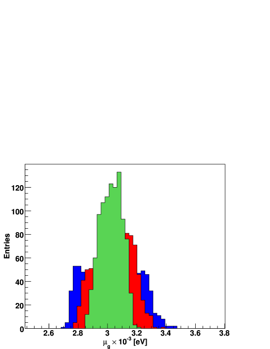
Figure 1: Prediction for the mass parameter $\mu_{g}$ among models that satisfy all the experimental constraints.

In Fig. 1 we show the frequency of occurrence of each value of $\mu_{g}$ among the selected models. This model predicts values centered around $\mu_{g}=3\times 10^{-3}$ eV with a 5% error, as we can see from the green region defined by $\chi^{2}<1$. For comparison we show also the red region for $\chi^{2}<2$, and the blue region for $\chi^{2}<3$. According to eq. (7), this implies a prediction for the true Planck scale given by $M_{f}\approx 2\times 10^{16}$ GeV, which is remarkably similar to the GUT scale.

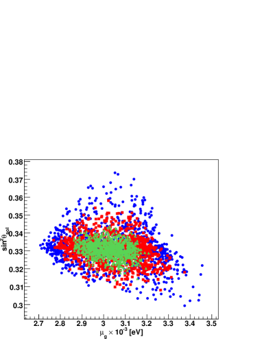
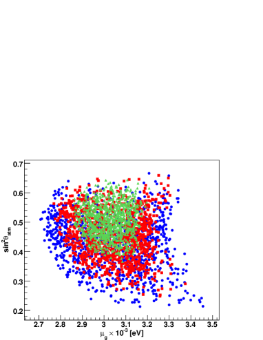
Figure 2: Sections of the parameter space showing $\sin^{2}\theta_{sol}$ and $\sin^{2}\theta_{atm}$ as a function of $\mu_{g}$, with $\chi^{2}<1,2,3,$ for green triangles, red squares, and blue circles respectively.

The same scan is shown in Fig. 2 where we see the neutrino mixing angles in correlation with the gravitational neutrino mass parameter $\mu_{g}$. Concentrating on the green triangles ($\chi^{2}<1$), we see that the values of $\sin^{2}\theta_{sol}$ (left frame) are centered around 0.33, which is in the larger side of the experimentally allowed window. On the other hand, the values of $\sin^{2}\theta_{atm}$ are centered around one half, which is right in the center of the experimental window. For comparison we show also points of parameter space less favored by experimental data, with red squares corresponding to $\chi^{2}<2$, and blue circles to $\chi^{2}<3$.

Since the reactor angle satisfy,

$$\sin^{2}\theta_{reac}=(v_{3,1})^{2}=\frac{\lambda_{1}^{2}}{|\vec{\lambda}|^{2}}<0.047$$ (21)

where $v_{3,1}$ is the first component of the third eigenvector in eq. (12), and the quoted upper bound corresponds to the one given in Table II, we need $\lambda_{1}^{2}\ll\lambda_{2}^{2}+\lambda_{3}^{2}$. Neglecting the value of $\lambda_{1}$ in front of $\lambda_{2}$ and $\lambda_{3}$ we obtain,

$$\tan^{2}\theta_{atm} = \left(\frac{v_{3,2}}{v_{3,3}}\right)^{2}=\frac{\lambda_{3}^{2}}{\lambda_{2}^{2}}=1$$

$$\tan^{2}\theta_{sol} = \left(\frac{v_{2,1}}{v_{3,1}}\right)^{2}=\frac{\lambda_{2}^{2}+\lambda_{3}^{2}}{(\lambda_{3}-\lambda_{2})^{2}}=\frac{1}{2}$$ (22)

The numerical values for each parameter shown in eq. (22) are obtained in the following scenario. Experimental results indicate $\sin^{2}\theta_{atm}=0.51\pm 0.17$, where again we indicate the $3\sigma$ error. Maximal mixing is satisfied if we take $\lambda_{3}^{2}=\lambda_{2}^{2}$. Choosing the sign $\lambda_{3}=-\lambda_{2}$ leads to the prediction for the solar angle indicated in the previous equation, $\sin^{2}\theta_{sol}=1/3$, which nicely agrees with the experimental result $\sin^{2}\theta_{sol}=0.305\pm 0.075$.

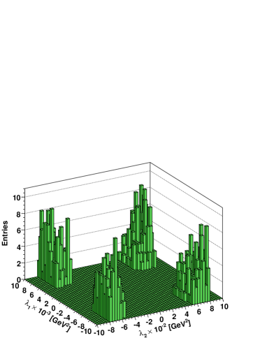
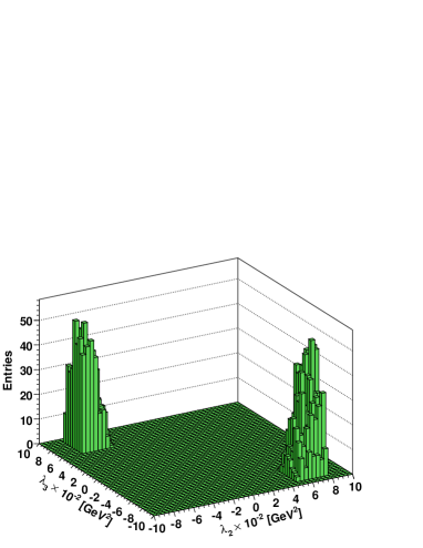
Figure 3: Frequency of occurrence for the parameters $\lambda_{i}$ among the models compatible with experimental results.

As we will see now, this prediction is confirmed by the scan and the numerical diagonalization of the neutrino mass matrix. In Fig. 3 we plot the frequency of occurrence for each of the parameters $\lambda_{i}$ among the models in our scan which satisfy the experimental constraints detailed in Tables I and II. We see in the left frame that $\lambda_{1}$ is typically an order of magnitude smaller than the other two parameters $\lambda_{2}$ and $\lambda_{3}$, consistent with requirements from the reactor angle. Due to this hierarchy in the parameters, our model has some interesting common features with the tri-bi-maximal mixing model discussed in Dighe:2006sr . In the right frame we see that models consistent with experiments need $\lambda_{3}=-\lambda_{2}$, leading to the prediction $\sin^{2}\theta_{sol}=1/3$ as explained earlier.

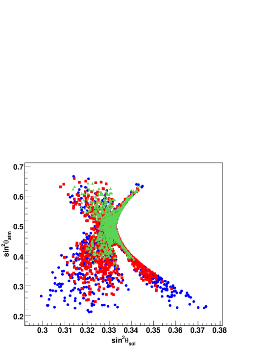
Figure 4: Section of the parameter space showing $\sin^{2}\theta_{atm}$ versus $\sin^{2}\theta_{sol}$, with $\chi^{2}<1,2,3$ for green triangles, red squares, and blue circles respectively.

The prediction $\tan^{2}\theta_{23}=1\Rightarrow\tan^{2}\theta_{sol}=1/2$, is observed also in our scan. In Fig. 4 the relation between the neutrino mixing parameters $\sin^{2}\theta_{atm}$ and $\sin^{2}\theta_{sol}$ is shown. From this plot one sees that the model can only deliver a good agreement with all experimental bounds, if $0.313<\sin^{2}\theta_{sol}<0.342$. This very strong constraint on $\sin^{2}\theta_{sol}$ (remember that the experimentally allowed region is $0.23<\sin^{2}\theta_{sol}<0.38$) gets even smaller if the atmospheric mixing parameter $\sin^{2}\theta_{atm}$ is taken at its central value of $0.51$, as seen in Fig. 4. In this case one finds that the model predicts $0.325<\sin^{2}\theta_{sol}<0.334$. With those small theoretical uncertainties an improved measurement of $\sin^{2}\theta_{sol}$ would already allow to confirm the model prediction or otherwise rule out this model.

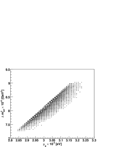
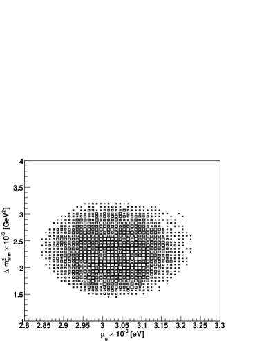
Figure 5: Sections of the parameter space showing $\Delta m^{2}_{sol}$ and $\Delta m^{2}_{atm}$ as a function of $\mu_{g}$ with $\chi^{2}<1$.

The neutrino mass differences $\Delta m^{2}_{sol}$ and $\Delta m^{2}_{atm}$ are shown in Fig. 5. The left frame shows that a growing $\mu_{g}$ gives a growing $\Delta m^{2}_{sol}$, which can be understood by comparing to the approximation in eq. (10), that is, the $A$ term dominates over the $\mu_{g}$ term in eq. (8). In the right frame we have the atmospheric mass difference $\Delta m^{2}_{atm}$ as a function of the gravitational neutrino mass parameter $\mu_{g}$, where there is no obvious dependence because the atmospheric mass difference is dominated by the $A$ term. In both mass differences though, we see that the predictions lie nicely at the center of the experimental window.

It is also instructive to study how the scale of the supersymmetric term $A$ and the scale of the gravitational term $\mu_{g}$ are pinned down by the individual experimental constraints in Table I. Starting from the benchmark point in eq. (19) and varying with respect to $A$ and $\mu_{g}$ we plot the allowed regions for every observable and the intersection of those regions.

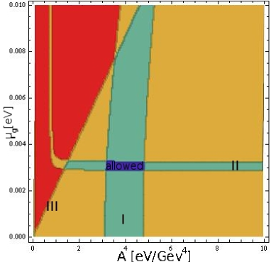
Figure 6: Allowed regions in the positive $A$-$\mu_{g}$ plane.

At the center of Fig. 6 we have the zone in the $A$-$\mu_{g}$ plane which is consistent with experiments, and formed by the intersection of several regions. Region I is a vertical stripe where mainly the $A$ parameter is constrained by the $\Delta m_{atm}^{2}$ data. Region II is a horizontal stripe where $\mu_{g}$ is constrained by the $\Delta m_{sol}^{2}$ data. Note that this horizontal stripe turns into a vertical one after an eigenvalue crossing, although this last branch is not allowed by the solar angle data. Finally, region III indicates the constraint from $\sin^{2}\theta_{sol}$, whose allowed region is at the right of the diagonal line, which breaks at the top also due to an eigenvalue crossing. Constraints from the other neutrino observables are not relevant for this figure.

The main features from Fig. 6 can be understood by looking at the approximations in eqs. (10) and (11), which show that for small values of $\mu_{g}$, the atmospheric mass difference $\Delta m_{atm}^{2}$ is dominated by $A$, while the solar mass difference $\Delta m_{sol}^{2}$ is dominated by $\mu_{g}$. One sees that in the vicinity of this benchmark point, the other observables play a minor role in pinning down the scale parameters $A$ and $\mu_{g}$.

VI Summary

It is known that in Split Supersymmetry with R-Parity violation an atmospheric mass difference is generated at tree level, but one-loop contributions are not enough to lift the symmetry of the effective neutrino mass matrix, thus not being able to generate a solar mass difference. This problem is not solved by adding the, in principle always present, “flavor blind” couplings from dimension five operators. The reason is that the Planck scale is too large to generate a solar mass difference large enough to be compatible with experiments. In this article we have shown that Split Supersymmetry with R-Parity violation, plus “flavor blind” gravity effects with a reduced Planck scale, present in models with compact extra dimensions, can be compatible with all data form neutrino experiments. The atmospheric mass difference is generated by supersymmetry with a mixing between neutrinos and neutralinos, while the solar mass difference is generated by the “flavor blind” gravitational effects. This model predicts a value for the gravitational term $\mu_{g}=3\times 10^{-3}\pm 5\%$ eV, which corresponds to a reduced Planck scale $M_{f}\approx 2\times 10^{16}$ GeV. The fact that this reduced Planck scale is equal to GUT scale is a tantalizing result that may be related to gauge coupling unification of all four forces. In addition, the solar mixing angle is predicted to satisfy $0.313<\sin^{2}\theta_{sol}<0.342$. We show also that a maximal atmospheric mixing $\sin^{2}\theta_{atm}=1/2$ implies $\sin^{2}\theta_{sol}=1/3$, which agrees with the implications from our parameter scan $0.325<\sin^{2}\theta_{sol}<0.334$, when we adopt the central value $\sin^{2}\theta_{atm}=0.51$. In this way, the model not only reproduce the experimental results but it is also predictive and, therefore, can be falsified by future experiments.