Ponderomotive acceleration of hot electrons in tenuous plasmas

Abstract

The oscillation-center Hamiltonian is derived for a relativistic electron injected with an arbitrary momentum in a linearly polarized laser pulse propagating in tenuous plasma, assuming that the pulse length is smaller than the plasma wavelength. For hot electrons generated at collisions with ions under intense laser drive, multiple regimes of ponderomotive acceleration are identified and the laser dispersion is shown to affect the process at plasma densities down to $10^{17}\,\text{cm}^{-3}$. Assuming $a/\gamma_{g}\ll 1$, which prevents net acceleration of the cold plasma, it is also shown that the normalized energy $\gamma$ of hot electrons accelerated from the initial energy $\gamma_{0}\lesssim\Gamma$ does not exceed $\Gamma\sim a\gamma_{g}$, where $a$ is the normalized laser field, and $\gamma_{g}$ is the group velocity Lorentz factor. Yet $\gamma\sim\Gamma$ is attained within a wide range of initial conditions; hence a cutoff in the hot electron distribution is predicted.

I Introduction

The recent advances in the laser technology have yielded techniques for generating electromagnetic radiation with intensities as high as $10^{22}\,\text{W}/\text{cm}^{2}$ ref:mourou06 . Experiments show that interaction of ultrapowerful pulses with underdense plasmas produce hot electrons with energies up to hundreds of MeV ref:mangles05 ; ref:chen99 . As argued in LABEL:ref:balakin06, the effect might be due to ponderomotive acceleration of electrons, following large-angle collisions with ions in strong electromagnetic field. Assuming that the laser dispersion is negligible due to the plasma density being small, the model explains the observed power-law spectra and predicts that the particle maximum energy scales as the third power of the field amplitude. This estimate is also in approximate agreement with the available experimental data ref:balakin06 ; however, the latter is insufficient to conclude whether the model is, in fact, quantitatively accurate. On the other hand, already small yet nonvanishing densities of the plasma can undermine the assumption of negligible dispersion and therefore modify the acceleration mechanism: the electron velocity can then exceed the group velocity of a laser pulse, so the particles can be reflected, or “snow-plowed” by the field envelope. Thus, to understand the production of hot electrons in previous and future experiments, the effect of the laser dispersion on ponderomotive acceleration must be explored.

Previously, the snow-plow acceleration was studied in specific regimes when the electron motion becomes exactly integrable. Particularly, Refs. ref:eloy06 ; ref:mendonca07 ; ref:mendonca09 assume equal group and phase velocities of the laser, and Refs. ref:mckinstrie96 ; ref:mckinstrie97 ; ref:du00 ; ref:startsev03 suppose circular polarization and cold electrons (i.e., having zero transverse momentum), also adopted in Refs. ref:ginzburg82 ; ref:ginzburg87 ; ref:rax92 ; ref:tokman99 for an oscillation-center model. However a general treatment of the relativistic ponderomotive force in plasma has not been formulated, and the effect of the laser dispersion on the ponderomotive acceleration of hot particles has not been understood.

The focus of this paper is then twofold. First, we derive the oscillation-center (OC) Hamiltonian for a relativistic electron injected with an arbitrary momentum in a linearly polarized laser pulse propagating in tenuous plasma, assuming that the pulse length $L_{{\scriptscriptstyle|{\kern-1.0pt}|}}$ is smaller than the plasma wavelength $\lambda_{p}$. Second, we use this formalism to describe the ponderomotive acceleration of hot electrons generated at collisions with ions under intense laser drive. Specifically, we identify multiple regimes of this acceleration and show that the laser dispersion affects the process at plasma densities down to $n\sim 10^{17}\,\text{cm}^{-3}$. Assuming $a/\gamma_{g}\ll 1$, which prevents net acceleration of the cold plasma, we also show that the normalized energy $\gamma$ of hot electrons accelerated from the initial energy $\gamma_{0}\lesssim\Gamma$ does not exceed $\Gamma\sim a\gamma_{g}$, where $a$ is the normalized laser field, and $\gamma_{g}$ is the group velocity Lorentz factor. Simultaneously, $\gamma\sim\Gamma$ is attained in a wide range of initial conditions, with the angular spread of the accelerated electrons $\chi\sim\gamma_{g}^{-1}$.

Hence we conclude that the distribution of hot electrons produced at large-angle collisions with ions at $L_{{\scriptscriptstyle|{\kern-1.0pt}|}}\ll\lambda_{p}$ and $a/\gamma_{g}\ll 1$ must have a cutoff at the energy $\gamma\sim a\gamma_{g}$. This refines the result from LABEL:ref:balakin06, showing how even weak laser dispersion can affect the acceleration gain. However, further experiments are yet needed to validate the updated scaling, because no relevant data has been reported for the regime considered here.

The paper is organized as follows. In Sec. II we introduce our basic equations. In Sec. III we derive the OC Hamiltonian for a particle interacting with a laser pulse in tenuous plasma. In Sec. IV we identify the major regimes of ponderomotive acceleration in plasma and find the general expression for the particle energy gain. In Sec. V, we discuss what we call the plateau regime, where $\gamma\sim\Gamma$ is attained within a wide range of initial conditions. In Sec. VI we summarize our main results. Supplementary calculations are given in Appendix.

II Basic equations

Suppose a plane laser wave propagating in plasma with the group velocity $v_{g{\kern 0.3pt}}$ and the phase velocity $v_{p{\kern 0.3pt}}$ along the $x$ axis, so the vector potential reads ${\boldsymbol{\rm A}}={\boldsymbol{\rm y}}^{0}{\kern-0.5pt}A$,

$$A=\mathcal{A}{\kern-1.0pt}\left(\frac{x-v_{g{\kern 0.3pt}}t}{L_{{\scriptscriptstyle|{\kern-1.0pt}|}}}\right){\kern-2.5pt}\cos(k[x-v_{p{\kern 0.3pt}}t]).$$ (1)

Here ${\boldsymbol{\rm y}}^{0}$ is a unit vector along the $y$ axis, $L_{{\scriptscriptstyle|{\kern-1.0pt}|}}$ is the spatial scale of the envelope $\mathcal{A}$, and $k$ is the wavenumber such that $\epsilon\equiv(kL_{{\scriptscriptstyle|{\kern-1.0pt}|}})^{-1}\ll 1$. Consider a particle with mass $m$ and charge $e$ interacting with this wave, assuming that the electrostatic potential is negligible (Sec. V.2). Then the particle Hamiltonian is book:landau2

$$H=c\sqrt{m^{2}c^{2}+p_{x}^{{\kern 0.7pt}2}+\left({\boldsymbol{\rm P}}_{\perp}-\frac{e}{c}\,{\boldsymbol{\rm A}}\right)^{\!2}},$$ (2)

where $p_{x}$ is the $x$ component of the particle kinetic momentum, and ${\boldsymbol{\rm P}}_{\perp}$ is the conserved transverse canonical momentum.

In the extended phase space, where $(t,-H)$ serves as another canonical pair and the independent variable is the proper time $\tau$, the equivalent Hamiltonian reads my:alfven

$$\mathfrak{H}=\frac{1}{2m}\,\Bigg{[}m^{2}c^{2}+p_{x}^{{\kern 0.7pt}2}+\left(P_{y}-\frac{e}{c}\,A\right)^{\!2}+P_{z}^{2}-\frac{H^{2}}{c^{2}}\Bigg{]},$$ (3)

and, numerically, ${\mathfrak{H}\equiv 0}$. Introduce the dimensionless variables

$$\bar{x}=kx,\qquad \rho=p_{x}/mc,$$ (4a)

$$\bar{t}=ckt,\qquad \gamma=H/mc^{2},$$ (4b)

$$\bar{\tau}=kc\tau,\qquad h=\mathfrak{H}/mc^{2},$$ (4c)

$$\beta_{g{\kern 0.3pt}}=v_{g{\kern 0.3pt}}/c,\qquad \beta_{p{\kern 0.3pt}}=v_{p{\kern 0.3pt}}/c,$$ (4d)

and ${\boldsymbol{\rm\mathscr{P}}}_{\perp}\equiv{\boldsymbol{\rm P}}_{\perp}/mc=\text{const}$. Hence we rewrite Eq. (3) as

$$h=\frac{1}{2}\,\Big{[}1+\rho^{2}+(\mathscr{P}_{y}-\bar{A})^{2}+\mathscr{P}_{z}^{2}-\gamma^{2}\Big{]},$$ (5)

assuming $\bar{\tau}$ is the new time, and the normalized laser field $\bar{A}\equiv eA/mc^{2}$ reads

$$\bar{A}=a\big{(}\epsilon{\kern 0.5pt}[{\kern 1.0pt}\bar{x}-\beta_{g{\kern 0.3pt}}\bar{t}{\kern 1.0pt}]\big{)}\cos(\bar{x}-\beta_{p{\kern 0.3pt}}\bar{t}).$$ (6)

III Oscillation-center Hamiltonian

III.1 Extended Hamiltonian

Like in Refs. ref:eloy06 ; ref:mendonca07 ; ref:mendonca09 ; ref:mckinstrie96 ; ref:mckinstrie97 ; ref:du00 ; ref:ginzburg82 ; ref:ginzburg87 ; ref:tokman99 , we assume the linear plasma dispersion, which holds for arbitrarily large $a$ at $L_{{\scriptscriptstyle|{\kern-1.0pt}|}}\ll\lambda_{p}$ ref:decker95 ; ref:sprangle90 ; foot:ed . [Also, the nonlinear instabilities will be neglected as they occur on time scales exceeding the acceleration time, which is less than the wave period (Sec. IV.2).] Then,

$$\beta_{g{\kern 0.3pt}}=\sqrt{1-\alpha},\quad\beta_{p{\kern 0.3pt}}=1/\sqrt{1-\alpha},$$ (7)

where $\alpha=n/n_{c}$, and $n_{c}$ is the critical density foot:waveguide .

Perform a canonical transformation on Eq. (5) foot:intact :

$$(\bar{x},\rho;\,\bar{t},-\gamma)\to(\theta,\mathcal{P};\,\psi,\mathcal{W}),$$ (8)

governed by the generating function

$$\mathcal{F}=(\bar{x}-\beta_{p{\kern 0.3pt}}\bar{t})\mathcal{P}+(\bar{x}-\beta_{g{\kern 0.3pt}}\bar{t})\mathcal{W}.$$ (9)

Then

$$\rho=\mathcal{P}+\mathcal{W},\quad\gamma=\beta_{p{\kern 0.3pt}}\mathcal{P}+\beta_{g{\kern 0.3pt}}\mathcal{W},$$ (10)

so the new Hamiltonian reads

$$\mathcal{H}=\frac{1}{2}\,\Bigg{\{}1-\frac{\alpha\mathcal{P}^{2}}{1-\alpha}+\alpha\mathcal{W}^{2}+\mathscr{P}_{z}^{2}+\\ +\big{[}\mathscr{P}_{y}-a(\epsilon\psi)\,\cos\theta\big{]}^{2}\Bigg{\}},$$ (11)

and the new variables are given by

$$\theta=\bar{x}-\beta_{p{\kern 0.3pt}}\bar{t},\quad\mathcal{P}=\frac{\gamma-\beta_{g{\kern 0.3pt}}\rho}{\beta_{p{\kern 0.3pt}}-\beta_{g{\kern 0.3pt}}},$$ (12)

$$\psi=\bar{x}-\beta_{g{\kern 0.3pt}}\bar{t},\quad\mathcal{W}=-\frac{\gamma-\beta_{p{\kern 0.3pt}}\rho}{\beta_{p{\kern 0.3pt}}-\beta_{g{\kern 0.3pt}}}.$$ (13)

Unlike at $\beta_{p{\kern 0.3pt}}=\beta_{g{\kern 0.3pt}}$ ref:eloy06 ; ref:mendonca07 ; ref:mendonca09 , e.g., for vacuum (Appendix A), or the exactly integrable case of circular polarization with zero $\mathscr{P}_{y}$ ref:mckinstrie96 ; ref:mckinstrie97 ; ref:du00 ; ref:startsev03 , there are two independent coordinates $\theta$ and $\psi$ entering $\mathcal{H}$ here; hence we proceed as follows. Introduce the normalized momenta

$$\bar{\mathcal{P}}=\alpha\mathcal{P},\quad\bar{\mathcal{W}}=\alpha\mathcal{W},$$ (14)

which remain finite at $\alpha\to 0$; hence the Hamiltonian

$$\bar{\mathcal{H}}=\frac{1}{2}\,\Bigg{\{}\alpha-\frac{\bar{\mathcal{P}}^{2}}{1-\alpha}+\bar{\mathcal{W}}^{2}+\alpha\mathscr{P}_{z}^{2}+\\ +\alpha\big{[}\mathscr{P}_{y}-a(\epsilon\psi)\,\cos\theta\big{]}^{2}\Bigg{\}}.$$ (15)

Following the general perturbation theory book:arnold ; ref:dewar73 ; ref:johnston78 ; ref:johnston79 , we now seek to map out the quiver dynamics. To do this, consider a canonical transformation

$$(\theta,\bar{\mathcal{P}};\,\psi,\bar{\mathcal{W}})\to(\Theta,{\kern-0.5pt}\slPi;\,\Psi,W)$$ (16)

governed by the generating function

$$F=\theta{\kern-0.5pt}\slPi+\psi W+S(\theta,{\kern-0.5pt}\slPi;\psi,W).$$ (17)

Choose $S$ such that ${\kern-0.5pt}\slPi$ and $W$ are OC canonical momenta, i.e., the new Hamiltonian $\mathrm{H}(\Theta,{\kern-0.5pt}\slPi;\Psi,W)$ does not contain fast oscillations. Then

$$\Bigg{\{}-\frac{1}{1-\alpha}\Big{[}2{\kern-0.5pt}\slPi\,\partial_{\theta}S+(\partial_{\theta}S)^{2}\Big{]}+\\ \Big{[}W\,\partial_{\Psi}S+(\partial_{\Psi}S)^{2}\Big{]}^{2}+\alpha f(\psi,\theta)\Bigg{\}}_{\sim}\!=0,$$ (18)

the tilde standing for the quiver part, and

$$f(\psi,\theta)=\frac{1}{2}\,a^{2}(\epsilon\psi)\cos 2\theta-2\mathscr{P}_{y}\,a(\epsilon\psi)\cos\theta.$$ (19)

At $\epsilon\ll 1$, the terms containing $\partial_{\psi}S$ are negligible; thus, from Eq. (18), $S$ is nearly independent of $W$, and

$$\Psi=\psi+\partial_{W}S\approx\psi.$$ (20)

Hence Eq. (18) rewrites as

$$-\frac{1}{1-\alpha}\Big{[}2{\kern-0.5pt}\slPi\,\partial_{\theta}S+(\partial_{\theta}S)^{2}-C^{2}\Big{]}+\alpha f(\psi,\theta)=0,$$ (21)

where $C^{2}=\left\langle(\partial_{\theta}S)^{2}\right\rangle$, and the angular brackets denote averaging over $\theta$. Solving Eq. (21) yields

$$S=-\theta{\kern-0.5pt}\slPi+\int^{\theta}\sqrt{{\kern-0.5pt}\slPi^{2}+C^{2}+\alpha(1-\alpha)f(\psi,\tilde{\theta})}\,\,d\tilde{\theta},$$ (22)

where we chose the root which corresponds to $\bar{\mathcal{P}}>0$,

$$\bar{\mathcal{P}}={\kern-0.5pt}\slPi+\partial_{\theta}S.$$ (23)

Require that $S$ does not contain a zeroth-order harmonic in $\theta$; hence, due to Eqs. (20), (22), (23), $C$ is found from

$$\int^{2\pi}_{0}\sqrt{{\kern-0.5pt}\slPi^{2}+C^{2}+\alpha(1-\alpha)f(\Psi,\tilde{\theta})}\,\,d\tilde{\theta}=2\pi{\kern-0.5pt}\slPi.$$ (24)

(For an approximate solution see Sec. III.3; also see Refs. ref:ginzburg82 ; ref:ginzburg87 ; ref:tokman99 for the case $\mathscr{P}_{\perp}=0$.) Then

$$\mathrm{H}=\frac{1}{2}\,\Bigg{[}\alpha\Big{(}1+\mathscr{P}_{\perp}^{2}+2\Phi{\kern 0.3pt}\Big{)}+W^{2}-\frac{{\kern-0.5pt}\slPi^{2}}{1-\alpha}\Bigg{]},$$ (25)

$$\Phi=\frac{a^{2}}{4}\left(1-\delta^{2}\right),$$ (26)

$$\delta^{2}=\frac{2C^{2}}{\alpha(1-\alpha)a^{2}}.$$ (27)

Hence we integrate the motion in the variables ${(\Theta,{\kern-0.5pt}\slPi)}$:

$${\kern-0.5pt}\slPi=\text{const},\quad\Theta={\kern-0.5pt}\slPi\bar{\tau}/(1-\alpha)+\text{const},$$ (28)

and the remaining canonical equations read

$$\dot{W}=-\partial_{\Psi}\mathrm{H},\quad\dot{\Psi}=W=\bar{\mathcal{W}}-\partial_{\psi}S\approx\bar{\mathcal{W}}.$$ (29)

III.2 Effective mass $\boldsymbol{M_{*}}$

One can also revert to the space and time coordinates, which is done as follows. Apply the variable change

$${\kern-0.5pt}\slPi=\alpha\bar{{\kern-0.5pt}\slPi},\quad W=\alpha\bar{W},\quad\mathrm{H}=\alpha\bar{\mathrm{H}},$$ (30)

where $\bar{\mathrm{H}}(\Theta,\bar{{\kern-0.5pt}\slPi};\,\Psi,\bar{W})$ is the new Hamiltonian. Perform a canonical transformation

$$(\Theta,\bar{{\kern-0.5pt}\slPi};\,\Psi,\bar{W})\to({X},{\mathscr{P}}_{x};\,{T},-{\mathscr{H}})$$ (31)

governed by the generating function

$$\mathscr{F}=\frac{\beta_{p{\kern 0.3pt}}\Psi-\beta_{g{\kern 0.3pt}}\Theta}{\beta_{p{\kern 0.3pt}}-\beta_{g{\kern 0.3pt}}}\,{\mathscr{P}}_{x}-\frac{\Psi-\Theta}{\beta_{p{\kern 0.3pt}}-\beta_{g{\kern 0.3pt}}}\,{\mathscr{H}}.$$ (32)

Then ${\mathscr{P}}_{x}=\left\langle\rho\right\rangle$, ${\mathscr{H}}=\left\langle\gamma\right\rangle$, and

$$X=\frac{\beta_{p{\kern 0.3pt}}\Psi-\beta_{g{\kern 0.3pt}}\Theta}{\beta_{p{\kern 0.3pt}}-\beta_{g{\kern 0.3pt}}},\quad T=\frac{\Psi-\Theta}{\beta_{p{\kern 0.3pt}}-\beta_{g{\kern 0.3pt}}}.$$ (33)

Now return from the extended phase space to the physical phase space, so that $T$ becomes the independent variable. Hence the new Hamiltonian

$$\mathscr{H}=\sqrt{M_{*}^{2}+\mathscr{P}^{2}}$$ (34)

is equivalent to that of a particle with an effective mass

$$M_{*}=\sqrt{1+2\Phi},$$ (35)

where $\Phi=\Phi(a,\alpha,\mathscr{P}_{y},\Pi)$,

$$\Pi=\frac{{\kern-0.5pt}\slPi}{\sqrt{1-\alpha}}=\mathscr{H}-\beta_{g{\kern 0.3pt}}\mathscr{P}_{x}$$ (36)

is a constant determined by the initial conditions, and $\mathscr{P}^{2}=\mathscr{P}^{2}_{x}+\mathscr{P}_{\perp}^{2}$ is the OC total momentum squared. Thus the average force on a particle due to the laser field, or the so-called ponderomotive force, reads

$${\boldsymbol{\rm F}}=-\left\langle\gamma\right\rangle^{-1}\nabla M_{*},$$ (37)

in the nonrelativistic case yielding ${\boldsymbol{\rm F}}\approx-\nabla\Phi$, where $\Phi$ is called the ponderomotive potential my:mneg ; arX:nlinphi ; ref:gaponov58 ; ref:motz67 ; ref:cary77 .

From Eq. (26), it flows that the plasmon inertia decreases the electron effective mass and $\Phi$. As the treatment is expanded to arbitrary dispersion (other polarizations are allowed, too), it can also be shown that $M_{*}<M$ at $\beta_{p{\kern 0.3pt}}>1$, and $M_{*}>M$ at $\beta_{p{\kern 0.3pt}}<1$ in the general case. However, the sign of the square root in Eq. (22) (and further) must be chosen appropriately, accounting for the fact that $\mathcal{P}$ [Eq. (12)] might then become negative.

III.3 Explicit approximation for $\boldsymbol{M_{*}}$

Figure 1: $\delta$ [Eq. (27)] vs. $\xi\equiv a\sqrt{\alpha}/\Pi$ for different ${q_{y}\equiv\mathscr{P}_{y}/a}$: solid – numerical solution of Eq. (24) for ${\xi\leq\xi_{*}(q_{y})}$; dotted – analytical approximation (40). Intersections with $\delta^{2}(\xi_{r},q_{\perp})$ [Eq. (44)] (dashed) yield the reflection points $\xi_{r}$ (dots), and physically realizable are $\xi\leq\xi_{r}$. Here $\mathscr{P}_{z}=0$ and $\alpha\to 0$; hence $\xi_{r}\approx\xi_{*}$ for $q_{y}=0,\,0.5,\,1$, but $\xi_{r}<\xi_{*}$ for $q_{y}=2$. The exact $\xi_{r}$ are close to those flowing from the analytical approximation, except at $q_{y}=0.5$ here, in which case the dotted and the dashed lines do not intersect.

To find the Hamiltonian $\mathrm{H}$ and the effective mass explicitly, solve for $\delta$ using Eq. (24), which rewrites as

$$\int^{2\pi}_{0}\sqrt{\xi^{-2}+\delta^{2}(\xi,q_{y})/2+\bar{f}(\tilde{\theta},q_{y})}{\kern 2.0pt}d\tilde{\theta}=2\pi\xi^{-1},$$ (38)

where

$$\xi=a\sqrt{\alpha}/\Pi,\quad{\boldsymbol{\rm q}}={\boldsymbol{\rm\mathscr{P}}}/a,\quad\bar{f}=f/a^{2}.$$ (39)

At $\xi\ll 1$, $\xi q_{y}\ll 1$, this yields an approximate solution

$$\delta\approx\xi\sqrt{q_{y}^{2}+1/16}.$$ (40)

Then $\delta\ll 1$, so the effective mass reads

$$M_{*}=M\Bigg{(}1-\frac{a^{2}\delta^{2}}{4M^{2}}\Bigg{)},$$ (41)

where $M=\sqrt{1+a^{2}/2}$ is the effective mass in vacuum ref:kibble66 ; ref:tokman99 ; ref:bauer95 ; ref:bourdier01b ; ref:quesnel98 ; my:meff ; my:mneg . Particularly, for cold particles with $\mathscr{P}=0$ (i.e., $\Pi\approx M$), and $\alpha=\alpha_{0}/M$ (assuming relativistic modification of the critical density, with $\alpha_{0}=\text{const}$), one gets $M_{*}=M[1-\alpha_{0}a^{4}/(64M^{5})]$, in agreement with LABEL:ref:rax92b.

Eq. (40) can also be extrapolated as follows. Eq. (38) must hold for any initial conditions; however, at large $\xi$, its right-hand side goes to zero, and on the left-hand side $\xi^{-2}$ becomes negligible in comparison with $|\bar{f}|\gtrsim 1$. On the other hand, the square root in Eq. (38) is supposed to remain positive and nonvanishing due to the oscillating $\bar{f}$. Thus there is no solution for $\delta$ at $\xi\gtrsim 1$, meaning that there exists $\xi_{*}(q_{y})$ such that any realizable $\xi$ satisfies

$$\xi\leq\xi_{*}\lesssim 1$$ (42)

(see also Sec. III.4). Yet the exact numerical solution of Eq. (38) for $\delta(\xi,q_{y})$ and its domain is close to Eq. (40) for any $\xi$ from the interval $[0,\xi_{*}(q_{y})]$, as seen in Fig. 1. Therefore Eq. (40) roughly holds for any realizable $\xi$, and Eq. (35) can be used to, at least, estimate $M_{*}$ explicitly.

III.4 Reflection point

Since $\xi\leq\xi_{*}$, a particle cannot enter a field with $a>a_{*}\equiv\xi_{*}\Pi/\sqrt{\alpha}$; thus, if the maximum field exceeds $a_{*}$, a particle is reflected. On the other hand, not all $\xi$ satisfying Eq. (42) can be physically realized; thus a particle may bounce off even weaker field.

Specifically, the reflection condition is found from

$$\dot{\Psi}^{2}+\alpha\Bigg{[}1+\mathscr{P}_{\perp}^{2}+\frac{a^{2}(\epsilon\Psi)}{2}\,(1-\delta^{2})\Bigg{]}=\Pi^{2},$$ (43)

which is obtained using Eq. (25), together with $\mathrm{H}\equiv 0$. Suppose $\alpha\ll a^{2}$; then, at $\dot{\Psi}=0$, being the condition of particle stopping in the frame traveling with the laser envelope, Eq. (43) yields

$$\delta^{2}(\xi_{r},q_{\perp})=1+2\left(q^{2}_{\perp}-\xi^{-2}_{r}\right)$$ (44)

for the reflection point $\xi_{r}$. Unlike $\xi_{*}(q_{y})$, the value of $\xi_{r}$ is then determined by both $q_{y}$ and $q_{z}$; hence $\xi_{r}<\xi_{*}$, except at $q_{z}=0$ and $|q_{y}|\leq 1$, for which case one can show $\xi_{r}\to\xi_{*}$ for $\alpha\to 0$ (Fig. 1).

With Eq. (40) used as an estimate for $\delta$ foot:xi , one can further show that, in agreement with Refs. ref:du00 ; ref:mckinstrie96 ; ref:mckinstrie97 ; ref:mendonca07 ; ref:mendonca09 ,

$$\xi_{r}\sim\min\{1,\,q_{\perp}^{-1}\},$$ (45)

assuming the inequality (42). Thus reflection is impossible at $\xi\ll\xi_{r}$ and possible at $\xi\sim\xi_{r}$, whereas larger $\xi$ cannot be realized. Therefore

$$\xi\leq\xi_{r}\lesssim 1,$$ (46)

which also yields, from Eq. (40) and $q_{\perp}\geq q_{y}$, that

$$\delta\lesssim 1.$$ (47)

IV Ponderomotive acceleration

IV.1 Basic equations

The particle energy $\gamma$, as affected by the ponderomotive force (37), can now be calculated as follows. Use Eq. (10) together with Eqs. (14) for $\mathcal{P}$ and $\mathcal{W}$. Further, substitute $\bar{\mathcal{P}}$ from Eq. (23), with $S$ found from Eq. (22), and employ Eq. (29) for $\bar{\mathcal{W}}$, with $\dot{\Psi}$ from Eq. (43); hence

$$\gamma=\frac{1}{\alpha}\Big{\{}\sqrt{\Pi^{2}+\alpha a^{2}\delta^{2}\!/2+\alpha\big{[}(a^{2}/2)\cos 2\theta-2\mathscr{P}_{y}\,a\cos\theta\big{]}}\pm\sqrt{\big{(}1-\alpha\big{)}\big{(}\Pi^{2}-\alpha\big{[}1+\mathscr{P}_{\perp}^{2}+(a^{2}/2)(1-\delta^{2})\big{]}\big{)}}{\kern 1.0pt}\Big{\}}.$$ (48)

Thus the energy retained outside the field is

$$\gamma_{\infty}=\frac{1}{\alpha}\Big{\{}\Pi\pm\sqrt{\big{(}1-\alpha\big{)}\big{(}\Pi^{2}-\alpha\big{[}1+\mathscr{P}_{\perp}^{2}\big{]}\big{)}}{\kern 1.0pt}\Big{\}},$$ (49)

where the plus and the minus correspond to the particle overtaking the pulse and falling behind it, respectively.

If no reflection occurs and the average-force approximation [from which Eqs. (48), (49) are derived] holds on the time interval $(-\infty,+\infty)$, then $\gamma_{\infty}$ matches the energy before entering the field, due to the conservation of $\Pi$ and $\mathscr{P}_{\perp}$. Yet in the general case

$$\gamma_{\infty}\sim\Pi/\alpha,$$ (50)

unless $\Pi^{2}\gg\alpha(1+\mathscr{P}_{\perp}^{2})$ and the particle is transmitted; otherwise Eq. (49) is Taylor-expanded as

$$\gamma_{\infty}\approx\frac{1+\Pi^{2}+\mathscr{P}_{\perp}^{2}}{2\Pi}$$ (51)

[cf. the exact solution (78) for vacuum].

Hence $\gamma_{\infty}$ can be found by substituting $\Pi$ from

$$\Pi^{2}=w^{2}-\alpha a^{2}{\kern 0.5pt}\big{[}\bar{f}+\delta^{2}_{0}\!/2\big{]}.$$ (52)

Here we employed Eqs. (23), (27), (36), (39) and, using Eqs. (10), (14), substituted $\bar{\mathcal{P}}=w\sqrt{1-\alpha}$, with

$$w=\gamma_{0}-\beta_{g}\rho_{0}$$ (53)

found from initial conditions (hence the index $0$). If a particle is born inside the field (Sec. IV.2), the initial $\delta$ itself depends on $\Pi$ and must be found from Eqs. (27), (24) or, approximately, from Eq. (40); yet an estimate can be obtained as follows. From Eqs. (36), (39), one gets that ${\Pi^{2}\!/(\alpha a^{2})\sim\xi^{-2}\gtrsim 1}$, the inequality being due to Eq. (42). Together with Eq. (47), this means that, for an estimate, the term proportional to $\delta^{2}$ can be omitted in Eq. (52), and, since $|f|\sim\max\{1,\,q_{y}\}$, one finally gets

$$\Pi^{2}\sim\max\{w^{2},\,\alpha a^{2},\,\alpha a\mathscr{P}_{y}\}.$$ (54)

IV.2 Regimes of hot electron acceleration

Consider a hot electron produced inside a laser pulse, e.g., due to ionization or collision (Sec. IV.3), at some $\theta_{0}$ and $a$ of the order of the maximum amplitude $a_{\rm max}$. Hence, as the particle starts to oscillate, it attains ${\gamma\sim\gamma_{\infty}}$ already on a fraction of the oscillation period [Eq. (48)], like described in LABEL:my:gev. To calculate the associated energy gain, suppose an initial momentum ${\boldsymbol{\rm\wp}}\equiv{\boldsymbol{\rm p}}_{0}{\kern-0.5pt}/mc$, for simplicity assuming $\wp_{z}=0$ and $\alpha\ll 1$; thus

$$\mathscr{P}_{y}=\wp_{\perp}-a\cos\theta_{0}\sim\max\{\wp_{\perp},\,a\},$$ (55)

whereas $\wp_{{\scriptscriptstyle|{\kern-1.0pt}|}}$ will denote the $x$-component of the particle kinetic momentum. Then one of the six regimes is realized, depending on how $w$ [Eq. (53)] is expanded (Fig. 2), and more regimes appear due to Eqs. (54), (55) allowing multiple scalings for $\Pi$ and $\mathscr{P}_{y}$, respectively.

Figure 2: Scalings for $w$ [Eq. (53)] depending on the normalized initial momentum ${\boldsymbol{\rm\wp}}$ ($\wp_{z}=0$, ${\alpha\ll 1}$). The roman numbers tag distinct regimes.

Below we limit our consideration to only a part of these regimes, because of the following. According to Eqs. (45), (46), a pulse with a maximum amplitude satisfying $\alpha a_{\rm max}^{2}\gtrsim 1$ will snow-plow cold electrons of the background plasma, which have ${\Pi=1}$ and ${\mathscr{P}_{\perp}=0}$ foot:xi . However, this would result in a significant electrostatic potential (ahead of the pulse) which is not included into the model; thus we assume

$$\alpha a_{\rm max}^{2}\ll 1,$$ (56)

so only few, hot electrons could be snow-plowed. Assuming also $a\gg 1$, twelve distinct regimes persist (Fig. 3), and those of primary interest are discussed below.

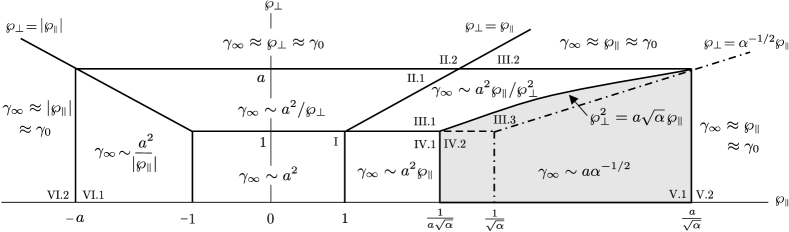
Regime	$w$ [Eq. (53)]	$\mathscr{P}_{y}$ [Eq. (55)]	$\Pi$ [Eq. (52)]	$\gamma_{\infty}$ [Eq. (49)]
I	$w\approx 1$	$\mathscr{P}_{y}\sim a$	$\Pi\approx 1$	$\gamma_{\infty}\sim a^{2}$
II.1	$w\approx\wp_{\perp}$	$\mathscr{P}_{y}\sim a$	$\Pi\approx\wp_{\perp}$	$\gamma_{\infty}\sim a^{2}/\wp_{\perp}$
II.2	$w\approx\wp_{\perp}$	$\mathscr{P}_{y}\approx\wp_{\perp}$	$\Pi\approx\wp_{\perp}$	$\gamma_{\infty}\approx\wp_{\perp}\approx\gamma_{0}$
III.1	$w\approx\wp_{\perp}^{2}/(2\wp_{{\scriptscriptstyle|{\kern-1.0pt}|}})$	$\mathscr{P}_{y}\sim a$	$\Pi\approx\wp_{\perp}^{2}/(2\wp_{{\scriptscriptstyle|{\kern-1.0pt}|}})$	$\gamma_{\infty}\sim a^{2}\wp_{{\scriptscriptstyle|{\kern-1.0pt}|}}/\wp_{\perp}^{2}$
III.2	$w\approx\wp_{\perp}^{2}/(2\wp_{{\scriptscriptstyle|{\kern-1.0pt}|}})$	$\mathscr{P}_{y}\approx\wp_{\perp}$	$\Pi\approx\wp_{\perp}^{2}/(2\wp_{{\scriptscriptstyle|{\kern-1.0pt}|}})$	$\gamma_{\infty}\approx\wp_{{\scriptscriptstyle|{\kern-1.0pt}|}}\approx\gamma_{0}$
III.3	$w\approx\wp_{\perp}^{2}/(2\wp_{{\scriptscriptstyle|{\kern-1.0pt}|}})$	$\mathscr{P}_{y}\sim a$	$\Pi\sim a\alpha^{1/2}$	$\gamma_{\infty}\sim a\alpha^{-1/2}$
IV.1	$w\approx 1/(2\wp_{{\scriptscriptstyle|{\kern-1.0pt}|}})$	$\mathscr{P}_{y}\sim a$	$\Pi\approx 1/(2\wp_{{\scriptscriptstyle|{\kern-1.0pt}|}})$	$\gamma_{\infty}\sim a^{2}\wp_{{\scriptscriptstyle|{\kern-1.0pt}|}}$
IV.2	$w\approx 1/(2\wp_{{\scriptscriptstyle|{\kern-1.0pt}|}})$	$\mathscr{P}_{y}\sim a$	$\Pi\approx 1/(2\wp_{{\scriptscriptstyle|{\kern-1.0pt}|}})$	$\gamma_{\infty}\sim a\alpha^{-1/2}$
V.1	$w\approx\alpha\wp_{{\scriptscriptstyle|{\kern-1.0pt}|}}/2$	$\mathscr{P}_{y}\sim a$	$\Pi\sim a\alpha^{1/2}$	$\gamma_{\infty}\sim a\alpha^{-1/2}$
V.2	$w\approx\alpha\wp_{{\scriptscriptstyle|{\kern-1.0pt}|}}/2$	$\mathscr{P}_{y}\sim\max\{\wp_{\perp},\,a\}$	$\Pi\approx\alpha\wp_{{\scriptscriptstyle|{\kern-1.0pt}|}}/2$	$\gamma_{\infty}\approx\wp_{{\scriptscriptstyle|{\kern-1.0pt}|}}\approx\gamma_{0}$
VI.1	$w\approx 2|\wp_{{\scriptscriptstyle|{\kern-1.0pt}|}}|$	$\mathscr{P}_{y}\sim a$	$\Pi\approx 2|\wp_{{\scriptscriptstyle|{\kern-1.0pt}|}}|$	$\gamma_{\infty}\sim a^{2}/|\wp_{{\scriptscriptstyle|{\kern-1.0pt}|}}|$
VI.2	$w\approx 2|\wp_{{\scriptscriptstyle|{\kern-1.0pt}|}}|$	$\mathscr{P}_{y}\sim\max\{\wp_{\perp},\,a\}$	$\Pi\approx 2|\wp_{{\scriptscriptstyle|{\kern-1.0pt}|}}|$	$\gamma_{\infty}\approx|\wp_{{\scriptscriptstyle|{\kern-1.0pt}|}}|\approx\gamma_{0}$

Figure 3: Regimes of ponderomotive acceleration for electrons born inside laser field with initial momentum ${\boldsymbol{\rm\wp}}$. The dashed and dot-dashed lines separate different domains corresponding to the same energy $\gamma_{\infty}$. The dot-dashed line is also a schematic of the curve (69), at which the particle velocity equals the pulse group velocity. Shaded is the “plateau” where the maximum energy $\gamma_{\infty}\sim a\alpha^{-1/2}$ is independent of ${\boldsymbol{\rm\wp}}$. The roman numbers are the same as for the corresponding domains in Fig. 2.

IV.3 Acceleration in vacuum

Suppose that an electron is produced at rest, e.g., due to ionization ref:hu02 ; ref:hu06 ; then, from Eq. (55),

$$\mathscr{P}_{\perp}=a_{0}\equiv a\cos\theta_{0}\sim a.$$ (57)

At $\alpha\ll 1$, the pulse travels much faster than the particle; hence the weak dispersion due to plasma is inessential in this case. Then Eq. (52) yields $\Pi\approx w=1$, so $\xi\sim a\sqrt{\alpha}\ll 1$ and $\Pi^{2}\gg\alpha(1+\mathscr{P}_{\perp}^{2})$, both because of Eq. (56). Therefore particle reflection from the pulse is impossible in this case (Sec. III.4), and Eq. (51) applies, yielding

$$\gamma_{\infty}=1+a_{0}^{2}/2,$$ (58)

in agreement with LABEL:my:gev and regime I in Fig. 3.

When a particle is born with positive $\wp_{{\scriptscriptstyle|{\kern-1.0pt}|}}\gg 1$, stronger acceleration is predicted from Eq. (51) due to reduced $\Pi$. Indeed, suppose a small pitch angle $\chi_{0}\approx\wp_{\perp}/\wp_{{\scriptscriptstyle|{\kern-1.0pt}|}}$ and, again, neglect the plasma dispersion ($\alpha\to 0$); then

$$w\approx\frac{1+\wp_{\perp}^{2}}{2\wp_{{\scriptscriptstyle|{\kern-1.0pt}|}}}\ll 1.$$ (59)

Similarly, Eq. (51) holds, so one gets

$$\gamma_{\infty}\approx\frac{\mathscr{P}_{y}^{2}\wp_{{\scriptscriptstyle|{\kern-1.0pt}|}}}{1+\wp_{\perp}^{2}}\sim\frac{a^{2}\wp_{{\scriptscriptstyle|{\kern-1.0pt}|}}}{1+\chi_{0}^{2}\wp^{2}_{{\scriptscriptstyle|{\kern-1.0pt}|}}},$$ (60)

covering regimes III.1 and IV.1 in Fig. 3. Hence only a small fraction of electrons is accelerated efficiently, particularly those with $\chi_{0}\lesssim\wp_{{\scriptscriptstyle|{\kern-1.0pt}|}}^{-1}\ll 1$. However, the maximum energy now scales as $\gamma_{\infty}\sim a^{2}\wp_{{\scriptscriptstyle|{\kern-1.0pt}|}}$, which is bigger than that flowing from Eq. (58) by the factor $\wp_{{\scriptscriptstyle|{\kern-1.0pt}|}}\gg 1$.

Specifically, the described effect is anticipated at large-angle electron-ion collisions in tenuous plasmas ref:balakin06 . Suppose a cold electron oscillating in a laser field with a quiver kinetic momentum $\bar{p}_{\sim}\sim a$ and zero average velocity. (For the general case, see Fig. 3 and Sec. V.) Suppose further that this particle collides with an ion such that the momentum vector instantaneously rotates toward the pulse propagation direction, i.e.,

$$\wp_{{\scriptscriptstyle|{\kern-1.0pt}|}}\approx\bar{p}_{\sim},\quad\wp_{\perp}\approx\bar{p}_{\sim}\chi_{0}.$$ (61)

Then the maximum $\gamma_{\infty}$ from Eq. (60) reads

$$\gamma_{\infty}\sim a^{3},$$ (62)

the result being called the $a^{3}$-effect ref:balakin06 , and the angular spread of the accelerated electrons is

$$\chi\approx\mathscr{P}_{\perp}/\gamma_{\infty}\sim a^{-2}\ll 1.$$ (63)

IV.4 Modification of the $\boldsymbol{a}^{\boldsymbol{3}}$-effect in plasma

Increasing the number of accelerated electrons requires higher plasma densities, and the $a^{3}$-effect is modified in this case because of the laser dispersion; hence the energy gain is calculated differently. Particularly, for electrons with the initial conditions (61), one has ${w\sim a^{-1}}$ [Eq. (59); regime IV] and ${q_{y}\sim 1}$; then Eq. (54) yields $\Pi^{2}\sim\max\{\alpha a^{2},\,a^{-2}\}$. At ${\sigma\equiv\alpha a_{\rm max}^{4}\ll 1}$ (regime IV.1), one obtains $\Pi\sim a^{-1}$, so the reflection condition is not met, and the plasma effect is negligible. Suppose now that $\sigma\gtrsim 1$ (regime IV.2). Then one gets

$$\Pi\sim a\sqrt{\alpha},$$ (64)

so it becomes possible to reflect electrons from the pulse, at least, for some $\theta_{0}$. (In vacuum, this effect is impossible because particles could not travel faster than light.) Hence the final energy is estimated from Eq. (50) as

$$\gamma_{\infty}\sim a\alpha^{-1/2},$$ (65)

and the angular spread of the accelerated electrons is

$$\chi\approx\mathscr{P}_{\perp}/\gamma_{\infty}\sim\sqrt{\alpha}\ll 1.$$ (66)

Now rewrite Eq. (65) as $\gamma_{\infty}\sim a^{3}\sigma^{-1/2}$. Then a uniform scaling is obtained, which covers both regimes IV.1 and IV.2, accounting for how the $a^{3}$-effect is modified with the plasma density:

$$\gamma_{\infty}\sim a^{3}\times\min\{1,\,\sigma^{-1/2}\}.$$ (67)

This agrees with the results of our numerical simulations. Specifically, at $\sigma\ll 1$ we observed the vacuum $a^{3}$-effect, and electron reflection from a pulse was seen at

$$\alpha a_{\rm max}^{4}\gtrsim 4.4.$$ (68)

Hence a sharp dependence of $\gamma_{\infty}$ on whether particles are reflected or not [albeit the scaling holds for reflected and transmitted electrons equaly, as predicted from Eqs. (49), (50)] and the abrupt elevation in Figs. 4, 5, both agreeing with Eqs. (65), (67).

Figure 4: The final energy $\gamma_{\infty}=p_{x}/mc$ of electrons accelerated by a plane laser pulse in tenuous plasma vs. the normalized vector potential envelope $a=e\mathcal{A}/mc^{2}$ at collision and cosine of the collision phase $\theta_{0}$; ${\alpha=10^{-3}}$, $a_{\rm max}=15$. The elevation corresponds to the electrons being snow-plowed.

Figure 5: Same as in Fig. 4 for $\theta_{0}=0$, with $a_{\rm max}=10$. (a) ${\alpha=10^{-4}}$: numerical (solid) and analytical, $\gamma_{\infty}=a^{3}$, corresponding to the $a^{3}$-effect (dashed); no particle reflection from the pulse. (b) ${\alpha=10^{-3}}$ (numerical); the elevation corresponds to the electrons being snow-plowed.

V Plateau regime

V.1 Maximum energy gain

Now consider a more realistic case when the electron is also preaccelerated by the pulse before the collision; hence we assume arbitrary initial conditions instead of Eq. (61). Similarly to Sec. IV.4, one can show that the acceleration is affected by plasma only in regimes III.3, IV.2, V.I, and V.2 (Fig. 3). Those adjoin the curve

$$\wp_{{\scriptscriptstyle|{\kern-1.0pt}|}}=\sqrt{\frac{1+\wp_{\perp}^{2}}{\alpha}},$$ (69)

which corresponds to the particle traveling at the pulse group velocity, with $\wp_{\perp}\ll\wp_{{\scriptscriptstyle|{\kern-1.0pt}|}}$ (dot-dashed in Fig. 3). Hence the respective interactions are classified as follows.

• In regimes III.3 and IV.2, a particle initially travels along $x$-axis slower than the pulse and is accelerated up to the energy (65).

• In regime V.I, a particle initially travels along $x$-axis faster than the pulse. However, it gains additional transverse momentum before it escapes from the field, resulting in the same energy gain (65).

• In regime V.2, a particle is fast enough to run ahead of the pulse such that the energy $\gamma$ is not affected ($\gamma_{\infty}\approx\gamma_{0}$), as opposed to vacuum where $\gamma_{\infty}\approx\gamma_{0}a^{2}$ would apply at arbitrarily large $\gamma_{0}$ (cf. IV.1).

• In all other regimes, the particle gains energy smaller than both $\gamma_{0}$ and that given by Eq. (65).

Thus for an electron born inside a laser field one has

$$\gamma_{\infty}\lesssim\max\{\gamma_{0},\,\Gamma\},$$ (70)

where $\Gamma\sim a\gamma_{g}$ is the energy of a particle comoving with the pulse, with the transverse momentum ${\bar{p}_{\perp}\sim a\gg 1}$ and the group velocity Lorentz factor ${\gamma_{g}=\alpha^{-1/2}}$.

Assuming $\gamma_{0}<\Gamma$, the maximum (over $\theta_{0}$) of the particle final energy is then attained in the “plateau” formed by the domains III.3, IV.2, V.I, where it is independent of the initial momentum ${\boldsymbol{\rm\wp}}$ and so is the angular spread of the accelerated electrons:

$$\gamma_{\infty}\sim a\gamma_{g},\quad\chi\sim\gamma_{g}^{-1}.$$ (71)

Below we assess the feasibility of the plateau regime and suggest an estimate for the energy of hot electrons which can be produced in conceivable experiments.

V.2 Required parameters

The one-dimensional (1D) model above neglects electron escape from the accelerating field in the transverse direction. This is a valid approximation if

$$\Delta\bar{\tau}\lesssim kL_{\perp}/\bar{p}_{\perp},$$ (72)

where $\Delta\bar{\tau}\sim\Delta\Psi/\dot{\Psi}$ is the normalized proper time of the interaction, and $\Delta\Psi\sim 1$ because the acceleration occurs on a single period (Sec. IV.2). In the plateau regime, Eq. (43) yields ${\dot{\Psi}\sim a\sqrt{\alpha}}$; thus Eq. (72) rewrites as

$$L_{\perp}/\lambda\gtrsim\big{(}2\pi\sqrt{\alpha}\,\big{)}^{-1},$$ (73)

where we took $\lambda$ for the laser wavelength, and ${\bar{p}_{\perp}\sim a}$. For narrower pulses, the energy gain would be somewhat lower than that predicted by Eq. (71), particularly for particles born at $\bar{A}\ll a_{\rm max}$, as also confirmed in our numerical simulations (Fig. 6). Nonetheless one can anticipate the 1D scaling to hold for feasibly focused ultraintense fields down to about $\alpha\sim 10^{-4}$. Hence the laser dispersion should affect the electron acceleration at plasma densities down to about $10^{17}\,\text{cm}^{-3}$.

Now let us estimate the influence of the previously neglected wake potential $\varphi$, which impedes the acceleration because the associated electrostatic force is directed oppositely to the ponderomotive force ref:du00 ; ref:esirkepov06 ; ref:shvets00 . The energy gain due to the electric field ${\boldsymbol{\rm E}}_{\varphi}=-\nabla\varphi$ is $\gamma_{\varphi}\sim eE_{\varphi}L/mc^{2}$, where $L\sim k^{-1}\Delta\bar{\tau}\gamma_{\infty}$ is the interaction length, or $kL\sim\gamma_{g}^{2}$. Assuming the wake spatial scale of about the plasma wavelength $\lambda_{p}=(k\sqrt{\alpha}\,)^{-1}$ and the density perturbation of the order of $n$, the Poisson’s equation gives $a_{\varphi}\equiv eE_{\varphi}/(mc\omega)\sim\sqrt{\alpha}$. Then $\gamma_{\varphi}\sim a_{\varphi}\,kL\sim\alpha^{-1/2}$, yielding $\gamma_{\varphi}/\gamma_{\infty}\sim a^{-1}\ll 1$, i.e., the wake is indeed negligible foot:intlength .

Hence Eq. (71) is a valid approximation for estimating the electron final energy. For example, at laser intensity $I\sim 10^{20}\,\text{W}/\text{cm}^{2}$ and wavelength $\lambda\sim 1\,\mu\text{m}$, corresponding to $a\approx[\lambda/(1\,\mu\text{m})][I/(1.37\times 10^{18}\,\text{W}/\text{cm}^{2})]^{1/2}\sim 10$, and $n\sim 10^{17}\,\text{cm}^{-3}$, corresponding to $\alpha\sim 10^{-4}$, Eqs. (71) predict $\gamma_{\infty}\sim 10^{3}$ and $\chi\sim 0.01$. Therefore hot electrons can be accelerated to energies of a fraction of GeV and will be scattered within a small angle of $0.6^{\circ}$.

Figure 6: Same as in Fig. 4 for $\theta_{0}=0$ and $a_{\rm max}=10$, but for a two-dimensional pulse $a=a_{\rm max}\exp(-x^{2}/L_{{\scriptscriptstyle|{\kern-1.0pt}|}}^{2}-y^{2}/L_{\perp}^{2})$ with $L_{{\scriptscriptstyle|{\kern-1.0pt}|}}=11\lambda$ and different $\ell\equiv L_{\perp}/\lambda$, where $\lambda=2\pi/k$.

VI Conclusions

In this paper, we derive the oscillation-center Hamiltonian for an electron injected with an arbitrary momentum in a linearly polarized laser pulse propagating in tenuous plasma, assuming that the pulse length $L_{{\scriptscriptstyle|{\kern-1.0pt}|}}$ is smaller than the plasma wavelength $\lambda_{p}$. We then use this formalism to describe the ponderomotive acceleration of hot electrons generated at collisions with ions under intense laser drive. Specifically, we identify multiple regimes of this acceleration and show that the laser dispersion affects the process at plasma densities down to $10^{17}\,\text{cm}^{-3}$. Assuming $a/\gamma_{g}\ll 1$ [Eq. (56)], which prevents net acceleration of the cold plasma, we also show that the normalized energy $\gamma$ of electrons accelerated from the initial energy $\gamma_{0}\lesssim\Gamma$ does not exceed $\Gamma\sim a\gamma_{g}$, where $a$ is the normalized laser field, and $\gamma_{g}$ is the group velocity Lorentz factor. Simultaneously, $\gamma\sim\Gamma$ is attained in a wide range of initial conditions, with the angular spread of the accelerated electrons ${\chi\sim\gamma_{g}^{-1}}$. Hence the distribution of hot electrons produced at large-angle collisions with ions at $L_{{\scriptscriptstyle|{\kern-1.0pt}|}}\ll\lambda_{p}$ and $a/\gamma_{g}\ll 1$ will have a cutoff at $\gamma\sim a\gamma_{g}$. This refines the result from LABEL:ref:balakin06, showing how even weak laser dispersion can affect the acceleration gain. However, further experiments are yet needed to validate the updated scaling, because no relevant data has been reported for the regime considered here.

VII Acknowledgments

This work was supported by the Russian Foundation for Basic Research through Grant No. 08-02-01209-a and the NNSA under the SSAA Program through DOE Research Grant No. DE-FG52-04NA00139.

Appendix A Energy gain in vacuum

In the case of vacuum, a simplified solution is possible as follows. Perform a canonical transformation foot:intact

$$(\bar{x},\rho;\,\bar{t},-\gamma)\to(\theta,\rho^{\prime};\,\eta,-w)$$ (74)

using a generating function

$$\digamma=(\bar{x}-\bar{t})\rho^{\prime}-\bar{t}{\kern 0.7pt}w.$$ (75)

Then

$$\theta=\bar{x}-\bar{t},\quad\rho^{\prime}=\rho,\quad\eta=\bar{t},\quad w=\gamma-\rho,$$ (76)

and the transformed extended Hamiltonian is given by

$$h^{\prime}=1-w^{2}-2w\rho^{\prime}+\mathscr{P}_{z}^{2}+\big{\{}\mathscr{P}_{y}-a(\epsilon\theta)\,\cos\theta\big{\}}^{2}\equiv 0.$$

Then $w$ is conserved, yielding an explicit solution for $\rho$:

$$\rho=\frac{1}{2w}\Big{[}1-w^{2}+\mathscr{P}_{z}^{2}+\big{\{}\mathscr{P}_{y}-a(\epsilon\theta)\,\cos\theta\big{\}}^{2}\Big{]}.$$ (77)

Hence the particle energy $\gamma=\rho+w$ is obtained, and outside the field one has [cf. Eq. (51)]

$$\gamma_{\infty}=\frac{1+w^{2}+\mathscr{P}_{\perp}^{2}}{2w}.$$ (78)

References

- (1) G. A. Mourou, T. Tajima, and S. V. Bulanov, Rev. Mod. Phys. 78, 309 (2006).
- (2) S. P. D. Mangles, B. R. Walton, M. Tzoufras, Z. Najmudin, R. J. Clarke, A. E. Dangor, R. G. Evans, S. Fritzler, A. Gopal, C. Hernandez-Gomez, W. B. Mori, W. Rozmus, M. Tatarakis, A. G. R. Thomas, F. S. Tsung, M. S. Wei, and K. Krushelnick, Phys. Rev. Lett. 94, 245001 (2005).
- (3) S.-Y. Chen, M. Krishnan, A. Maksimchuk, R. Wagner, and D. Umstadter, Phys. Plasmas 6, 4739 (1999).
- (4) A. A. Balakin and G. M. Fraiman, Zh. Eksp. Teor. Fiz. 130, 426 (2006) [JETP 103, 370 (2006)].
- (5) M. Eloy, A. Guerreiro, J. T. Mendonça, and R. Bingham, J. Plasma Phys. 73, 635 (2006).
- (6) J. T. Mendonça, L. O. Silva, and R. Bingham, J. Plasma Phys. 73, 627 (2007).
- (7) J. T. Mendonça, Plasma Phys. Control. Fusion 51, 024007 (2009).
- (8) C. J. McKinstrie and E. A. Startsev, Phys. Rev. E 54, R1070 (1996).
- (9) C. J. McKinstrie and E. A. Startsev, Phys. Rev. E 56, 2130 (1997).
- (10) C. Du and Z. Xu, Phys. Plasmas 7, 1582 (2000).
- (11) E. A. Startsev and C. J. McKinstrie, Phys. Plasmas 10, 2552 (2003).
- (12) N. S. Ginzburg and M. D. Tokman, Fiz. Plazmy 8, 884 (1982) [Sov. J. Plasma Phys. 8, 501 (1982)].
- (13) N. S. Ginzburg and M. D. Tokman, Zh. Tech. Fiz. 57, 409 (1987) [Sov. Phys. Tech. Phys. 32, 249 (1987)].
- (14) J. M. Rax, Phys. Fluids B 4, 3962 (1992).
- (15) M. D. Tokman, Fiz. Plazmy 25, 160 (1999) [Plasma Phys. Rep. 25, 140 (1999)].
- (16) L. D. Landau and E. M. Lifshitz, The classical theory of fields (Pergamon Press, New York, 1971).
- (17) I. Y. Dodin and N. J. Fisch, Phys. Plasmas 13, 103104 (2006).
- (18) C. D. Decker and W. B. Mori, Phys. Rev. E 51, 1364 (1995).
- (19) P. Sprangle, E. Esarey, and A. Ting, Phys. Rev. Lett. 64, 2011 (1990).
- (20) The numerical simulations reported in LABEL:ref:startsev03 confirm that the linear plasma model is reasonably accurate for calculating the electron ponderomotive acceleration by a laser pulse with and .
- (21) The dispersion (7) due to plasma [book:jackson , Sec. 7.9] can also be attributed to a waveguide structure [book:jackson , Sec. 8.3].
- (22) The transverse variables remain intact, so the corresponding terms in the generating functions are omitted.
- (23) V. I. Arnold, V. V. Kozlov, and A. I. Neishtadt, Dynamical Systems III (Springer-Verlag, New York, 1988).
- (24) R. L. Dewar, Phys. Fluids 16, 1102 (1973).
- (25) S. Johnston, A. N. Kaufman, and G. L. Johnston, J. Plasma Phys. 20, 365 (1978).
- (26) S. Johnston and A. N. Kaufman, J. Plasma Phys. 22, 105 (1979).
- (27) I. Y. Dodin and N. J. Fisch, Phys. Rev. E 77, 036402 (2008).
- (28) I. Y. Dodin and N. J. Fisch, arXiv:0811.2010 (2008).
- (29) A. V. Gaponov and M. A. Miller, Zh. Eksp. Teor. Fiz. 34, 242 (1958) [Sov. Phys. JETP 7, 168 (1958)].
- (30) H. Motz and C. J. H. Watson, Adv. Electron. 23, 153 (1967).
- (31) J. R. Cary and A. N. Kaufman, Phys. Rev. Lett. 39, 402 (1977).
- (32) T. W. B. Kibble, Phys. Rev. 150, 1060 (1966).
- (33) D. Bauer, P. Mulser, and W. H. Steeb, Phys. Rev. Lett. 75, 4622 (1995).
- (34) A. Bourdier and S. Gond, Phys. Rev. E 63, 036609 (2001).
- (35) B. Quesnel and P. Mora, Phys. Rev. E 58, 3719 (1998).
- (36) I. Y. Dodin, N. J. Fisch, and G. M. Fraiman, Pis’ma Zh. Eksp. Teor. Fiz. 78, 238 (2003) [JETP Lett. 78, 202 (2003)].
- (37) J. M. Rax and N. J. Fisch, Phys. Rev. Lett. 69, 772 (1992).
- (38) Eq. (40) is not accurate enough to predict the actual reflection point at (except at ); e.g., Fig. 1 shows no common solution for Eq. (40) and Eq. (44) at . On the other hand, at , the latter equations yield , which agrees with the results of our single-particle simulations.
- (39) I. Y. Dodin and N. J. Fisch, Phys. Rev. E 68, 056402 (2003).
- (40) S. X. Hu and A. F. Starace, Phys. Rev. Lett. 88, 245003 (2002).
- (41) S. X. Hu and Anthony F. Starace, Phys. Rev. E 73, 066502 (2006).
- (42) T. Esirkepov, S. V. Bulanov, M. Yamagiwa, and T. Tajima, Phys. Rev. Lett. 96, 014803 (2006).
- (43) G. Shvets, N. J. Fisch, and A. Pukhov, IEEE Trans. Plasma Sci. 28, 1185 (2000).
- (44) For interaction on the whole pulse length (), one can similarly obtain . Thus, for ultrashort intense pulses, is, again, negligible.
- (45) J. D. Jackson, Classical electrodynamics (Wiley, New York, 1975).