A perturbative nonequilibrium renormalization group method for dissipative quantum mechanics

Abstract

We study a generic problem of dissipative quantum mechanics, a small local quantum system with discrete states coupled in an arbitrary way (i.e. not necessarily linear) to several infinitely large particle or heat reservoirs. For both bosonic or fermionic reservoirs we develop a quantum field-theoretical diagrammatic formulation in Liouville space by expanding systematically in the reservoir-system coupling and integrating out the reservoir degrees of freedom. As a result we obtain a kinetic equation for the reduced density matrix of the quantum system. Based on this formalism, we present a formally exact perturbative renormalization group (RG) method from which the kernel of this kinetic equation can be calculated. It is demonstrated how the nonequilibrium stationary state (induced by several reservoirs kept at different chemical potentials or temperatures), arbitrary observables such as the transport current, and the time evolution into the stationary state can be calculated. Most importantly, we show how RG equations for the relaxation and dephasing rates can be derived and how they cut off generically the RG flow of the vertices. The method is based on a previously derived real-time RG technique hs_koenig_PRL00 ; keil_hs_PRB01 ; hs_lecture_notes_00 ; korb_reininghaus_hs_koenig_PRB07 but formulated here in Laplace space and generalized to arbitrary reservoir-system couplings. Furthermore, for fermionic reservoirs with flat density of states, we make use of a recently introduced cutoff scheme on the imaginary frequency axis jakobs_meden_hs_PRL07 which has several technical advantages. Besides the formal set-up of the RG equations for generic problems of dissipative quantum mechanics, we demonstrate the method by applying it to the nonequilibrium isotropic Kondo model. We present a systematic way to solve the RG equations analytically in the weak-coupling limit and provide an outlook of the applicability to the strong-coupling case.

1 Introduction

General remarks. Dissipative quantum mechanics is a fundamental field in theoretical physics combining the concepts of quantum mechanics and nonequilibrium statistical mechanics diss_QM . The aim is to develop a microscopic description of how a small quantum-mechanical system in contact with large reservoirs (see Fig.1 for a sketch of the system) evolves into a stationary state and what this stationary state looks like. In equilibrium statistical mechanics for large quantum systems in contact with a single reservoir, the strength and nature of the system-reservoir interaction is not important, since it is a surface effect and negligible compared to the bulk of the quantum system. Therefore, in this case, depending on which conserved quantities are exchanged, the stationary state is always a canonical or grandcanonical ensemble. For quantum systems in contact with several reservoirs which are kept at different temperatures or chemical potentials (inhomogeneous boundary conditions), the stationary state is a nonequilibrium state and possibly current-carrying. However, if the quantum system is large, again only the interactions in the bulk are important which can be treated perturbatively via standard quantum Boltzmann equations QBE . After a short crossover time local equilibrium establishes and the further time evolution can be described by hydrodynamic equations Hydro . These standard tools of nonequilibrium statistical mechanics break down for small quantum systems for several reasons.

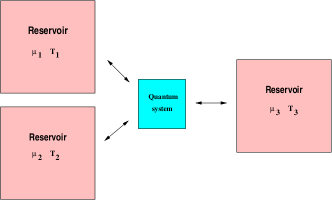
Figure 1: A small quantum system coupled to several infinitely large reservoirs via energy and/or particle exchange. The reservoirs are characterized by temperatures $T_{i}$ and chemical potentials $\mu_{i}$.

First the system-reservoir coupling is no longer a negligible surface effect but can change the states on the system considerably via quantum fluctuations. Even for weak coupling renormalization of the coupling parameters and the level positions of the quantum system can occur at low temperatures. Strinkingly new effects can occur for strong coupling such as a localization transition in the spin-boson model diss_QM or resonant transmission for a local spin coupled via exchange to reservoir spins (the so-called Kondo effect) kondo_exp ; kondo_theo . Secondly, it becomes energetically difficult to put several electrons on the quantum system due to the large capacitive interaction $E_{C}\sim e^{2}/L$ ($L$ being the length of the quantum system), the so-called charging energy. Typical experimental values for semiconductor quantum dots, metallic islands or carbon nanotubes are $E_{C}\sim 1-10\mbox{K}$ and much larger than typical temperatures $T\sim 10-100\mbox{mK}$ (for single molecules coupled to leads the charging energy can be even larger reaching typical atomic values). A simple perturbative expansion in the interaction is no longer possible and usual quantum Boltzmann equations can not be used. Furthermore, for low-dimensional systems, the Coulomb interaction can lead to completely new physical phenomena such as Luttinger liquid behaviour in 1-dimensional quantum wires Luttinger . Concepts like local equilibrium are not applicable. Phase coherence is maintained over the whole system size and the quantum system acts like a scattering region for electrons entering and leaving the system rather than a region where particles can relax, dephase and equilibrate.

For these reasons, new theoretical tools have been developed to understand relaxation, dephasing, and nonequilibrium quantum transport through small quantum systems coupled to external reservoirs. For noninteracting systems, the standard tool is the Landauer-Büttiker formalism landauer_buettiker where the particle current is expressed by the scattering matrix together with the occupation of the scattering waves determined by the chemical potentials of the reservoirs. In this case, it is possible to consider arbitrary coupling between reservoirs and quantum system and the coherent properties of the quantum system are fully taken into account. For interacting systems (or systems with spin degrees of freedom), the situation is much more complicated and no unique analytical or numerical formalism is available which can cover all regimes of interest. Numerical methods for nonequilibrium are currently been developed, such as time-dependent density matrix renormalization group (TD-DMRG) TD-DMRG , time-dependent numerical renormalization group TD-NRG , numerical renormalization group at finite bias voltage using scattering waves nonequilibrium-NRG , quantum Monte Carlo with complex chemical potentials QMC , and iterative path-integral approaches thorwart_egger . Exact solutions using scattering Bethe-ansatz are available for the resonant level model bethe . Concerning analytical methods two perturbative approaches are commonly used, depending on whether one expands in the interaction parameter inside the quantum system or in the reservoir-system coupling. Expanding in the interaction has the advantage that the unperturbed part of the Hamiltonian is quadratic in the field operators and standard Keldysh-Green’s function techniques can be applied caroli ; jauho . Furthermore, rather large quantum systems can be treated since the effort scales with the number of single-particle levels rather than with the number of many-particle states. However, this method has its limitations since for typical quantum dots the Coulomb interaction is the largest energy scale of the problem. In contrast, expanding in the reservoir-system coupling has the advantage that arbitrary interaction strength on the quantum sytem can be treated. Furthermore, the reservoir-system coupling is often tunable in experiments and in most cases the lowest energy scale. Therefore it seems reasonable to expand around the point where reservoirs and quantum system are decoupled. In this case the unperturbed part of the Hamiltonian contains the full interacting quantum system and standard Green’s function techniques can not be applied (a generic problem for all strongly correlated systems). One way out of this problem is the use of slave particle techniques where the interacting system is expressed in a quadratic form using creation and annihilation operators of many-particle states slave_particles_general ; barnes . Standard Keldysh-Green’s function methods can then be used by expanding in the reservoir-system coupling slave_particles_wingreen . However, technical complications arise due to an additional constraint for the slave particle number and, most importantly, diagrammatic approximations are often doubtful due to the unphysical nature of the slave particles. So even the noninteracting case is quite nontrivial barnes and vertex corrections are essential to obtain the relaxation and dephasing rates for the physical particles paaske_rosch_kroha_woelfle_PRB04 . In contrast, the most standard method of dissipative quantum mechanics is to integrate out only the noninteracting reservoirs and describe the dynamics of the reduced density matrix of the quantum system via a kinetic equation. This can be achieved by projection operator techniques in Liouville space zwanzig or via path-integral methods diss_QM ; grifoni . Most recently, a quantum field-theoretical version of this strategy has been developed in Refs. hs_schoen_PRB94 ; koenig_hs_schoen_EPL95 ; koenig_schmid_hs_schoen_PRB96 , see Ref. hs_habil for a review. The advantage is that Wick’s theorem is used to integrate out the reservoirs and an exact diagrammatic representation of the kernel determining the kinetic equation is obtained. This allows for a direct calculation of this kernel in terms of irreducible diagrams whereas with projection operator techniques the calculation is complicated by cancellations of reducible expressions. Furthermore, the usage of representations similiar to Feynman diagrams simplifies the implementation of renormalization group ideas.

RG for the Kondo model. The analytical methods expanding either in the interaction or the reservoir-system coupling can of course be used to calculate all physical quantities of interest in perturbation theory. In this way many time-dependent and nonequilibrium phenomena have been described in various fields, such as spin boson models, quantum optics, mesoscopic systems, quantum information theory, etc. However, perturbation theory is often plagued by various diverging terms in higher orders if some low energy scale like temperature, voltage, magnetic field, etc. becomes too small. In this limit perturbation theory becomes ill-defined and the natural question arises whether renormalization group methods can be generalized to the nonequilibrium situation to resum the original perturbation theory in an appropriate way so that it becomes well-defined again. To be specific let us introduce a simple but nontrivial example, the nonequilibrium Kondo model. This model is currently one of the basic unsolved problems of nonequilibrium condensed matter physics and serves as an important benchmark model for theoreticians to test the applicability of their nonequilibrium techniques. The model consists of the most simplest fermionic quantum system one can imagine, namely a spin-${1\over 2}$ system, which interacts with two fermionic reservoirs (being kept at temperature $T$ and two different chemical potentials $\mu_{L}$ and $\mu_{R}$) via exchange processes, see Fig.2.

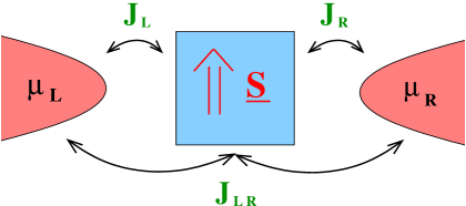
Figure 2: A spin-${1\over 2}$ quantum system coupled via exchange to two reservoirs. $J_{L}=J_{LL}$ and $J_{R}=J_{RR}$ involve exchange between the spins of the left/right reservoir with the local spin, and $J_{LR}=J_{RL}$ transfers a particle from one reservoir to the other during the exchange process.

The Hamiltonian for the reservoir-system coupling reads

$$V\,=\,{1\over 2}\sum_{\alpha\alpha^{\prime}=L,R}\,\,\,\sum_{\sigma\sigma^{\prime}=\uparrow,\downarrow}\,\,\sum_{kk^{\prime}}\,J_{\alpha\alpha^{\prime}}\,\underline{S}\cdot\underline{\sigma}_{\sigma\sigma^{\prime}}\,\,a^{\dagger}_{\alpha\sigma k}a_{\alpha^{\prime}\sigma^{\prime}k^{\prime}}\quad.$$ (1)

Here, $\underline{S}$ denotes the spin operator of the quantum system, $\underline{\sigma}$ are the Pauli matrices, and $a,a^{\dagger}$ are the fermionic annihilation and creation operators for the particles in the reservoirs characterized by reservoir index $\alpha=L,R$, spin $\sigma=\uparrow,\downarrow$ and state index $k$. The exchange couplings are denoted by $J_{\alpha\alpha^{\prime}}$. For a symmetric system, there are only two different exchange couplings

$$J_{d}=J_{LL}=J_{RR}\quad,\quad J_{nd}=J_{LR}=J_{RL}\quad.$$ (2)

The diagonal exchange coupling $J_{d}$ characterizes spin exchange which involves only the spin of one reservoir, whereas the nondiagonal coupling $J_{nd}$ describes a process where one particle is transferred between the reservoirs (see e.g. Ref. korb_reininghaus_hs_koenig_PRB07 for a derivation of this form of the interaction via a standard Schrieffer-Wolff transformation from a conventional tunneling Hamiltonian). The latter process leads to a particle current at finite bias. For simplicity we consider only the isotropic case without magnetic field. The reservoirs are characterized by a noninteracting Hamiltonian

$$H_{res}\,=\,\sum_{\alpha=L,R}\,\,H_{\alpha}\,=\,\sum_{\alpha=L,R}\,\,\epsilon_{\alpha\sigma k}\,\,a^{\dagger}_{\alpha\sigma k}a_{\alpha\sigma k}\quad,$$ (3)

and the statistics is given by an equilibrium grandcanonical distribution

$$\rho_{res}\,=\,\prod_{\alpha=L,R}\,\,\rho_{\alpha}\quad,\quad\rho_{\alpha}\,=\,{1\over Z_{\alpha}}\,e^{-{1\over T_{\alpha}}(H_{\alpha}-\mu_{\alpha}N_{\alpha})}\quad,$$ (4)

where $T_{L}=T_{R}=T$ denotes the temperature and $\mu_{L}=-\mu_{R}=V/2$ the chemical potentials of the reservoirs ($V$ is the bias voltage and we use units $e=\hbar=1$).

Even in equilibrium $V=0$ the Kondo model is a highly nontrivial model and numerous many-body techniques have been used to study its properties, see e.g. hewson for a review. We summarize here shortly its basic properties and consider the simplest case $J=J_{d}=J_{nd}$. Higher-order perturbation theory in $J$ for transition rates (or the linear conductance) leads generically to logarithmic divergencies $\sim(J\,\mbox{ln}(D/\Lambda_{c}))^{n}$, where $D$ denotes the bandwidth of the reservoirs and $\Lambda_{c}\sim T$ is the low-energy scale. For the linear conductance, the logarithmic terms start in $O(J^{3})$

$$G\,=\,G_{0}\,{3\pi^{2}\over 4}\,J^{2}\,(1+4J\,\mbox{ln}(D/\Lambda_{c}))\quad,$$ (5)

with $G_{0}=2e^{2}/h$. To resum the most divergent terms in each order of perturbation theory (the so-called leading-order analysis), poor man scaling methods have been developed poor_man_scaling where the high energy scales of the reservoirs are successively integrated out. If $\Lambda$ denotes the effective bandwidth of the reservoirs (with initial value $D$), an infinitesimal reduction $\Lambda\rightarrow\Lambda-d\Lambda$ is compensated by a renormalization of the exchange coupling $J$ while keeping the scattering t-matrix invariant (in leading order). As a result one finds the so-called poor man scaling equation (valid for $J\ll 1$)

$${dJ\over d\Lambda}\,=\,-{2J^{2}\over\Lambda}\quad,$$ (6)

with the solution

$$J(\Lambda)\,=\,{1\over 2\,\mbox{ln}(\Lambda/T_{K})}\quad,\quad T_{K}\,=\,\Lambda\,e^{-{1\over 2J}}\quad,$$ (7)

where $T_{K}$ denotes the Kondo temperature which is an invariant of the RG equation (6). In the antiferromagnetic case $J>0$, the effective coupling diverges at $\Lambda=T_{K}$ indicating a complete screening of the local spin by the reservoir spins. This leads to a spin-singlet ground state and it can be shown that the remaining potential scattering terms lead to unitary conductance (Kondo effect). The Kondo effect has been measured for semiconductor quantum dots, carbon nanotubes, and molecules kondo_exp (for theoretical works see Refs. kondo_theo ; slave_particles_wingreen ; koenig_schmid_hs_schoen_PRB96 or Ref. glazman_pustilnik_05 for a review). This is the so-called strong-coupling regime where the perturbative RG equation (6) is no longer valid. However, the poor man scaling equation has to be cut off by the low-energy scale $\Lambda_{c}\sim T$ and the strong coupling regime can not be reached for $\Lambda_{c}\gg T_{K}$. The weak coupling regime is defined by $J_{c}=J(\Lambda_{c})\ll 1$, where perturbation theory has to be carried out in the renormalized coupling $J_{c}$ with an effective bandwidth given by $\Lambda_{c}$. Replacing $J\rightarrow J_{c}$ and $D\rightarrow\Lambda_{c}$ in (5), one obtains

$$G\,=\,G_{0}\,{3\pi^{2}\over 4}\,J_{c}^{2}\,=\,G_{0}\,{3\pi^{2}\over 16}\,{1\over\mbox{ln}^{2}(T/T_{K})}\quad.$$ (8)

Since $J_{c}$ is logarithmically increased compared to the bare coupling $J_{0}=J(D)$, the onset of the Kondo effect is indicated by a logarithmic enhancement of the conductance as function of temperature. Note that simple perturbation theory in the original coupling $J_{0}$ can already break down in this regime since the two conditions

$$J_{0}\,\mbox{ln}(D/\Lambda_{c})\,=\,{1\over 2}-J_{0}\,\mbox{ln}(\Lambda_{c}/T_{K})\,\sim\,O(1)\quad\mbox{and}\quad J_{c}\,=\,{1\over 2\mbox{ln}(\Lambda_{c}/T_{K})}\,\ll\,1$$ (9)

can easily be fulfilled, provided that $1\ll\mbox{ln}(\Lambda_{c}/T_{K})\ll 1/J_{0}$ (although the typical experimental situation is rarely strictly in this regime, it provides a well-defined regime where perturbative renormalization group methods can be tested).

In nonequilibrium $V\neq 0$ and $V>T$, the situation is not so clear. The standard poor man scaling procedure suggests that the low-energy scale $\Lambda_{c}$ is given by the maximum of $T$ and $V$, i.e. the voltage serves as a cutoff parameter in the same way as temperature. Alternatively it was conjectured in Ref. coleman that $J_{d}$ is cut off by $T$ (since it involves only the spins of one reservoir) and $J_{nd}$ is cut off by $\mbox{max}\{T,V\}$, opening up the possibility of a strong-coupling fixed point for $V\gg T_{K}\gg T$. Finally, in Refs. kaminski_etal ; rosch_kroha_woelfle_PRL01 it was proposed that also spin relaxation and dephasing rates can cut off the RG flow. For the isotropic Kondo model in the absence of a magnetic field the relaxation and dephasing rates are the same and are given by the Korringa rate

$$\Gamma\,=\,\pi\,J^{2}\,\mbox{max}\{T,V\}\quad.$$ (10)

This has the consequence that $\Gamma\gg T_{K}$ if $V\gg T_{K}$ (note that $T_{K}$ is exponentially small for $J\ll 1$ whereas $\Gamma$ scales quadratic with $J$) and a strong-coupling fixed point can not be reached for $V\gg T_{K}\gg T$. In this paper we will provide a microscopic nonequilibrium RG approach clarifying all these issues. Indeed, it turns out that the Korringa rate cuts off the RG flow of $J_{d}$ and $J_{nd}$. Roughly the poor man scaling equation (6) has to be replaced by the RG equations (see Eqs. (579) and (580) of Sec. 5.3)

$${dJ_{d}\over d\Lambda} = -\theta_{T}\,\left({J_{d}^{2}\over\Lambda+\Gamma}+J_{nd}^{2}\,\,\mbox{Re}{1\over\Lambda+\Gamma+iV}\right)\quad,$$ (11)

$${dJ_{nd}\over d\Lambda} = -\theta_{T}\,J_{d}J_{nd}\,\,\mbox{Re}\left\{{1\over\Lambda+\Gamma}+{1\over\Lambda+\Gamma+iV}\right\}\quad,$$ (12)

with $\theta_{T}=\theta(\Lambda-T)$, where we have omitted additional frequency dependencies of the vertices (see Sec. 5.3 for more details where also the RG equation for $\Gamma$ is shown). As one can see, temperature and Korringa rate cut off all terms on the r.h.s of the RG equation whereas the voltage is only present in certain terms. This shows that nonequilibrium induces new features into the RG equations. Neither $J_{d}$ nor $J_{nd}$ are completely cut off by the voltage and from these RG equations alone there is no justification to cut off the RG flow by the voltage if $V>T$. Instead, the RG flow should be cut off by $\Gamma$ leading to additional $J_{c}^{2}\,\mbox{ln}(J_{c})$ contributions for the exchange couplings. However, as will be discussed in detail in Sec. 5.3, there is an additional RG equation for the current rate which is cut off by the voltage and not by $\Gamma$. As a consequence the cutoff parameter which enters into the conductance is indeed the voltage and we obtain precisely the result (8) with temperature replaced by bias voltage. However, it is important to recognize that the fact that $\Gamma$ does not enter the final result for the conductance does not mean that it can be neglected. For $T=0$ and $V\gg T_{K}$, the RG equations (11) and (12) would diverge for $\Lambda\rightarrow 0$ if the cutoff parameter $\Gamma$ were not present, leading also to a divergence of the conductance since the RG equation for the current rate is cut off smoothly by the voltage, see Sec. 5.3. Therefore, it is an important issue for nonequilibrium RG methods to incorporate the physics of relaxation and dephasing rates into the RG equations.

The situation becomes even more interesting if an additional energy scale $\Delta$ is present, such as magnetic field, external driving frequency, level spacing, charge excitation energy etc. In this case, it turns out that additional logarithmic terms can occur which are generically of the form $\mbox{ln}(D/|n{V\over 2}-\Delta|)$ with $n$ being an integer number, see Sec. 4.3 and Refs. reininghaus_hs_preprint ; oppen_1 . At $V=2\Delta/n$ these logarithmic terms diverge corresponding to certain resonance positions. Relaxation and dephasing rates will also cut off these divergencies. Thus, their effect is two-fold: relaxation and dephasing rates cut off the RG flow for the vertices and also the RG flow for all physical observables, such as the current rate, susceptibilities, occupation probabilities, etc. Furthermore, an interesting question is what happens in the strong-coupling regime, where the RG flow of the relaxation and dephasing rates is cut off by themselves. It is expected that they saturate to the Kondo temperature and prevent the RG flow from diverging. This issue is discussed in Sec. 5.3.

RG methods. Motivated by these considerations and due to the progress in experimental techniques to study quantum transport through small nanodevices, there is an increased interest in the development of renormalization group methods for nonequilibrium systems (which are either driven out of equilibrium with an external bias or are prepared in an out of equilibrium initial state). The first proposal for a nonequilibrium RG technique, commonly called real-time RG (RTRG), was provided in Ref. hs_koenig_PRL00 for problems of dissipative quantum mechanics, see Ref. hs_lecture_notes_00 for a tutorial introduction. The method is perturbative in the reservoir-system coupling and is based on the diagrammatic kinetic equation approach reviewed in Ref. hs_habil . Instead of the bandwidth, the relative time of the reservoir Green’s function was used as a cutoff parameter and the kernel of the kinetic equation was kept invariant during the RG flow by setting up a formally exact hierarchy of RG equations. The method has been applied to charge fluctuations in the single electron box koenig_hs_PRL98 , transport through metallic quantum dots pohjola_koenig_hs_schoen_PRB99 ; hs_koenig_kuczera_schoen_JLTP00 , charge fluctuations in semiconductor quantum dots hs_koenig_PRL00 ; boese_hofstetter_hs_PRB01 , the polaron problem keil_hs_PRB00 , the influence of acoustic phonons on transport through coupled quantum dots keil_hs_PRB02 , and to the dynamics of the spin boson problem keil_hs_PRB01 . Within all these applications, a linear coupling between the quantum system and the particle or heat reservoir was considered. In this case, it was sufficient to use the RG method with a cutoff defined in time space. For models like the nonequilbrium Kondo model, where spin fluctuations are important, a quadratic coupling involving one creation and one annihilation operator of the reservoirs occurs, see (1). To treat this case in a convenient way, a version of the RTRG method with a cutoff defined in real frequency space has been developed recently korb_reininghaus_hs_koenig_PRB07 . An essential ingredient of these techniques is the generation of non-Hamiltonian dynamics during the RG flow in terms of an effective Liouville operator of the quantum system with nonzero imaginary parts of its eigenvalues representing the relaxation and dephasing rates. This effective Liouville operator appears also in the RG equations of the vertices cutting them off at these energy scales. However, a problem of this approach is the fact that a certain time-ordering procedure has to be defined for the renormalized vertices which leads to the generation of terms which are not present in the original perturbation theory and have to be corrected by counter terms in higher orders. This leads to the problem that the cutoff of the RG flow by relaxation and dephasing rates can only be seen in leading order and a proof that this effect happens in all orders is not possible (leaving the question open whether a strong-coupling fixed point is in principle possible). In addition, it is not unambigiously clear what the precise scale of the rates cutting off the RG flow is. Finally, concerning the numerical stability for solving the RG equations, it turns out that cutoff functions which are defined in real time or real frequency space are not the best choice. In this paper, we will show how these problems can be circumvented by some new technical tricks which have been used recently in Ref. reininghaus_hs_preprint to calculate analytically the nonlinear conductance, the magnetic susceptibility, the spin relaxation and dephasing rates, and the renormalized g-factor up to 2-loop order for the nonequilibrium anisotropic Kondo model at finite magnetic field in the weak-coupling regime. The first technical step is to show that the RG approach can be set up purely in frequency space korb_private_communication using the diagrammatic rules of Ref. hs_habil . As a consequence the occurence of correction terms can be avoided and the rates determining the cutoff of the RG flow obtain the right scale. Secondly, it turns out that it is important to integrate out the symmetric part of the Fermi or Bose distribution function of the reservoirs before starting the RG flow. With this choice it is possible to show generically for all models of dissipative quantum mechanics that relaxation and dephasing rates cut off the RG flow in all orders of perturbation theory and within all truncation schemes of the RG equations. Another technical advantage is that the dependence on the Keldysh indices can be avoided, minimizing the effort to solve the RG equations. Finally, it is more convenient to define a cutoff not in real but in imaginary frequency space by introducing the cutoff into the Matsubara poles of the reservoir distribution function. This idea was first proposed in Ref. jakobs_meden_hs_PRL07 in the context of nonequilibrium functional renormalization group within the Keldysh formalism. This choice improves the numerical stability considerably. Furthermore, for fermionic reservoirs with a flat density of states, it is possible to reformulate the RG equations in pure Matsubara space (all integrals over the real frequencies can be performed analytically) with the difference to equilibrium that a whole set of Matsubara axis occurs shifted by multiples of the chemical potentials of the reservoirs and by the real part of the Laplace variable determining the time evolution of the system. With this technique it is possible to provide a generic procedure how to solve the RG equations analytically in a well-controlled way in the weak-coupling regime, see Ref. reininghaus_hs_preprint . Whether it is also applicable to the strong-coupling regime is an open question discussed in Sec. 5.3 for the special case of the nonequilibrium isotropic Kondo model. For later reference, we will call this version of nonequilibrium RG real-time RG in frequency space (RTRG-FS).

Especially for the Kondo model, the development of nonequilibrium RG has been pioneered in Refs. rosch_kroha_woelfle_PRL01 ; rosch_paaske_kroha_woelfle_PRL03 (for perturbation theory see Refs. paaske_rosch_woelfle_PRB04 ; paaske_rosch_kroha_woelfle_PRB04 ; a poor man scaling approach is described in Ref. glazman_pustilnik_05 ). In these works the slave particle approach was used in connection with Keldysh formalism and quantum Boltzmann equations. A real-frequency cutoff was used and the RG was formulated purely on one part of the Keldysh-contour disregarding diagrams connecting the upper with the lower branch. This procedure turns out to be sufficient for the Kondo model to calculate logarithmic terms in leading order but the cutoff by relaxation and dephasing rates can not be obtained in this way. In these works it was investigated for the first time how the voltage and the magnetic field cuts off the RG flow and how the frequency dependence of the vertices influences various logarithmic contributions $\sim\mbox{ln}({\mbox{max}(V,h)\over|V-h|})$ or $\sim\mbox{ln}({V\over h})$ for the susceptibility and the nonlinear conductance.

An alternative approach to RTRG-FS for combining relaxation and dephasing rates microscopically with nonequilibrium RG was proposed in Ref. kehrein_PRL05 using flow-equation methods flow_eq . Specifically for the isotropic Kondo model without magnetic field it was shown that the cutoff of the RG flow by the decay rate $\Gamma$ occurs due to a competition of 1-loop and 2-loop terms on the r.h.s. of the RG equation for the vertex. This is a completely different picture compared to RTRG-FS, where the cutoff parameter $\Gamma$ occurs already in the 1-loop terms as an additional term in the denominator of the resolvents, see the RG-equations (11) and (12). Thus, RTRG-FS is closer to conventional poor man scaling equations and the physics of relaxation and dephasing rates occurs naturally as a resummation of a geometric series similiar to self-energy insertions in Green’s function techniques. Nevertheless, the flow equation method is well-definied and controlled, and represents a technical alternative to RTRG-FS.

Nonequilibrium RG methods which expand perturbatively in the Coulomb interaction of the quantum system have also been developed recently jakobs_meden_hs_PRL07 ; gezzi_pruschke_meden_PRB07 ; jakobs_diplom ; jakobs_pletyukhov_hs_preprint . In these works, the Keldysh formalism has been combined with functional RG techniques known from quantum field theory wetterich ; salmhofer . It turns out that a real-frequency cutoff is not useful since it violates causality and leads to various numerical instabilites jakobs_diplom ; gezzi_pruschke_meden_PRB07 . For fermionic models in 1d a more useful cutoff scheme on the imaginary frequency axis has been proposed jakobs_meden_hs_PRL07 , which is also very useful for RTRG-FS (see the discussion above). An interesting result was obtained that Luttinger liquid exponents can depend on the nonequilibrium distribution function of the quantum system jakobs_meden_hs_PRL07 . For zero-dimensional systems (quantum dots) with a single spin-degenerate level coupled by tunneling to two reservoirs (the so-called single-impurity Anderson model), the situation is more complicated because there is no controlled truncation scheme for a perturbative RG in the Coulomb interaction $U$, especially in the interesting regime where the Coulomb interaction becomes larger than the energy scale $\Gamma$ of the reservoir-system coupling. Furthermore, the Green’s function in the absence of the Coulomb interaction has a pole in the complex plane with imaginary part $\Gamma$ (corresponding to energy broadening of the dot level due to coupling to the reservoirs). This pole is close to the real-axis compared to the cutoff-parameter of the RG flow. As a consequence the cutoff procedure defined on the Matsubara axis is not sufficient for this problem and $\Gamma$ itself was proposed as the flowing cutoff parameter jakobs_pletyukhov_hs_preprint . With this choice it is possible to study the nonequilibrium Anderson impurity-model up to values of $U\sim 2-4\Gamma$ even in the Kondo regime $T,V\ll T_{K}$ jakobs_pletyukhov_hs_preprint (the truncation scheme in this work neglects the 3-particle vertex but takes the important parts of the frequency-dependence of the 2-particle vertex into account). For $U\gg\Gamma$ charge fluctuations are suppressed and the model is equivalent to the Kondo model with $J\sim\Gamma/U$. However, it is not yet possible to approach the limit $J\ll 1$, where the Kondo temperature shows the typical exponential behaviour. It remains an interesting and open question whether this approach can be improved and a full solution of the nonequilibrium Anderson-impurity model including the nonequilibrium Kondo model can be obtained.

Finally, we mention that in this introduction we have only summarized the nonequilibrium RG approaches relevant for problems of dissipative quantum mechanics. There is also a rapidly increasing interest in the development of nonequilibrium RG methods for bulk quantum systems motivated by the interesting possibilities to measure the time evolution of strongly correlated quantum systems in cold atom gases. For completeness we mention some of the most interesting recent developments, e.g. the study of quantum phase transitions in nonequilibrium millis ; berges , the far-from-equilibrium quantum field dynamics of ultracold atom systems gasenzer_pawlowski , and the time-evolution of fermionic system after initial interaction quenches moeckel_kehrein_PRL08 .

Outline. The present paper concentrates on the scheme of RTRG-FS which is especially useful for a generic study of problems in dissipative quantum mechanics, where the expansion parameter is the reservoir-system coupling. We will describe the formal technique for a generic model but will always accompany the formalism by an illustration for fermionic models where charge, spin or orbital fluctuations dominate. Especially we will apply the formalism in all details to the nonequilibrium isotropic Kondo model. The paper is written for students with some basic knowledge of many-body theory. Besides second quantization and Wick’s theorem nothing special is required. The paper is organized as follows. In Sec. 2 we will introduce the generic model and some specific examples. In Sec. 3 we present a nonequilibrium quantum field-theoretical diagrammatic description in Liouville space by introducing creation and annihilation superoperators acting in Liouville space (i.e. with an additional Keldysh-index). This is especially useful for obtaining compact diagrammatic rules. Based on this diagrammatic expansion we present a derivation of a formally exact kinetic equation for the reduced density matrix of the quantum system and provide the rules to calculate observables. In Sec. 4 we develop the nonequilibrium RG approach. We discuss the general idea of invariance, various ways to define the cutoff function, and set up simple rules to obtain the RG equations in arbitrary order in the coupling. We discuss their general properties and prove the central theorem that the RG flow is always cut off by relaxation and dephasing rates. For fermionic models with spin or orbital fluctuations, following Ref. reininghaus_hs_preprint , we will describe the generic scheme how to solve the RG equations analytically in the weak-coupling regime. Finally, in Sec. 5 we apply the technique to the nonequilibrium isotropic Kondo model, show the results of Ref. reininghaus_hs_preprint in 1-loop order, and present preliminary results for the strong-coupling case. We close with a summary and an outlook in Sec. 6.

2 The model

2.1 Generic case

Generically any Hamiltonian of a problem in dissipative quantum mechanics can be decomposed into a part for the reservoirs, the local quantum system, and the coupling between reservoirs and quantum system

$$H\,=\,H_{res}\,+\,H_{S}\,+\,V\,=\,H_{0}\,+\,V\quad.$$ (13)

The unperturbed part is denoted by

$$H_{0}\,=\,H_{res}\,+\,H_{S}\quad.$$ (14)

For the local quantum system $H_{S}$ we make no assumption and represent it via its eigenstates $|s\rangle$ and eigenenergies $E_{s}$

$$H_{S}\,=\,\sum_{s}\,E_{s}\,|s\rangle\langle s|\quad.$$ (15)

In practice the eigenstates $|s\rangle$ can easily be found for a quantum system with a low number of single particle states including arbitrary interactions. In reality each quantum system has an infinite number of states. However, if the system is very small (as we assume) the single particle level spacing is very large and high-lying states can be neglected (for sufficiently small temperature and bias voltage). Therefore, it is often sufficient to take only a few single-particle levels into account and $H_{S}$ can be easily diagonalized. Since we want to include the possibility that particles can be exchanged between reservoirs and quantum system, the states have to be classified according to their particle number. We denote by $N_{s}$ the particle number for state $|s\rangle$. We include both possibilities that the particles can be bosons or fermions. E.g. bosonic particles can be realized in cold atom gases whereas fermionic particles (electrons) occur typically in nanoelectronic systems.

The reservoirs are assumed to be noninteracting and infinitely large with a continuum density of states. Therefore, we use a continuum notation for the creation and annihilation operators of the particles in the reservoirs and the reservoir Hamiltonian reads in second quantization

$$H_{res}\,=\,\sum_{\alpha}H_{\alpha}\,=\,\sum_{\nu\equiv\alpha\sigma\dots}\int d\omega\,(\omega+\mu_{\alpha})\,a^{\dagger}_{\nu}(\omega)a_{\nu}(\omega)\quad,$$ (16)

with the continuum commutation relations for the field operators

$$[a_{\nu}(\omega),a^{\dagger}_{\nu^{\prime}}(\omega^{\prime})]_{\mp}\,=\,\delta_{\nu\nu^{\prime}}\delta(\omega-\omega^{\prime})\quad,$$ (17)

where the upper (lower) sign correponds to bosons (fermions) and $[A,B]_{\mp}=AB\mp BA$ is the (anti-)commutator. $\nu$ is a discrete index which labels all remaining quantum numbers of the reservoir particles

$$\nu\,=\,\alpha\sigma\dots\quad,$$ (18)

where, by convention, $\alpha$ is the index numerating the reservoirs (e.g. $\alpha=L,R\equiv\pm$ for two reservoirs) and $\sigma$ is the spin index (e.g. $\sigma=\uparrow,\downarrow\equiv\pm$ for a spin-${1\over 2}$ system). Further possibilities are orbital indices (if orbital symmetries are present), channel indices (for transverse modes), etc. The chemical potential of reservoir $\alpha$ is denoted by $\mu_{\alpha}$, and $\omega$ is the energy of the reservoir state measured relative to $\mu_{\alpha}$ (for phonon or photon baths, the chemical potential is absent). The reservoirs are assumed to be described by a grandcanonical distribution function

$$\rho_{res}\,=\,\prod_{\alpha}\,\rho_{\alpha}\quad,\quad\rho_{\alpha}\,=\,{1\over Z_{\alpha}}\,e^{-{1\over T_{\alpha}}(H_{\alpha}-\mu_{\alpha}N_{\alpha})}\quad,$$ (19)

where $T_{\alpha}$ is the temperature of reservoir $\alpha$.

We note that the crossover from a discrete to a continuum notation for the reservoir field operators can be formally achieved by the definition

$$a_{\nu}(\omega)\,=\,{1\over\sqrt{\rho_{\nu}(\omega)}}\sum_{k}\,\delta(\omega-\epsilon_{\nu k}+\mu_{\alpha})\,a_{\nu k}\quad,$$ (20)

where $k$ is a discrete index labelling the states of the reservoirs, $\epsilon_{\nu k}$ is their corresponding energy, and $\rho_{\nu}(\omega)$ is the density of states in reservoir $\alpha$ (which can depend on energy and possibly (for ferromagnetic leads) on the spin index). It is easy to show that with this definition the reservoir Hamiltonian (16) in the continuum form is equivalent to the discrete version

$$H_{res}\,=\,\sum_{\nu k}\,\epsilon_{\nu k}\,a_{\nu k}^{\dagger}a_{\nu k}\quad.$$ (21)

Thereby, we have assumed that the relation between $k$ and $\epsilon_{\nu k}$ is unique, otherwise different branches of the dispersion relation have to be distinguished and labelled by additional indices.

For later convenience we introduce the following more compact notation for the various indices characterizing the reservoir field operators

$$1\,\equiv\,\eta\nu\omega\quad,\quad a_{1}\,\equiv\,a_{\eta\nu}(\omega)\,=\,\left\{\begin{array}[]{cl}a_{\nu}^{\dagger}(\omega)&\mbox{for }\eta=+\\ a_{\nu}(\omega)&\mbox{for }\eta=-\end{array}\right.\,\quad.$$ (22)

Here, $\eta=\pm$ indicates either a creation or annihilation operator. If no ambiguities occur we use $1\equiv\eta\nu\omega$ and $1^{\prime}\equiv\eta^{\prime}\nu^{\prime}\omega^{\prime}$, whereas for several indices we take $1\equiv\eta_{1}\nu_{1}\omega_{1}$, $2\equiv\eta_{2}\nu_{2}\omega_{2}$, etc. Furthermore we define by

$$\bar{1}\equiv-\eta,\nu\omega\quad,\quad a_{\bar{1}}\,=\,(a_{1})^{\dagger}\quad,$$ (23)

the index corresponding to the hermitian conjugate. With these notations the commutation relation (17) can be written in the compact form

$$[a_{1},a_{1^{\prime}}]_{\mp}\,=\,\delta_{1\bar{1}^{\prime}}\quad,$$ (24)

where $\delta_{11^{\prime}}$ stands for

$$\delta_{11^{\prime}}\,\equiv\,\delta_{\eta\eta^{\prime}}\delta_{\nu\nu^{\prime}}\delta(\omega-\omega^{\prime})\quad.$$ (25)

In all expressions we sum (integrate) implicitly over the indices, i.e. we sum over the discrete part $\eta$ and $\nu$, and integrate over the continuum variable $\omega$. The reservoir Hamiltonian can be written in the compact form

$$H_{res}\,=\,(\omega+\mu_{\alpha})\,\delta_{1\bar{1}^{\prime}}\,\delta_{\eta+}\,a_{1}a_{1^{\prime}}\quad,$$ (26)

and the reservoir correlation function (also called reservoir contraction) reads

$${a_{1}\,a_{1^{\prime}}\begin{picture}(-20.0,11.0)\put(-22.0,8.0){\line(0,1){3.0}} \put(-22.0,11.0){\line(1,0){12.0}} \put(-10.0,8.0){\line(0,1){3.0}} \end{picture}\begin{picture}(20.0,11.0)\end{picture}}\,\equiv\,\langle a_{1}a_{1^{\prime}}\rangle_{\rho_{res}}\,=\,\delta_{1\bar{1}^{\prime}}\,f^{\eta}_{\alpha}(\omega)\,=\,\delta_{1\bar{1}^{\prime}}\,\left\{\begin{array}[]{cl}\eta\\ 1\end{array}\right\}\,f_{\alpha}(\eta\omega)\quad,$$ (27)

where $f_{\alpha}^{+}(\omega)\equiv f_{\alpha}(\omega)$, $f_{\alpha}^{-}(\omega)\equiv 1\pm f_{\alpha}(\omega)$, and

$$f_{\alpha}(\omega)\,=\,{1\over e^{\omega/T_{\alpha}}\mp 1}\,=\,\mp\,f_{\alpha}^{-}(-\omega)$$ (28)

is the Bose (Fermi) function corresponding to temperature $T_{\alpha}$ (note that the chemical potential $\mu_{\alpha}$ does not occur in this formula because $\omega$ measures the energy relative to $\mu_{\alpha}$). The upper (lower) case in (27) refers to bosons (fermions), a convention which we will use throughout this paper.

For the coupling between reservoirs and quantum system we take the generic form

$$V\,=\,{1\over n!}\,\,g_{12\dots n}:a_{1}\,a_{2}\,\dots\,a_{n}:\quad,$$ (29)

where $g_{12\dots n}$ is an arbitrary operator acting on the quantum system, and we sum implicitly over $n=1,2,\dots$ and all variables $\eta_{i},\nu_{i},\omega_{i}$, $i=1,2,\dots,n$, which are contained in the formal notation $i\equiv\eta_{i},\nu_{i},\omega_{i}$. We note that we explicitly exclude the case $n=0$ because this corresponds to an operator of the local quantum system which can be incorporated in $H_{S}$. The symbol $:\dots:$ denotes normal-ordering of the reservoir field operators with respect to the reservoir correlation function, i.e. in any Wick-decomposition of an average over a sequence of reservoir field operators with respect to $\rho_{res}$, no contraction is allowed which connects field operators occuring in the same normal-ordered block. As a consequence the average over a normal-ordered block is defined as zero $\langle:a_{1}a_{2}\dots a_{n}:\rangle_{\rho_{res}}=0$. The field operators within the normal-ordering can be arranged in an arbitrary order (up to a sign for fermions). The prefactor ${1\over n!}$ accounts for all permutations of reservoir field operators which do not change the value of the diagrams in perturbation theory (see later) since the coupling vertex can always be chosen such that it is (anti)symmetric under exchange of two indices

$$g_{1\dots i\dots j\dots n}\,=\,\pm\,g_{1\dots j\dots i\dots n}\quad.$$ (30)

For simplicity, we assume here that either fermionic or bosonic field operators occur for the reservoirs. If both are present (e.g. for combinations of electronic particle reservoirs and phonon heat baths), one simply writes the coupling as a sum of several terms, each one being of the form (29). In principle also mixed couplings can be treated containing fermionic and bosonic field operators in the same term but we will not consider this case here because it just complicates the notation (in this case there is a factor ${1\over n_{B}!\,n_{F}!}$ in front of Eq. (29), where $n_{B}$ ($n_{F}$) is the number of bosonic (fermionic) field operators).

The form (29) of the coupling includes all cases of charge, spin, and energy transfer between reservoirs and quantum system and, for $n>1$, also includes nonlinear coupling. The coupling vertex $g_{12\dots n}$ describes the change of the state of the quantum system and is an operator. We have included the possibility that it depends in an arbitrary way on the frequencies of the reservoir field operators. Although such a general form (especially for $n>2$) is hardly necessary for realistic models, this general form with all possible values for $n$ has to be considered since the RG procedure described in Sec. 4 will generate an effective coupling which includes all these terms.

The total operator $V$ is of bosonic nature since the parity of fermion number must be conserved. However, for fermions and $n$ odd, $g_{12\dots n}$ in (29) is of fermionic nature and the sequence of $g_{12\dots n}$ and $:a_{1}a_{2}\dots a_{n}:$ is important (the coupling $V$ in the form (29) is even not hermitian in this case). To be precise, in the general case $V$ should be written as

$$V\,=\,{1\over n!}\,\left\{\begin{array}[]{cl}1\\ \eta_{1}\dots\eta_{n}\end{array}\right\}\,:a_{n}a_{n-1}\dots a_{1}:\,\,g_{12\dots n}\quad.$$ (31)

With this choice it can easily be shown that $V$ is hermitian, provided the coupling vertex fulfils the condition

$$(g_{12\dots n})^{\dagger}\,=\,g_{\bar{n}\dots\bar{1}}\quad.$$ (32)

Furthermore, it is shown in Appendix A that the form (31) is only important for fixing the value of the coupling vertex $g_{1\dots n}$ for a concrete model. After having defined $g_{1\dots n}$ in this way, one can proceed with the much simpler form (29) and disregard all sign factors emerging from interchanging fermionic dot and reservoir operators. The reason is that by calculating the reduced density matrix of the quantum system or averages of observables, only expressions have to be evaluated where an average over the reservoir distribution $\rho_{res}$ is taken, for details see Appendix A. Thus, in the following we work with the simpler form (29) and commute dot and reservoir operators. This simplifies the problem of sign factors considerably.

Finally, we mention that it is sometimes more convenient to include the density of states of the reservoirs into the reservoir contraction (27). In this case we use the definition

$$b_{1}\,=\,\sqrt{\rho_{\nu}(\omega)}\,\,a_{1}\,\quad$$ (33)

for the reservoir field operator and obtain for the contraction

$${b_{1}\,b_{1^{\prime}}\begin{picture}(-20.0,11.0)\put(-20.0,9.0){\line(0,1){3.0}} \put(-20.0,12.0){\line(1,0){10.0}} \put(-10.0,9.0){\line(0,1){3.0}} \end{picture}\begin{picture}(20.0,11.0)\end{picture}}\,\equiv\,\langle b_{1}b_{1^{\prime}}\rangle_{\rho_{res}}\,=\,\delta_{1\bar{1}^{\prime}}\,\rho_{\nu}(\omega)\,f^{\eta}_{\alpha}(\omega)\quad.$$ (34)

Correspondingly, the coupling $V$ is written in the form

$$V\,=\,{1\over n!}\,\,g_{12\dots n}:b_{1}\,b_{2}\,\dots\,b_{n}:\quad,$$ (35)

where dot and reservoir operators commute, and

$$V\,=\,{1\over n!}\,\left\{\begin{array}[]{cl}1\\ \eta_{1}\dots\eta_{n}\end{array}\right\}\,:b_{n}b_{n-1}\dots b_{1}:\,\,g_{12\dots n}$$ (36)

for the determination of $g_{12\dots n}$.

2.2 Specific examples

Here, we present some specific and experimentally relevant examples for charge, spin, orbital, or energy fluctuations induced by the coupling between reservoirs and quantum system.

Charge fluctuations. Electronic quantum transport through nanodevices or quantum dots is characterized by charge fluctuations and is conveniently described by a tunneling Hamiltonian, i.e. the coupling is of the form

$$V\,=\,\sum_{\alpha\sigma}\sum_{k}\sum_{l}\,t^{\alpha\sigma}_{kl}\,a^{\dagger}_{\alpha\sigma k}\,c_{\sigma l}\,+\,(h.c.)\quad.$$ (37)

Here, $\alpha$ and $\sigma$ are the reservoir and spin indices, respectively, and $l$ is an index for an arbitrary single-particle state basis of the quantum system. $t^{\alpha\sigma}_{kl}$ are the tunneling matrix elements and $c_{\sigma l}$ annihilates a particle on the quantum system in state $l$ with spin $\sigma$. In the continuum notation and with $\nu\equiv\alpha\sigma$, we obtain

$$V\,=\,\sum_{\eta\nu}\int d\omega\,\eta\,a_{\eta\nu}(\omega)\,g_{\eta\nu}(\omega)\,\equiv\,\eta_{1}\,a_{1}\,g_{1}\quad,$$ (38)

with $a_{\eta\nu}(\omega)$ defined by (22) and (20), and the coupling vertex is given by

$$g_{\eta\nu}(\omega)\,=\,\sqrt{\rho_{\nu}(\omega)}\left\{\begin{array}[]{cl}\sum_{l}\,t^{\nu}_{l}(\omega)\,c_{\sigma l}&\mbox{for }\eta=+\\ \sum_{l}\,t^{\nu}_{l}(\omega)^{*}\,c^{\dagger}_{\sigma l}&\mbox{for }\eta=-\end{array}\right.\quad,$$ (39)

where $t^{\nu}_{l}(\omega)\equiv t^{\nu}_{kl}$ with $\omega=\epsilon_{\nu k}-\mu_{\alpha}$.

To obtain dimensionless coupling vertices, one can define for each $\nu$ and $\omega$ some reference tunneling matrix element $t^{\nu}(\omega)\equiv t^{\nu}_{k}$ (independent of the state index $l$ of the quantum system), with a corresponding level broadening parameter $\Gamma_{\nu}(\omega)$ defined by

$$\Gamma_{\nu}(\omega)\,=\,2\pi\,\rho_{\nu}(\omega)|t^{\nu}(\omega)|^{2}\,=\,2\pi\,\sum_{k}\,|t^{\nu}_{k}|^{2}\,\delta(\omega-\epsilon_{\nu k}+\mu_{\alpha})\quad.$$ (40)

With this reference energy, we define the dimensionless reservoir field operators

$$b_{\eta\nu}(\omega)\,=\,\sqrt{\Gamma_{\nu}(\omega)/(2\pi)}\,a_{\eta\nu}(\omega)\,=\,\left\{\begin{array}[]{cl}\sum_{k}\,|t^{\nu}_{k}|\,\delta(\omega-\epsilon_{\nu k}+\mu_{\alpha})\,a^{\dagger}_{\nu k}&\mbox{for }\eta=+\\ \sum_{k}\,|t^{\nu}_{k}|\,\delta(\omega-\epsilon_{\nu k}+\mu_{\alpha})\,a_{\nu k}&\mbox{for }\eta=-\end{array}\right.\quad,$$ (41)

and the corresponding dimensionless coupling vertex

$$g_{\eta\nu}(\omega)\,=\,\left\{\begin{array}[]{cl}\sum_{l}\,t^{\nu}_{l}(\omega)/|t^{\nu}(\omega)|\,c_{\sigma l}&\mbox{for }\eta=+\\ \sum_{l}\,t^{\nu}_{l}(\omega)^{*}/|t^{\nu}(\omega)|\,c^{\dagger}_{\sigma l}&\mbox{for }\eta=-\end{array}\right.\quad,$$ (42)

such that we obtain again the form (38) with $a\rightarrow b$. The reservoir contraction with respect to the $b$-operators reads

$${b_{1}\,b_{1^{\prime}}\begin{picture}(-20.0,11.0)\put(-20.0,9.0){\line(0,1){3.0}} \put(-20.0,12.0){\line(1,0){10.0}} \put(-10.0,9.0){\line(0,1){3.0}} \end{picture}\begin{picture}(20.0,11.0)\end{picture}}\,\equiv\,\langle b_{1}b_{1^{\prime}}\rangle_{\rho_{res}}\,=\,\delta_{1\bar{1}^{\prime}}\,{1\over 2\pi}\Gamma_{\nu}(\omega)\,f^{\eta}_{\alpha}(\omega)\quad.$$ (43)

Spin and orbital fluctuations. If the charging energy of a quantum dot is very large (compared to temperature and bias voltage), the gate voltage determining the position of the charge excitation energies of the quantum dot relative to the electrochemical potentials of the reservoirs can be adjusted such that charge fluctuations are suppressed. In this case, spin and orbital fluctuations dominate transport. The elementary processes are given by an electron tunneling on (off) the quantum system, occupying a virtual intermediate state, and in a second step tunneling off (on) the quantum system. As shown in detail in Ref. korb_reininghaus_hs_koenig_PRB07 , the virtual intermediate state (which has a very high energy due to the large charging energy) can be integrated out via a standard Schrieffer-Wolff transformation on a Hamiltonian level, and the result is a coupling of the form

$$V\,=\,{1\over 2}\,g_{11^{\prime}}\,:a_{1}a_{1^{\prime}}:\quad.$$ (44)

In most cases (except for systems with negative charging energies oppen_2 ), one creation and annihilation operator is present, i.e. $\eta=-\eta^{\prime}$ (note that the forms (29) and (31) are equivalent in this case).

Whereas (44) describes a generic model for spin and/or orbital fluctuations on a quantum dot, a special case is the Kondo model (1) discussed in the introduction. In this case, only fluctuations of a spin-${1\over 2}$ of the quantum system are considered and, comparing (44) with (1), we obtain for the dimensionless coupling vertex in the continuum form

$$g_{11^{\prime}}\,=\,{1\over 2}\,\left\{\begin{array}[]{cl}J_{\alpha\alpha^{\prime}}\,\underline{S}\cdot\underline{\sigma}_{\sigma\sigma^{\prime}}&\mbox{for }\eta=-\eta^{\prime}=+\\ -J_{\alpha^{\prime}\alpha}\,\underline{S}\cdot\underline{\sigma}_{\sigma^{\prime}\sigma}&\mbox{for }\eta=-\eta^{\prime}=-\end{array}\right.\quad,$$ (45)

such that the antisymmetry and hermiticity conditions

$$g_{11^{\prime}}\,=\,-g_{1^{\prime}1}\quad,\quad g_{11^{\prime}}^{\dagger}\,=\,g_{\bar{1}^{\prime}1}$$ (46)

are fulfilled, compare (30) and (32).

Since, due to the Schrieffer-Wolff transformation, high-lying charge excitations have already been integrated out in the model (44), one has to consider the reservoirs with a finite bandwidth $D$ (of the order of the charging energy). Thus, all frequencies $\omega$ have to be smaller than $D$, which can be achieved by various cutoff functions. In this paper, we will use a Lorentzian cutoff defined by the function

$$\rho(\omega)\,=\,{D^{2}\over\omega^{2}+D^{2}}\,=\,{D\over 2i}({1\over\omega-iD}-{1\over\omega+iD})\quad.$$ (47)

Most elegantly, we introduce this function by a modification of the reservoir contraction (27)

$${a_{1}\,a_{1^{\prime}}\begin{picture}(-20.0,11.0)\put(-22.0,8.0){\line(0,1){3.0}} \put(-22.0,11.0){\line(1,0){12.0}} \put(-10.0,8.0){\line(0,1){3.0}} \end{picture}\begin{picture}(20.0,11.0)\end{picture}}\,\rightarrow\,\delta_{1\bar{1}^{\prime}}\,\rho(\omega)\,f^{\eta}_{\alpha}(\omega)$$ (48)

Although this is not done here by a formal redefinition of the field operators, the effect of this modification of the reservoir correlation function is that all frequencies are suppressed if they lie above the band cutoff $D$. This will become clear within the diagrammatic expansion described in Sec. 3, where the reservoir degrees of freedom are integrated out.

Energy fluctuations. Within the traditional field of dissipative quantum mechanics, a heat bath or energy-exchange with the environment is considered, mostly within the so-called spin-boson model defined by the Hamiltonian

$$H_{res} = \sum_{q}\,\omega_{q}\,a^{\dagger}_{q}a_{q}\quad,$$ (49)

$$H_{S} = -{\Delta\over 2}\sigma_{x}\,+\,{\epsilon\over 2}\sigma_{z}\quad,$$ (50)

$$V = {1\over 2}\sigma_{z}\,\sum_{q}\,\gamma_{q}\,(a^{\dagger}_{q}+a_{q})\quad.$$ (51)

Here, the quantum system consists of a two-level system with tunneling coupling $\Delta$ between the two levels and bias $\epsilon$ determining the detuning. The bath consists of a set of harmonic oscillators (phonons) with bosonic creation and annihilation operators $a^{\dagger}_{q},a_{q}$. The phonon energy is $\omega_{q}>0$ and the bath couples linearly (via the spatial coordinate $\sim a^{\dagger}_{q}+a_{q}$) to the two-level system. The coupling parameters $\gamma_{q}$ and the density of states of the phonon modes are conventionally parametrized by the spectral function

$$J(\omega)\,=\,\pi\,\sum_{q}\,\gamma_{q}^{2}\,\delta(\omega-\omega_{q})\,=\,2\pi\,\alpha\,\omega^{n+1}\,e^{-\omega/D}\quad.$$ (52)

$n=0$ describes the important ohmic case, whereas $n>0$ and $n<0$ are called the super-ohmic and sub-ohmic case. $D$ is the bandwidth of the bath, and $\alpha$ describes the coupling parameter (which is dimensionless for the ohmic case).

For our continuum notation, we define in analogy to (41) the dimensionless bosonic field operators

$$b_{\eta}(\omega)\,=\,\left\{\begin{array}[]{cl}\sum_{q}\,g_{q}\,\delta(\omega-\omega_{q})\,a^{\dagger}_{q}&\mbox{for }\eta=+\\ \sum_{q}\,g_{q}\,\delta(\omega-\omega_{q})\,a_{q}&\mbox{for }\eta=-\end{array}\right.\quad,$$ (53)

and obtain with the dimensionless coupling vertex

$$g_{\pm}\,=\,{\sigma_{z}\over 2}$$ (54)

the form

$$V\,=\,g_{1}\,b_{1}$$ (55)

for the coupling, and

$${b_{1}\,b_{1^{\prime}}\begin{picture}(-20.0,11.0)\put(-20.0,9.0){\line(0,1){3.0}} \put(-20.0,12.0){\line(1,0){10.0}} \put(-10.0,9.0){\line(0,1){3.0}} \end{picture}\begin{picture}(20.0,11.0)\end{picture}}\,=\,\delta_{1\bar{1}^{\prime}}\,{1\over\pi}J(\omega)\,f^{\eta}(\omega)\quad$$ (56)

for the bath contraction, where $f^{+}(\omega)=f(\omega)$, $f^{-}(\omega)=1+f(\omega)$ and $f(\omega)=1/(e^{\beta\omega}-1)$ is the Bose function. Note that only positive frequencies $\omega$ are allowed since the phonon energies are positive.

Formally, one can rewrite the expressions such that both positive and negative frequencies are allowed by using the definiton

$$d_{\eta}(\omega)\,=\,\left\{\begin{array}[]{cl}b_{\eta}(\omega)&\mbox{for }\omega>0\\ b_{-\eta}(-\omega)&\mbox{for }\omega<0\end{array}\right.\quad.$$ (57)

Since $d_{\eta}(\omega)=d_{-\eta}(-\omega)$, we get

$$\sum_{\eta}\,\int_{0}^{\infty}d\omega\,b_{\eta}(\omega)\,=\,\sum_{\eta}\,\int_{0}^{\infty}d\omega\,d_{\eta}(\omega)\,=\,{1\over 2}\,\sum_{\eta}\,\int_{-\infty}^{\infty}d\omega\,d_{\eta}(\omega)\quad,$$ (58)

and $V$ can be written as (note that $g_{1}$ does not depend on $\eta$)

$$V\,=\,\bar{g}_{1}\,d_{1}\quad,\quad\bar{g}_{1}\,=\,{\sigma^{z}\over 4}\quad.$$ (59)

Using $f^{-}(\omega)=1+f(\omega)=-f(-\omega)$, we get for the contraction in the new representation

$${d_{1}\,d_{1^{\prime}}\begin{picture}(-20.0,11.0)\put(-20.0,9.0){\line(0,1){3.0}} \put(-20.0,12.0){\line(1,0){10.0}} \put(-10.0,9.0){\line(0,1){3.0}} \end{picture}\begin{picture}(20.0,11.0)\end{picture}}\,=\,\delta_{11^{\prime}}\,{1\over\pi}\,\mbox{sign}(\omega)\,J(|\omega|)\,f^{\eta}(\omega)\quad,$$ (60)

where all frequencies are allowed now.

3 Quantum field theory in Liouville space

In this section we will develop a quantum field-theoretical diagrammatic expansion in Liouville space. Conventional quantum field theory in nonequilibrium is based on the Keldysh-formalism, where all field operators are integrated out via Wick’s theorem or via Gaussian integrals within path integral formalism. This is not possible here because the unperturbed part of the Hamiltonian, consisting of the reservoirs $H_{res}$ and the quantum system $H_{S}$, contains arbitrary interaction terms in $H_{S}$. Therefore, this part is not quadratic and Wick’s theorem does not apply. For this reason, only the degrees of freedom of the reservoirs can be integrated out. However, the coupling vertex $g_{1\dots n}$ remains an operator and the dynamics between the vertices is described by $H_{S}$. Therefore, a diagrammatic representation is obtained where the vertices are operators and one has to keep track of their time-ordering on the Keldysh-contour. In contrast to previous versions of this procedure hs_lecture_notes_00 , we introduce here a slightly different way of integrating out the reservoirs. Instead of expanding the time evolution on the Keldysh contour and applying Wick’s theorem for the reservoir field operators, we will introduce quantum field superoperators acting in Liouville space for the reservoirs. This has the advantage that the two branches of the Keldysh contour can be taken together from the very beginning in a compact way. Subsequently, we will apply Wick’s theorem for the quantum field superoperators. This procedure combines in an efficient way the advantages of Liouville superoperators (the traditional formalism of dissipative quantum mechanics) and quantum field theory on the Keldysh contour (the common way to treat nonequilibrium systems). The traditional way of deriving kinetic equations by using projection operators in Liouville space zwanzig is a very formal procedure and much less useful. Although one obtains a very compact and analytic notation for the kernel of the kinetic equation without any need of a diagrammatic representation, the reservoirs are not integrated out and everything is hidden in formal projectors which finally have to be evaluated by decomposing all expressions into many artificial reducible terms where numerous cancellations occur. Integrating out the reservoirs from the very beginning has the advantage that the kernel can be defined via irreducible diagrams only and the calculations simplify considerably. Furthermore, it is shown in Sec. 4 that a systematic renormalization group method generates an additional frequency dependence of the Liouvillian and the vertices which can only be described within a diagrammatic representation.

The main result of this section are the diagrammatic rules how to evaluate the kernel of the kinetic equation and averages of observables, which is the basis for the renormalization group method developed in Sec. 4.

3.1 Dynamics of the reduced density matrix

General considerations. The dynamics of the total density matrix is governed by the von Neumann equation

$$\dot{\rho}(t)\,=\,-i[H,\rho(t)]_{-}\,=\,-i\,L\rho(t)\quad,$$ (61)

where $L$ is the so-called Liouville operator acting on usual operators $A$ via the commutator

$$L\,A\,\equiv\,[H,A]_{-}\quad.$$ (62)

Thus, in matrix notation, the Liouvillian is a super-matrix with four indices

$$(LA)_{nm}\,=\,\sum_{n^{\prime}m^{\prime}}\,L_{nm,n^{\prime}m^{\prime}}\,A_{n^{\prime}m^{\prime}}\quad,$$ (63)

with

$$L_{nm,n^{\prime}m^{\prime}}\,=\,\langle n|\,L\left(|n^{\prime}\rangle\langle m^{\prime}|\right)\,|m\rangle\,=\,H_{nn^{\prime}}\delta_{mm^{\prime}}-\delta_{nn^{\prime}}H_{m^{\prime}m}\quad.$$ (64)

Therefore the operators acting in Liouville space are also called superoperators.

The initial state of the density matrix at time $t_{0}$ is assumed to be an independent product of an arbitrary part $\rho_{S}(t_{0})$ for the quantum system and an equilibrium part $\rho_{res}$ for the reservoirs

$$\rho(t_{0})\,=\,\rho_{S}(t_{0})\,\rho_{res}\quad,$$ (65)

where $\rho_{res}$ is the grandcanonical distribution defined in (19). This means that we assume the reservoirs and the quantum system to be initially decoupled, and the coupling $V$ is switched on suddenly at time $t_{0}$.

The von Neumann equation can be formally solved by

$$\rho(t)\,=\,e^{-iH(t-t_{0})}\,\rho(t_{0})\,e^{iH(t-t_{0})}\,=\,e^{-iL(t-t_{0})}\,\rho(t_{0})\quad.$$ (66)

As a result we obtain the following formal expression for the reduced density matrix of the quantum system

$$\rho_{S}(t)\,=\,\mbox{Tr}_{res}\,\rho(t)\,=\,\mbox{Tr}_{res}\,e^{-iH(t-t_{0})}\,\rho(t_{0})\,e^{iH(t-t_{0})}\,=\,\mbox{Tr}_{res}\,e^{-iL(t-t_{0})}\,\rho_{S}(t_{0})\,\rho_{res}\quad,$$ (67)

where $\mbox{Tr}_{res}$ denotes the trace over the reservoir degrees of freedom.

The average of an arbitrary observable $R$ can be written in two equivalent ways, either in Heisenberg picture or with Liouville operators as

$$\langle R\rangle(t)\,=\,\mbox{Tr}\,R\,\rho(t)\,=\,\mbox{Tr}\,e^{iH(t-t_{0})}\,R\,e^{-iH(t-t_{0})}\,\rho(t_{0})\,=\,\mbox{Tr}\,(-iL_{R})e^{-iL(t-t_{0})}\,\rho_{S}(t_{0})\,\rho_{res}\quad,$$ (68)

where the Liouvillian corresponding to the observable $R$ is defined by

$$L_{R}\,=\,{i\over 2}\,[R,\cdot]_{+}$$ (69)

via the anticommutator. If $R=|s\rangle\langle s^{\prime}|$ denotes a Hubbard operator for the eigenstates $|s\rangle$ of the quantum system, (68) is an expression for the matrix element $\langle s|\rho_{S}(t)|s^{\prime}\rangle$ of the reduced density matrix of the quantum system.

Diagrammatic expansion. Analogous to the Hamiltonian (13), the Liouvillian can be decomposed into a part for the reservoirs, the quantum system, and the coupling

$$L\,=\,L_{0}\,+\,L_{V}\quad,\quad L_{0}\,=\,L_{res}\,+\,L_{S}$$ (70)

with

$$L_{res}\,=\,[H_{res},\cdot]_{-}\quad,\quad L_{S}\,=\,[H_{S},\cdot]_{-}\quad,\quad L_{0}\,=\,[H_{0},\cdot]_{-}\quad,\quad L_{V}\,=\,[V,\cdot]_{-}\quad.$$ (71)

Note that we take a different definition for $L_{V}$ (containing the commutator) compared to $L_{R}$ (containing the anticommutator and a different prefactor, see (69)). From the context it should always be clear whether the coupling $V$ or an observable $R$ is considered.

Since we are aiming at a diagrammatic representation which is perturbative in the coupling, we insert (70) in (67) or (68) and expand in $L_{V}$ using time-dependent perturbation theory. This leads to a compact notation in Liouville space. Within the usual Keldysh formalism, one would insert the Hamiltonian (13) in (67) or (68) and expand the forward and backward propagators $e^{\mp iH(t-t_{0})}$ in the coupling $V$. As a consequence, an additional label (the so-called Keldysh-index) is needed to distinguish between the forward and the backward propagation and the time evolution can be visualized on the Keldysh-contour, see Fig. 3. The notation in Liouville space is much more compact, the Keldysh-indices are hidden in the larger dimension of Liouville space (which is the square of the dimension of the quantum system) represented by the super-matrix notation (64). Alternatively, one can say that the two parts of the Keldysh-contour have been taken together in Liouville space, see Fig. 3.

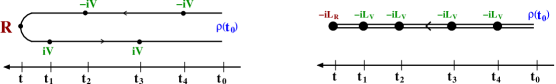
Figure 3: Expansion of the time evolution of an arbitrary observable $R$ in the coupling on the Keldysh contour (left figure) or in Liouville space (right figure), using the two different ways to write an average over an observable $R$ either in Heisenberg picture or with Liouville operators, see Eq. (68). For the Keldysh contour, operators are ordered along the contour in the direction indicated. The propagators between the vertices contain the unperturbed Hamiltonian $H_{0}$. They are given by $e^{-iH_{0}(t_{i}-t_{j})}$ for the upper branch of the Keldysh contour (forward propagation) and $e^{+iH_{0}(t_{i}-t_{j})}$ for the lower branch (backward propagation), where $t_{i}>t_{j}$ in both cases. In Liouville space all superoperators are time-ordered along one axis, the two parts of the Keldysh contour have been taken together. Correspondingly, the intermediate state in Liouville space has to be characterized by two states of the quantum system, one for the upper and one for the lower part of the Keldysh contour. For convenience, we have chosen the time direction to the left since with this convention time-ordering coincides with the sequence of Liouville operators (operators with larger time stand to the left of operators with smaller time argument).

However, instead of performing the perturbative expansion in time space, it is much easier to do it in Laplace space (at least for explicitly time-independent Hamiltonians as we are considering here). First, we define the reduced density matrix in Laplace space by

$$\tilde{\rho}_{S}(E)\,=\,\int_{t_{0}}^{\infty}dt\,e^{iE(t-t_{0})}\,\rho_{S}(t)\quad,$$ (72)

where $E$ is the Laplace variable, having a positive imaginary part to guarantee convergence. Using (67), we obtain

$$\tilde{\rho}_{S}(E)\,=\,\mbox{Tr}_{res}\,{i\over E-L}\,\rho(t_{0})\,=\,\mbox{Tr}_{res}\,{i\over E-L_{res}-L_{S}-L_{V}}\,\rho_{S}(t_{0})\rho_{res}\quad.$$ (73)

This expression can easily be expanded in $L_{V}$ by a geometric series leading to terms of the form

$$i\,\mbox{Tr}_{res}\,{1\over E-L_{res}-L_{S}}\,L_{V}\,{1\over E-L_{res}-L_{S}}\,L_{V}\,\dots\,L_{V}\,{1\over E-L_{res}-L_{S}}\,\rho_{S}(t_{0})\rho_{res}\quad.$$ (74)

The next step is to integrate out the reservoirs, i.e. the trace $\mbox{Tr}_{res}$ over the reservoir degrees of freedom has to be performed in (74). This is achieved by decomposing (74) into a product of a reservoir and system part and applying Wick’s theorem to evaluate the average over the reservoir distribution. We first exhibit explicitly all parts of the reservoir operators in (74) by finding a representation of the coupling $L_{V}$ in Liouville space similiar to the form of the coupling $V$ in Hilbert space, given by (29). We use the form

$$L_{V}\,=\,{1\over n!}\,\sigma^{p_{1}\dots p_{n}}\,G^{p_{1}\dots p_{n}}_{1\dots n}\,:J^{p_{1}}_{1}\dots J^{p_{n}}_{n}:\quad.$$ (75)

Here, $J^{p}_{1}$ are quantum field superoperators in Liouville space for the reservoirs, defined by (where $A$ is an arbitrary reservoir operator)

$$J_{1}^{p}\,A\,=\,\left\{\begin{array}[]{cl}a_{1}\,A&\mbox{for }p=+\\ A\,a_{1}&\mbox{for }p=-\end{array}\right.\quad.$$ (76)

$p$ is the Keldysh index indicating whether the field operator is acting on the upper or the lower part of the Keldysh contour. $G^{p_{1}\dots p_{n}}_{1\dots n}$ is a superoperator acting in Liouville space of the quantum system, and is defined by ($A$ is an arbitrary operator of the quantum system)

$$G^{p_{1}\dots p_{n}}_{1\dots n}\,A\,=\,\delta_{pp_{1}}\dots\delta_{pp_{n}}\,\left\{\begin{array}[]{cl}1&\mbox{for }n\mbox{ even}\\ \sigma^{p}&\mbox{for }n\mbox{ odd}\end{array}\right\}\,\left\{\begin{array}[]{cl}g_{1\dots n}\,A&\mbox{for }p=+\\ -A\,g_{1\dots n}&\mbox{for }p=-\end{array}\right.\quad.$$ (77)

We implicitly sum over $p=\pm$ on the r.h.s. of this definition, and $\sigma^{p_{1}\dots p_{n}}$ is a sign-superoperator acting in Liouville space of the quantum system, accounting for fermionic sign factors. For fermions, it is defined by its matrix representation

$$(\sigma^{p_{1}\dots p_{n}})_{ss^{\prime},\bar{s}\bar{s}^{\prime}}\,=\,\delta_{s\bar{s}}\delta_{s^{\prime}\bar{s}^{\prime}}\,\left\{\begin{array}[]{cl}p_{2}\cdot p_{4}\cdot\dots&\mbox{for }N_{s}-N_{s^{\prime}}\mbox{ even}\\ p_{1}\cdot p_{3}\cdot\dots&\mbox{for }N_{s}-N_{s^{\prime}}\mbox{ odd}\end{array}\right.\quad,$$ (78)

whereas, for bosons, it is defined by the unity operator. For $n=1$, (78) has to be interpreted as

$$(\sigma^{p})_{ss^{\prime},\bar{s}\bar{s}^{\prime}}\,=\,\delta_{s\bar{s}}\delta_{s^{\prime}\bar{s}^{\prime}}\,\left\{\begin{array}[]{cl}1&\mbox{for }N_{s}-N_{s^{\prime}}\mbox{ even}\\ p&\mbox{for }N_{s}-N_{s^{\prime}}\mbox{ odd}\end{array}\right.\quad.$$ (79)

We note some important properties of the sign operator, which will be needed later for some proofs

$$\sigma^{p_{1}\dots p_{n}p_{1}^{\prime}\dots p_{m}^{\prime}}\, = \,\sigma^{p_{1}\dots p_{n}}\,\sigma^{p_{1}^{\prime}\dots p_{m}^{\prime}}\quad\mbox{for }n\mbox{ even}\quad,$$ (80)

$$\sigma^{p_{1}\dots p_{n}}\,G^{\tilde{p}_{1}\dots\tilde{p}_{n}}_{1\dots n}\,\sigma^{p_{1}^{\prime}\dots p_{m}^{\prime}}\, = \,\sigma^{p_{1}\dots p_{n}p_{1}^{\prime}\dots p_{m}^{\prime}}\,G^{\tilde{p}_{1}\dots\tilde{p}_{n}}_{1\dots n}\quad.$$ (81)

The proof is quite easy and follows directly from the definition (78) and from the fact that, for $n$ odd, the vertex $G_{1\dots n}$ changes the parity of the particle number difference between the states on the upper and lower part of the Keldysh contour, and leaves it invariant for $n$ even, i.e. for the matrix element $(G_{1\dots n})_{ss^{\prime},\bar{s}\bar{s^{\prime}}}$ we have

$$(-1)^{N_{s}-N_{s^{\prime}}}\,=\,(-1)^{n}\,(-1)^{N_{\bar{s}}-N_{\bar{s}^{\prime}}}\quad.$$ (82)

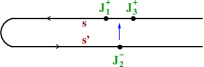
Figure 4: Determination of the fermionic sign occuring by moving the reservoir field operator $J_{2}$ from the lower to the upper part of the Keldysh contour such that the sequence $J_{1}^{+}J_{2}^{+}J_{3}^{+}\dots$ is obtained. All $J_{i}$ belong to the same coupling vertex. $s$ and $s^{\prime}$ indicate the intermediate states for the quantum system on the upper and lower part of the Keldysh contour just left to the coupling vertex.

The proof of (75) is a straightforward exercise of algebra and is provided in Appendix B. The definition of the vertex operators $G^{p_{1}\dots p_{n}}_{1\dots n}$ may at first seem unusual and it deserves some comments. It relates to the choice of the sign operators, which is in fact not unique, especially the distinction between $N_{s}-N_{s^{\prime}}$ being even or odd in (78) is not necessary (as can be seen by the proof in Appendix B, where this distinction is not used at all). However, there is a special reason why the sign operator $\sigma^{p_{1}\dots p_{n}}$ has been defined in such a way, thereby fixing the definition of the coupling vertex $G^{p_{1}\dots p_{n}}_{1\dots n}$ in Liouville space. The combination

$$\sigma^{p_{1}\dots p_{n}}\,:J^{p_{1}}_{1}\,\dots\,J^{p_{n}}_{n}:$$ (83)

has the property that the sign-operator exactly compensates additional signs due to interchanges of fermionic reservoir field operators, which arise due to the presence of field operators on the lower part of the Keldysh contour, i.e. for $p_{i}=-$. The sign from $\sigma^{p_{1}\dots p_{n}}$ is precisely the sign obtained when permuting the later operators to the corresponding position on the upper part of the Keldysh contour, assuming that all fermionic reservoir field operators anticommute. This means that the determination of the fermionic sign within Wick’s theorem (see below) can be determined as if all fermionic reservoir field operators lie on the upper part of the contour precisely in the sequence $J_{1}^{+}\dots J_{n}^{+}$ and as if the sign-operator were not present. Although there is a correction sign from the permutation of field operators belonging to the same contraction to be considered (see below), this simplifies the determination of fermionic signs considerably. To see this, consider the situation depicted in Fig. 4, where the second field operator $J_{2}^{-}$ is intended to be moved from the lower to the upper part of the Keldysh contour along the reversed direction (only virtually to determine the corresponding sign from interchanges of fermionic operators). The fermionic sign is determined by the parity of the number of fermionic reservoir field operators it passes. Up to the first field operator $J^{+}_{1}$, the parity is identical to the parity of $N_{s}-N_{s^{\prime}}$, where $s$ and $s^{\prime}$ are the intermediate states of the quantum system on the upper and lower part of the Keldysh contour left to the considered coupling vertex. The reason for this is the fact that the total parity of fermions (reservoirs plus quantum system) is conserved under the coupling and, consequently, also only those matrix elements of the reduced density matrix are unequal to zero where the parity of fermions of the quantum system are the same (in other words, the external operator $R\equiv|s\rangle\langle s^{\prime}|$ in Fig. 3 does not change the parity of fermion number). Thus, by moving $J_{2}$ finally also through $J_{1}$, we see that the parity of the total number of interchanges is odd (even) if $N_{s}-N_{s^{\prime}}$ is even (odd), which is precisely the value the sign-operator (78) produces. The same is obtained if any $J_{k}$ with $k$ even is moved virtually to the upper part of the contour, whereas for $k$ odd the total parity is identical to the parity of $N_{s}-N_{s^{\prime}}$, again corresponding to the definition (78). The same proof can be used if several $J_{k}$ are moved to the upper part, one just has to move all $J_{k}$ subsequently to the upper part, starting with the smallest $k$.

From the definitions, the following useful properties follow directly for the Liouville operators

$$\mbox{Tr}_{S}\,L_{S}\, = \,0\quad,$$ (84)

$$\sum_{p_{1}\dots p_{n}}\,\mbox{Tr}_{S}\,G^{p_{1}\dots p_{n}}_{1\dots n} = 0\quad,$$ (85)

$$\mbox{Tr}_{res}\,L_{res}\, = \,0\quad,$$ (86)

where $\mbox{Tr}_{S}$ denotes the trace with respect to the states of the quantum system. The properties (84) and (85) will turn out to be crucial for the property of conservation of probability.

Furthermore, from the (anti-)symmetry (30) of $g_{1\dots n}$ we get

$$G^{p_{1}\dots p_{i}\dots p_{j}\dots p_{n}}_{1\dots i\dots j\dots n}\,=\,\pm\,G^{p_{1}\dots p_{j}\dots p_{i}\dots p_{n}}_{1\dots j\dots i\dots n}\quad.$$ (87)

The hermiticity of the Hamiltonian $H_{S}=H_{S}^{\dagger}$ and the corresponding condition (32) for the coupling vertex imply the relations

$$(L_{S})_{ss^{\prime},\bar{s}\bar{s}^{\prime}}\, = \,-(L_{S})_{s^{\prime}s,\bar{s}^{\prime}\bar{s}}^{*}\quad,$$ (88)

$$(G^{p_{1}\dots p_{n}}_{1\dots n})_{ss^{\prime},\bar{s}\bar{s}^{\prime}}\, = \,-\,\left\{\begin{array}[]{cl}1&\mbox{for (}n\mbox{ even) or (}N_{s}-N_{s^{\prime}}\mbox{ even)}\\ -1&\mbox{for (}n\mbox{ odd) and (}N_{s}-N_{s^{\prime}}\mbox{ odd)}\end{array}\right\}\,(G^{\bar{p}_{n}\dots\bar{p}_{1}}_{\bar{n}\dots\bar{1}})_{s^{\prime}s,\bar{s}^{\prime}\bar{s}}^{*}\quad,$$ (91)

where $\bar{p}=-p$. This can be shown by some straightforward algebra. The prefactor in the last equality stems from the term $\sigma^{p}$ in the definition (77) of the coupling vertex $G$. Using the definiton (79) of $\sigma^{p}$, it can also be written in the form

$$\left\{\begin{array}[]{cl}1&\mbox{for (}n\mbox{ even) or (}N_{s}-N_{s^{\prime}}\mbox{ even)}\\ -1&\mbox{for (}n\mbox{ odd) and (}N_{s}-N_{s^{\prime}}\mbox{ odd)}\end{array}\right\}\,=\,((\sigma^{-})^{n})_{ss^{\prime},ss^{\prime}}\quad.$$ (92)

The properties (88) and (91) can be written more elegantly in operator notation by defining the c-transform $A^{c}$ for an arbitrary operator $A$ in Liouville space by

$$(A^{c})_{ss^{\prime},\bar{s}\bar{s}^{\prime}}\,=\,A_{s^{\prime}s,\bar{s}^{\prime}\bar{s}}^{*}\quad,$$ (93)

which, concerning the Keldysh contour, corresponds to interchanging the states on the upper and lower part of the contour and taking the complex conjugate (note that this definition has to be distinguished from taking the hermitian conjugate, defined by $(A^{\dagger})_{ss^{\prime},\bar{s}\bar{s}^{\prime}}=A_{\bar{s}\bar{s}^{\prime},ss^{\prime}}^{*}$). Using this formal notation together with (92), (88) and (91) can be written as

$$(L_{S})^{c}\, = \,-L_{S}\quad,$$ (94)

$$(G^{p_{1}\dots p_{n}}_{1\dots n})^{c}\, = \,-\,(\sigma^{-})^{n}\,G^{\bar{p}_{n}\dots\bar{p}_{1}}_{\bar{n}\dots\bar{1}}\quad.$$ (95)

Reversing the sequence of all indices, the last property can also be written in the form

$$(G^{p_{1}\dots p_{n}}_{1\dots n})^{c}\,=\,-\,\sigma^{--\dots-}\,G^{\bar{p}_{1}\dots\bar{p}_{n}}_{\bar{1}\dots\bar{n}}\quad,$$ (96)

where $n$ minus signs occur in the superscript of the sign operator. For the proof we used that, for $n=2r$ ($n$ even) or $n=2r+1$ ($n$ odd),

$$(\sigma^{-})^{n}\,=\,(\pm)^{r}\,\sigma^{--\dots-}$$ (97)

and (see (87))

$$G_{n\dots 1}^{p_{n}\dots p_{1}}\,=\,(\pm)^{r}\,G_{1\dots n}^{p_{1}\dots p_{n}}\quad.$$ (98)

Furthermore, for later purpose, we note the useful relations

$$(A\,B)^{c}\, = \,A^{c}\,B^{c}\quad,$$ (99)

$$(A\,a)^{\dagger}\, = \,A^{c}\,a^{\dagger}\quad,$$ (100)

where $A,B$ are superoperators and $a$ is an operator.

We turn back to the task to perform the trace over the reservoir degrees of freedom in each term (74) of perturbation theory in $L_{V}$. We insert the form (75) for all $L_{V}$ and decompose the whole expression into a product of a part for the quantum system and the reservoirs by successively moving all reservoir field operators $J_{i}^{p_{i}}$ through the resolvents to the right, starting from the last $L_{V}$. Thereby, we use the property

$$J_{1}^{p}\,L_{res}\,=\,(L_{res}-x_{1})\,J_{1}^{p}\quad,$$ (101)

where we have used the short-hand notation

$$x_{i}\,=\,\eta_{i}\,(\omega_{i}\,+\,\mu_{\alpha_{i}})\quad,$$ (102)

which will be used frequently in the following (all frequencies occur only in this combination). From (101) we get

$$:J^{p_{1}}_{1}\dots J^{p_{n}}_{n}:\,{1\over E-L_{res}-L_{S}}\,=\,{1\over E+x_{1}+\dots+x_{n}-L_{res}-L_{S}}\,:J^{p_{1}}_{1}\dots J^{p_{n}}_{n}:\quad.$$ (103)

In this way, all reservoir field operators can be moved to the right. When moving the trace $\mbox{Tr}_{res}$ in (74) to the right, we use the property (86) and can set $L_{res}\rightarrow 0$ in all resolvents. As a consequence, the term in order $r+1$ of (74) can be written symbolically in the product form

$$i\,{1\over E-L_{S}}\,({1\over n!}\sigma\,G)_{1}\,{1\over E+X_{1}-L_{S}}\,({1\over n!}\sigma\,G)_{2}\dots{1\over E+X_{r}-L_{S}}\,({1\over n!}\sigma\,G)_{r+1}\,{1\over E-L_{S}}\,\rho_{S}(t_{0})$$

$$\hskip 56.9055pt\cdot\,\langle(:J\dots J:)_{1}\,(:J\dots J:)_{2}\,\dots\,(:J\dots J:)_{r+1}\rangle_{\rho_{res}}\quad,$$ (104)

where $({1\over n!}\sigma G)_{i}$ indicates the sign and vertex operator at the $i$-th position and $(:J\dots J:)_{i}$ is the corresponding sequence of reservoir field operators. The energies $X_{i}$ are given by the sum of all $x_{k}$-variables from the field operators $J_{k}^{p_{k}}$ which occured left to the $i$-th resolvent.

The reservoir part of (104) can easily be decomposed into product of pair contractions by using Wick’s theorem. We define the following contraction for the Liouville field operators, which can easily be calculated from (27)

$$\gamma_{11^{\prime}}^{pp^{\prime}}\,=\,{J_{1}^{p}\,J_{1^{\prime}}^{p^{\prime}}\begin{picture}(-20.0,11.0)\put(-22.0,8.0){\line(0,1){3.0}} \put(-22.0,11.0){\line(1,0){12.0}} \put(-10.0,8.0){\line(0,1){3.0}} \end{picture}\begin{picture}(20.0,11.0)\end{picture}}\,\equiv\,\left\{\begin{array}[]{cl}1\\ p^{\prime}\end{array}\right\}\,\langle J_{1}^{p}J_{1^{\prime}}^{p^{\prime}}\rangle_{\rho_{res}}\,\equiv\,\left\{\begin{array}[]{cl}1\\ p^{\prime}\end{array}\right\}\,\mbox{Tr}_{res}\,J_{1}^{p}J_{1^{\prime}}^{p^{\prime}}\,\rho_{res}\,=\,\delta_{1\bar{1}^{\prime}}\,p^{\prime}\left\{\begin{array}[]{cl}\eta\\ 1\end{array}\right\}\,\,f_{\alpha}(\eta p^{\prime}\omega)\quad,$$ (105)

or

$$\gamma_{11^{\prime}}^{pp^{\prime}}\,=\,\delta_{1\bar{1}^{\prime}}\,p^{\prime}\left\{\begin{array}[]{cl}\eta\\ 1\end{array}\right\}\,\rho_{\nu}(\omega)\,f_{\alpha}(\eta p^{\prime}\omega)\quad,$$ (106)

if the density of states $\rho_{\nu}(\omega)$ is taken into the contraction according to the choice (33) and (34). The upper (lower) value corresponds as usual to bosons (fermions). Note that there is a prefactor $p^{\prime}$ for fermions in the definition of the contraction which arises as follows. As explained above the fermionic sign from the sign operators is compensated by moving all $J_{i}^{p_{i}}$ with $p_{i}=-$ to the upper part of the Keldysh contour. This means that we can use the rule that each interchange of two $J_{i}^{p_{i}}$ gives a minus sign for fermions, independent of the value of the Keldysh index $p_{i}$. However, in doing so, we do not obtain the correct sign from Wick’s theorem where it is not allowed to permute two field operators belonging to the same contraction. If we consider a contraction with $p^{\prime}=-$, we see that we permute the two field operators belonging to this contraction when moving $J_{1^{\prime}}^{-}$ to the upper part of the contour, see Fig. 5 for an illustration. Therefore, in order to get the correct sign from Wick’s theorem, we have to permute these two field operators back, leading to an additional sign for fermions. A minus sign is only obtained for fermions and $p^{\prime}=-$, leading to the prefactor $\left\{\begin{array}[]{cl}1\\ p^{\prime}\end{array}\right\}\,$ in (105).

Figure 5: Illustration why an additional fermionic sign is obtained when two field operators are contracted with the right field operator being on the lower part of the Keldysh contour (left figure). Moving $J_{1^{\prime}}$ from the lower to the upper part along the reversed direction of the contour, it passes through $J_{1}$, giving rise to an additional fermionic sign compared to the sign from Wick’s theorem. In contrast, if the right vertex lies on the upper part (right figure), the two field operators of the contraction do not pass through each other when moving $J_{1}$ to the upper part.

As a consequence, we use the following rules for the Wick decomposition

1. Contract all $J$-operators in (104) such that no contractions occur within the normal-ordered parts.

2. Disentangle the contractions into a product of pair contractions by leaving the sequence of $J$-operators within one contraction invariant. For each interchange of $J$-operators, give a minus sign for fermions.

3. Translate the contractions with (105) and sum over all possibilites to contract the field operators.

As an example, we obtain for

$$\langle:J_{1}^{p_{1}}J_{2}^{p_{2}}:\,:J_{3}^{p_{3}}J_{4}^{p_{4}}:\rangle_{\rho_{res}} = J_{1}^{p_{1}}J_{2}^{p_{2}}J_{3}^{p_{3}}J_{4}^{p_{4}}\begin{picture}(-32.0,11.0)\put(-55.0,10.0){\line(0,1){3.0}} \put(-55.0,13.0){\line(1,0){31.0}} \put(-24.0,10.0){\line(0,1){3.0}} \put(-40.0,10.0){\line(0,1){6.0}} \put(-40.0,16.0){\line(1,0){31.0}} \put(-9.0,10.0){\line(0,1){6.0}} \end{picture}\begin{picture}(32.0,11.0)\end{picture}+J_{1}^{p_{1}}J_{2}^{p_{2}}J_{3}^{p_{3}}J_{4}^{p_{4}}\begin{picture}(-32.0,11.0)\put(-55.0,10.0){\line(0,1){6.0}} \put(-55.0,16.0){\line(1,0){46.0}} \put(-9.0,10.0){\line(0,1){6.0}} \put(-40.0,10.0){\line(0,1){3.0}} \put(-40.0,13.0){\line(1,0){16.0}} \put(-24.0,10.0){\line(0,1){3.0}} \end{picture}\begin{picture}(32.0,11.0)\end{picture}$$ (107)

$$= \pm\,\gamma^{p_{1}p_{3}}_{13}\,\gamma^{p_{2}p_{4}}_{24}\,+\,\gamma^{p_{1}p_{4}}_{14}\,\gamma^{p_{2}p_{3}}_{23}\quad.$$

The corresponding diagrammatic representation is shown in Fig. 6.

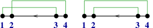
Figure 6: Diagrammatic representations of the two contributions of Eq. (107). A dot with index $i$ represents a field operator $J_{i}^{p_{i}}$. Dots standing close to each other belong to the same vertex $G$. For clarity they are separated to indicate their sequence in the original expression. This is important for the determination of the correct fermionic sign. Contractions are indicated by green lines connecting the dots. The horizontal black lines between the vertices represent the propagation of the local quantum system in Liouville space.

The energies $X_{i}$ in (104) can also be determined by a simple rule. Since the contraction (105) is only nonzero for $\eta=-\eta^{\prime}$, $\omega=\omega^{\prime}$, and $\alpha=\alpha^{\prime}$, we get $x+x^{\prime}=0$ according to the notation (102). Thus, all contractions which either stand completely to the left or to the right of the $i$-th resolvent, do not contribute to the energy $X_{i}$. Only the $x$-variables from contractions, which cross over the resolvent, contribute to $X_{i}$. Thereby, the $x$-variable has to be chosen from the $J$-operator standing left to the resolvent. This can be visualized by a simple diagrammatic rule, shown in Fig. 7. At the position of the resolvent under consideration, draw an auxiliary vertical line and consider all $x$-variables of contractions which cross this line (always taking the $x$-variable from the vertex standing left to the resolvent). The sum of all these $x$-variables is the energy $X_{i}$.

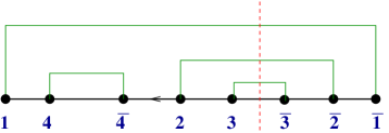
Figure 7: Rule how to calculate the energy variables of the resolvents. The energy $X$ corresponding to the resolvent standing between index $3$ and $\bar{3}$ is given by $X=x_{1}+x_{2}+x_{3}$, where $x_{i}$, $i=1,2,3$ are the variables corresponding to the contractions which cross the auxiliary vertical red line. Thereby, the $x$-variable of the field operator standing left to the resolvent has to be chosen. Note that the variable $x_{4}$ belonging to the contraction between index $4$ and $\bar{4}$ does not contribute because it does not cross the vertical cut.

Finally, we consider the determination of the prefactor, arising from the combinatorical factors ${1\over n_{i}!}$ in (104). These cancel almost completely with another factor arising from the number of identical diagrams when the $J$-operators within each normal-ordered set are permuted. The value of all these diagrams is exactly the same because the two fermionic signs arising from interchanging two reservoir field operators from the same vertex and from interchanging the two corresponding indices of the coupling vertex $G$ cancel each other, see (87). However, if $m$ contractions are present which connect the same normal-ordered blocks, there are $m!$ ways of permuting the $J$-operators of both groups in the same way without giving a new diagram. Therefore, in this case, the combinatorical factors can not be omitted completely but a symmetry factor $1/m!$ remains.

Summary of diagrammatic rules. We summarize the diagrammatic rules derived in this section to calculate the reduced density matrix of the quantum system in Laplace space. The value of a diagram is symbolically given by

$$\tilde{\rho}_{S}(E) \,\rightarrow\, {i\over S}\,(\pm)^{N_{p}}\,\left(\prod\gamma\right)\,$$ (108)

$$\cdot\,{1\over E-L_{S}}\,G\,{1\over E+X_{1}-L_{S}}\,G\,\dots\,G\,{1\over E+X_{r}-L_{S}}\,G\,{1\over E-L_{S}}\,\rho_{S}(t_{0})\quad,$$

where we use the following rules to calculate the various parts

1. $S=\prod_{i<j}m_{ij}!$ is a symmetry factor, where $m_{ij}$ is the number of contractions between vertex $i$ and $j$. Two diagrams are considered to be different if they can not be mapped on each other by permuting only the field operators of each vertex (the field operators are indicated by dots in a diagram, where dots standing close to each other belong to the same vertex).

2. $(\pm)^{N_{p}}$ is a fermionic sign factor, where $N_{p}$ is the number of interchanges of fermionic field operators $J^{p}_{i}$ in Liouville space which are needed to write the contractions in product form.

3. $\prod\gamma$ stands for the product of all contractions. If $J_{1}^{p}$ and $J_{1^{\prime}}^{p^{\prime}}$ are contracted, and $J_{1}^{p}$ stands left to $J_{1^{\prime}}^{p^{\prime}}$, the contraction is given by $\gamma^{pp^{\prime}}_{11^{\prime}}$, with (see (105))

   $$\gamma^{pp^{\prime}}_{11^{\prime}}\,=\,\delta_{1\bar{1}^{\prime}}\,p^{\prime}\left\{\begin{array}[]{cl}\eta\\ 1\end{array}\right\}\,\,f_{\alpha}(\eta p^{\prime}\omega)\quad,$$ (109)

   where $f(\omega)=1/(e^{\omega/T_{\alpha}}\mp 1)$ is the Bose (Fermi) function, and $\delta_{1\bar{1}^{\prime}}=\delta_{\eta,-\eta^{\prime}}\delta_{\nu\nu^{\prime}}\delta(\omega-\omega^{\prime})$.

4. To determine the energy argument $X_{i}$ of resolvent $i$, we draw an auxiliary vertical cut at the position of that resolvent. $X_{i}$ is the sum of all $x$-variables of the contractions which cross the vertical cut. The $x$-variable of a contraction $\gamma^{pp^{\prime}}_{11^{\prime}}$ is defined as $x=\eta(\omega+\mu_{\alpha})$, i.e. refers to the left $J_{1}^{p}$-operator of the contraction.

5. $G\equiv G^{p_{1}\dots p_{n}}_{1\dots n}$ are the coupling vertices acting on the quantum system, defined by (77). $L_{S}=[H_{S},\cdot]_{-}$ is the Liouville operator of the quantum system.

6. The formal indices $1\equiv\eta\nu\omega$ and $\nu\equiv\alpha\sigma\dots$ contain the index $\eta=\pm$ for creation/annihilation operators, the energy $\omega$ of the reservoir state (relative to the chemical potential $\mu_{\alpha}$), the reservoir index $\alpha$, the spin index $\sigma$, and possible other quantum numbers characterizing the reservoir state. We sum (integrate) over all these indices implicitly.

To write the resolvents in a compact way, we use the short-hand notation

$$\Pi_{12\dots n}\,\equiv\,{1\over E+x_{1}+x_{2}+\dots x_{n}-L_{S}}\quad.$$ (110)

With this convention, the diagram example of Fig. 8 is given by

$${i\over 2}\,(\pm)\,\gamma_{17}\,\gamma_{23}\,\gamma_{4,12}\,\gamma_{56}\,\gamma_{8,11}\,\gamma_{9,10}$$ (111)

$$\cdot\,{1\over E-L_{S}}\,G_{12}\,\Pi_{12}\,G_{345}\,\Pi_{145}\,G_{6789}\,\Pi_{489}\,G_{10,11,12}\,{1\over E-L_{S}}\,\rho_{S}(t_{0})\quad,$$

where we have omitted for simplicity the obvious Keldysh indices at the couping vertices $G$ and the contractions $\gamma$. The factor ${1\over 2}$ arises from the fact that the third and fourth vertex are connected by two contractions, and the sign factor $\pm$ stems from taking the contraction $\gamma_{4,12}$ out of the rest.

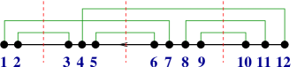
Figure 8: Example of a diagram with four vertices. The vertical cuts are auxiliary lines between the vertices to determine the indices of the resolvents $\Pi_{\dots}$ in (111). Precisely those indices occur which belong to the left field operator of each contraction crossing the vertical cut.

Kinetic equation. The diagrammatic expansion can be formally resummed and written in the form of a kinetic equation by distinguishing between irreducible and reducible diagrams. Irreducible diagrams are those diagrams where any vertical cut hits at least one reservoir contraction, i.e. in each resolvent at least one $x$-variable occurs. In contrast, in reducible diagrams there are vertical cuts crossing no contraction, corresponding to a resolvent of the form $1/(E-L_{S})$ without any $x$-variable, see Fig. 9 for illustration.

Figure 9: Irreducible (left) and reducible (right) diagrams. In the left figure any vertical cut between the vertices hits at least one reservoir contraction. In the right figure, the vertical cut between the second and third vertex does not hit any contraction and corresponds to a resolvent of the form ${1\over E-L_{S}}$.

We denote the sum over all irreducible diagrams by the irreducible kernel $\Sigma(E)$. Using (108), we obtain the following value for any diagram of the kernel

$$\Sigma(E)\,\rightarrow\,{1\over S}\,(\pm)^{N_{p}}\,\left(\prod\gamma\right)_{irr}\,G\,{1\over E+X_{1}-L_{S}}\,G\,\dots\,G\,{1\over E+X_{r}-L_{S}}\,G\quad,$$ (112)

where $(\prod\gamma)_{irr}$ means that we only consider irreducible diagrams. Compared to (108), we have omitted in this definition the prefactor $i$, the first and last resolvent, and the initial density matrix $\rho_{S}(t_{0})$.

Each diagram for $\tilde{\rho}_{S}(E)$ can be written as a sequence of irreducible parts with resolvents $1/(E-L_{S})$ in between. Similiar to Dyson equations within Green’s function methods, all irreducible diagrams can be formally resummed to define the kernel $\Sigma(E)$, and the total sum of all diagrams can be written as a geometric series

$$\tilde{\rho}_{S}(E)\,=\,i\,{1\over E-L_{S}}\,\sum_{n=0}^{\infty}\,\left(\Sigma(E){1\over E-L_{S}}\right)^{n}\,\rho_{S}(t_{0})\,=\,{i\over E-L_{S}-\Sigma(E)}\,\rho_{S}(t_{0})\quad,$$ (113)

leading to the final result

$$\tilde{\rho}_{S}(E)\,=\,{i\over E-L_{S}^{eff}(E)}\,\rho_{S}(t_{0})\quad,$$ (114)

where

$$L_{S}^{eff}(E)\,=\,L_{S}\,+\,\Sigma(E)$$ (115)

is an effective Liouville operator of the quantum system, which depends on the Laplace variable $E$. From (85) and the fact that any diagram for $\Sigma(E)$ starts with a coupling vertex $G$, we get the important property

$$\mbox{Tr}_{S}\,\Sigma(E)\,=\,\mbox{Tr}_{S}\,L_{S}^{eff}(E)\,=\,0\quad,$$ (116)

which is important for conservation of probability (see below). Furthermore, in analogy to (94), we have

$$(L_{S}^{eff}(E))^{c}\,=\,-L_{S}^{eff}(-E^{*})\quad,\quad(\Sigma(E))^{c}\,=\,-\Sigma(-E^{*})\quad.$$ (117)

The proof of this relation is provided in Appendix C.

Eq. (114) is the central result of this section. It shows very clearly the effect of the coupling to the reservoirs. In the absence of a coupling to the reservoirs, the kernel $\Sigma(E)$ is zero, and $L_{S}^{eff}$ is identical to the bare Liouvillian $L_{S}$, which is hermitian. As a consequence, the poles of $\tilde{\rho}_{S}(E)$ lie on the real axis, corresponding to coherent Rabi oscillations of the quantum system in time space. In contrast, when the coupling to the reservoirs is nonzero, a dissipative part $\Sigma(E)$ has to be added to the effective Liouvillian and the analytic structure of the reduced density matrix changes in Laplace space as illustrated in Fig. 10. Generically, a branch cut will occur on the real axis due to the continuous spectrum of the reservoirs. Analogous to the theory of quantum decay, we turn this branch cut into the lower half of the complex plane by analytic continuation. This leads to poles in the lower half plane, which originally were on the real axis in the absence of the coupling to the reservoirs. These poles correspond to exponential decay, the negative imaginary part is the decay rate $\Gamma$ (relaxation or dephasing rate, depending on whether the mode corresponds to decay of diagonal or nondiagonal matrix elements of the reduced density matrix of the quantum system), and the real part corresponds to the oscillation frequency $h$ (e.g. an effective magnetic field). The remaining branch cuts can e.g. lead to power law decay, but usually their prefactor is smaller than the one of the exponential decay modes, and they dominate only the long-time behaviour. Generically, there will be always a single pole at $E=0$, which corresponds to the stationary state (for certain symmetries or in the case of symmetry breaking, it may not be unique accidentally). It is determined by the eigenvalue equation

$$L_{S}^{eff}(i0^{+})\,\rho_{S}^{st}\,=\,0\quad.$$ (118)

This pole will play an essential role within the RG formalism presented in Sec. 4, since it does not decay. It will be shown that it can be included perturbatively into the initial condition of effective vertices, whereas the decay rates $\Gamma_{i}$ and the oscillation frequencies $h_{i}$ provide the cutoff of the RG flow. An important advantage of the present formalism is that the physical decay rates, determining the time evolution of the reduced density matrix of the quantum system, follow directly from the poles of Eq. (114). Once the kernel $\Sigma(E)$ has been calculated within perturbation theory (using the diagrammatic rules (112)) or even nonperturbatively using the RTRG-FS scheme set up in Sec. 4, the decay modes can easily be found. In contrast, within slave particle formalism, the physical decay rates have to be calculated in a complicated way by combining self-energy insertions and vertex corrections paaske_rosch_kroha_woelfle_PRB04 , and within flow-equation methods the decay rates follow from the energy scale where certain 1-loop and 2-loop contributions become of equal order on the r.h.s. of the flow equations.

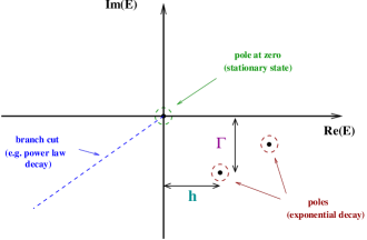
Figure 10: Analytic properties of $\tilde{\rho}_{S}(E)$. Poles occur in the lower half plane leading to exponential decay. $\Gamma$ denotes the relaxation or dephasing rate, $h$ is the oscillation frequency. The pole at $E=0$ is always present and unique, it corresponds to the stationary state. Generically, branch cuts will also occur, leading e.g. to power law decay.

Conservation of probability follows from (116). Acting with the trace $\mbox{Tr}_{S}$ over the quantum system on Eq. (114), we obtain

$$\mbox{Tr}_{S}\,\tilde{\rho}_{S}(E)\,=\,{i\over E}\,\mbox{Tr}_{S}\,\rho_{S}(t_{0})\quad,$$ (119)

which, after transforming back to time space, gives

$$\mbox{Tr}_{S}\,\rho_{S}(t)\,=\,\mbox{Tr}_{S}\,\rho_{S}(t_{0})\quad,$$ (120)

i.e. the normalization of the reduced density matrix is invariant and stays unity if it is normalized initially $\mbox{Tr}_{S}\rho(t_{0})=1$. Note that this property holds within any diagrammatic approximation, because any diagram for the kernel $\Sigma(E)$ starts with a coupling vertex $G$. We will also see in Sec. 4 that the RG flow within RTRG-FS preserves conservation of probability in any approximation scheme.

Furthermore, by applying the property (100) to (114), we can show from (117) and $\rho_{S}(t_{0})^{\dagger}=\rho_{S}(t_{0})$ that $\tilde{\rho}_{S}(E)$ fulfils the condition

$$\tilde{\rho}_{S}(E)^{\dagger}\,=\,\tilde{\rho}_{S}(-E^{*})\quad,$$ (121)

which is equivalent to the hermiticity of the reduced density matrix in time space

$$\rho_{S}(t)^{\dagger}\,=\,\rho_{S}(t)\quad.$$ (122)

Eq. (114) can also be written in time space leading to a kinetic equation. Multiplying Eq. (114) with $-i(E-L_{S}-\Sigma(E))$, we obtain

$$\left[-i\,E\,\tilde{\rho}_{S}(E)\,-\,\rho_{S}(t_{0})\right]\,+\,i\,L_{S}\,\tilde{\rho}_{S}(E)\,=\,-i\,\Sigma(E)\,\tilde{\rho}_{S}(E)\quad.$$ (123)

Using (72) and the definition

$$\Sigma(E)\,=\,\int_{0}^{\infty}dt\,e^{iEt}\,\Sigma(t)$$ (124)

for the kernel in time space, we see that (123) is equivalent to the following kinetic equation in time space

$${d\over dt}\,\rho_{S}(t)\,+\,i\,L_{S}\,\rho_{S}(t)\,=\,-i\,\int_{t_{0}}^{t}dt^{\prime}\,\Sigma(t-t^{\prime})\,\rho_{S}(t^{\prime})\quad.$$ (125)

The second term on the l.h.s. corresponds to the von Neumann equation of the isolated quantum system, whereas the r.h.s. describes the non-Markovian dissipative influence of the coupling to the reservoirs.

Kinetic equations of the form (125) are not new in dissipative quantum mechanics and can also be derived by other methods, e.g. with projection operators zwanzig or within slave particle techniques rosch_paaske_kroha_woelfle_PRL03 . However, the crucial point is not the form of the kinetic equation (which is trivial and obvious on physical grounds) but the way the kernel $\Sigma$ is calculated. Using projection operator techniques a purely formal but quite compact expression of the kernel is obtained where certain projectors $Q=1-P$, with $P=\rho_{res}\mbox{Tr}_{res}$, occur between the Liouville operators $L_{V}$ projecting on the irreducible part. However, this does not help at all for the calculation of $\Sigma$ because the reservoir degrees of freedom are still present in $L_{V}$. Only after the insertion of $Q=1-P$, an explicit calculation can be started but an artificial decomposition into reducible parts is created, induced by the projection operator $P$. All the reducible terms finally cancel in a complicated way, leaving only those terms of the Wick decomposition which are irreducible. In contrast, the diagrammatic rule (112) derived in this section considers directly the irreducible terms, and the reservoir degrees of freedom are already integrated out. Using slave-particle techniques and Keldysh-formalism, the derivation of a kinetic equation (or quantum Boltzmann equation) is quite complicated (even in lowest order perturbation theory), and the kernel $\Sigma$ is a complicated mixture of self-energy contributions and vertex corrections. Therefore, we believe that the calculation of the kernel via the diagrammatic rule (112) is very efficient. This has been demonstrated recently within perturbation theory up to fourth order in the coupling vertex for problems of molecular electronics leinjse_wegewijs . In Sec. 4 we will see that it is especially useful for setting up nonequilibrium RG methods which incorporate the physics of relaxation and dephasing.

3.2 Observables

Observables. The time evolution of an arbitrary observable $R$ can be calculated starting from Eqs. (68) and (69)

$$\langle R\rangle(t)\,=\,\mbox{Tr}_{S}\,\mbox{Tr}_{res}\,(-iL_{R})e^{-iL(t-t_{0})}\,\rho_{S}(t_{0})\rho_{res}\quad,\quad L_{R}\,=\,{i\over 2}\,[R,\cdot]_{+}\quad.$$ (126)

The observable $R$ is written in the same generic form (29) as the coupling $V$

$$R\,=\,{1\over n!}\,r_{1\dots n}\,:a_{1}\dots a_{n}:\quad,$$ (127)

with $n=0,1,2,\dots$ (in contrast to $V$, where the $n=0$ case can be incorporated in $H_{S}$, this is not possible for $R$). Due to (anti-)symmetry and hermiticity, we get similiar to (30) and (32) the properties

$$r_{1\dots i\dots j\dots n}\, = \,\pm\,r_{1\dots j\dots i\dots n}\quad,$$ (128)

$$(r_{12\dots n})^{\dagger}\, = \,r_{\bar{n}\dots\bar{1}}\quad.$$ (129)

Analogous to (75), we obtain a corresponding form for the operator $L_{R}$ in Liouville space

$$L_{R}\,=\,{1\over n!}\,\sigma^{p_{1}\dots p_{n}}\,R^{p_{1}\dots p_{n}}_{1\dots n}\,:J^{p_{1}}_{1}\dots J^{p_{n}}_{n}:\quad,$$ (130)

with the vertex of the observable given by

$$R^{p_{1}\dots p_{n}}_{1\dots n}\,A\,=\,{i\over 2}\,\delta_{pp_{1}}\dots\delta_{pp_{n}}\,\left\{\begin{array}[]{cl}1&\mbox{for }n\mbox{ even}\\ \sigma^{p}&\mbox{for }n\mbox{ odd}\end{array}\right\}\,\left\{\begin{array}[]{cl}r_{1\dots n}\,A&\mbox{for }p=+\\ A\,r_{1\dots n}&\mbox{for }p=-\end{array}\right.\quad.$$ (131)

The difference to (77) stems from the form $L_{R}={i\over 2}[R,\cdot]_{+}$ where the anticommutator and a different prefactor occurs in comparism to $L_{V}=[V,\cdot]_{-}$. The prefactor $i/2$ is taken into the definition of the vertex $R$ to get diagrammatic rules similiar to the ones for the reduced density matrix and the kernel $\Sigma$ (see below). We note that the trace over the states of the quantum system always occurs left to $L_{R}$ in the average (126), i.e. we get

$$\mbox{Tr}_{S}\,L_{R}\dots\,=\,\sum_{s}\,(L_{R})_{ss,\cdot\cdot}\dots\quad.$$ (132)

Therefore, according to the definition (79), the sign operator $\sigma^{p}$ can be dropped in (131) for the calculation of $\langle R\rangle(t)$, and $\sigma^{p_{1}\dots p_{n}}$ can be replaced by

$$\sigma^{p_{1}\dots p_{n}}\,\rightarrow\,p_{2}p_{4}\dots\quad.$$ (133)

Nevertheless, for the formal identity (131) the sign operators have to be used in their general form.

Similiar to (95), one can easily show from the definition (131) and the hermiticity condition (129) the relation

$$(R^{p_{1}\dots p_{n}}_{1\dots n})^{c}\,=\,-\,(\sigma^{-})^{n}\,R^{\bar{p}_{n}\dots\bar{p}_{1}}_{\bar{n}\dots\bar{1}}\quad.$$ (134)

In Laplace space we obtain from (126)

$$\tilde{\langle R\rangle}(E)\,=\,\int_{t_{0}}^{\infty}dt\,e^{iE(t-t_{0})}\,\langle R\rangle(t)\,=\,\mbox{Tr}_{S}\,\mbox{Tr}_{res}\,L_{R}\,{1\over E-L_{res}-L_{S}-L_{V}}\,\rho_{S}(t_{0})\rho_{res}\quad,$$ (135)

which, after expanding in $L_{V}$, leads to terms of the form

$$\mbox{Tr}_{S}\,\mbox{Tr}_{res}\,L_{R}\,{1\over E-L_{res}-L_{S}}\,L_{V}\,{1\over E-L_{res}-L_{S}}\,L_{V}\,\dots\,L_{V}\,{1\over E-L_{res}-L_{S}}\,\rho_{S}(t_{0})\rho_{res}\quad.$$ (136)

The trace over the reservoirs can be evaluated in the same way as described in Sec. 3.1 for (74), and we obtain for a certain diagram of the average of an observable in analogy to (108)

$$\tilde{\langle R\rangle}(E) \,\rightarrow\, {1\over S}\,(\pm)^{N_{p}}\,\left(\prod\gamma\right)\,$$ (137)

$$\cdot\,\mbox{Tr}_{S}\,R\,{1\over E+X_{1}-L_{S}}\,G\,{1\over E+X_{2}-L_{S}}\,\dots\,G\,{1\over E+X_{r}-L_{S}}\,G\,{1\over E-L_{S}}\,\rho_{S}(t_{0})\quad$$

with the essential difference that the first vertex corresponds to the vertex of the observable $R$ and the trace $\mbox{Tr}_{S}$ over the quantum system has to be performed.

Decomposing (137) into reducible and irreducible parts and resumming formally all diagrams leads to

$$\tilde{\langle R\rangle}(E)\,=\,\mbox{Tr}_{S}\,\Sigma_{R}(E)\,{1\over E-L_{S}^{eff}(E)}\,\rho_{S}(t_{0})\,=\,-i\,\mbox{Tr}_{S}\,\Sigma_{R}(E)\,\tilde{\rho}_{S}(E)\quad,$$ (138)

where we have used (114) in the last equality. Here, the kernel $\Sigma_{R}(E)$ is defined analogous to $\Sigma(E)$ with the only difference that the first vertex is replaced by the observable vertex $R$, i.e. in analogy to (112) the observable kernel $\Sigma_{R}(E)$ is given by the diagrams

$$\Sigma_{R}(E)\,\rightarrow\,{1\over S}\,(\pm)^{N_{p}}\,\left(\prod\gamma\right)_{irr}\,R\,{1\over E+X_{1}-L_{S}}\,G\,\dots\,G\,{1\over E+X_{r}-L_{S}}\,G\quad.$$ (139)

Eqs. (138) and (139) are the final result for the average of an observable. Once the kernels $\Sigma_{R}(E)$ and $\Sigma(E)$ have been calculated, they can be inserted into Eq. (138) and the average of an observable can be calculated for all values of the Laplace variable $E$, i.e. the full time evolution can be obtained by transforming to time space. The stationary value of the average of an observable is given by

$$\langle R\rangle^{st}\,=\,\lim_{t\rightarrow\infty}\langle R\rangle(t)\,=\,-i\lim_{E\rightarrow i0^{+}}E\,\tilde{\langle R\rangle}(E)\quad,$$ (140)

which, using (138), gives

$$\langle R\rangle^{st}\,=\,-i\,\mbox{Tr}_{S}\,\Sigma_{R}(i0^{+})\,\rho_{S}^{st}\quad,$$ (141)

where $\rho_{S}^{st}$ is the stationary value of the reduced density matrix of the quantum system, which can be calculated from $L_{S}^{eff}(i0^{+})\rho_{S}^{st}=0$, see (118).

Finally, we note that similiar to (117), one can prove

$$(\Sigma_{R}(E))^{c}\,=\,-\Sigma_{R}(-E^{*})\quad,$$ (142)

which, together with the hermiticity condition (121) for the reduced density matrix, proves that (138) respects the hermiticity of the observable $R$

$$\langle\tilde{R}\rangle(E)^{*}\,=\,\tilde{\langle R\rangle}(-E^{*})\quad,$$ (143)

implying that $\langle R\rangle(t)$ is real in time space.

An important example of an observable is the particle current operator $I^{\gamma}$ flowing from reservoir $\gamma$ to the quantum system (for electrons, the charge current is obtained by multiplying with $-e$). It is defined by

$$I^{\gamma}\,=\,-{d\over dt}N_{res}^{\gamma}\quad,$$ (144)

where $N_{res}^{\gamma}$ is the particle number operator for reservoir $\gamma$ and the derivative is calculated via the Heisenberg picture for the Hamiltonian (13)

$$I^{\gamma}\, = \,-i\,[H,N^{\gamma}_{res}]\,=\,-i\,[V,N^{\gamma}_{res}]\,=\,$$ (145)

$$= \,-i\,{1\over n!}\,g_{1\dots n}\,[:a_{1}\dots a_{n}:,N^{\gamma}_{res}]$$

$$= \,{1\over n!}\,i\sum_{i=1}^{n}\,\eta_{i}\,\delta_{\alpha_{i}\gamma}\,g_{1\dots n}\,:a_{1}\dots a_{n}:\quad,$$

where the form (29) for $V$ has been inserted, and we used the identity $[a_{1},N_{res}^{\gamma}]=-\eta\delta_{\alpha\gamma}a_{1}$ in the last step. Note that we mean by the time derivative ${d\over dt}N_{res}^{\gamma}$ of the particle number in reservoir $\gamma$ not the total time derivative, including the one from the coupling of the reservoir to the bath maintaining the temperature $T_{\gamma}$ and the chemical potential $\mu_{\gamma}$ of the reservoir (leading to the grandcanonical distribution for reservoir $\gamma$). This total time derivative would be zero on average since the average particle number in the reservoir is a constant. Therefore, to get a definition of the local current operator at the position where the reservoir is coupled to the quantum system, we include in the time derivative only the term $i[V,N_{res}]$ due to the coupling between reservoir and quantum system.

In summary, the current operator can be brought into the form (127)

$$I^{\gamma}\,=\,{1\over n!}\,i^{\gamma}_{1\dots n}\,:a_{1}\dots a_{n}:\quad,$$ (146)

with

$$i^{\gamma}_{1\dots n}\,=\,i\,\sum_{i=1}^{n}\,\eta_{i}\,\delta_{\alpha_{i}\gamma}g_{1\dots n}\quad.$$ (147)

Inserting this form of $i^{\gamma}_{1\dots n}$ into (131) for $r_{1\dots n}$, and using (77), we obtain from (130) for the current operator in Liouville space

$$L_{I^{\gamma}}\,=\,{1\over n!}\,\sigma^{p_{1}\dots p_{n}}\,(I^{\gamma})^{p_{1}\dots p_{n}}_{1\dots n}\,:J^{p_{1}}_{1}\dots J^{p_{n}}_{n}:\quad,$$ (148)

with

$$(I^{\gamma})^{p_{1}\dots p_{n}}_{1\dots n}\,=\,-{1\over 2}\,\sum_{i=1}^{n}\,\eta_{i}\delta_{\alpha_{i}\gamma}\,\delta_{p_{1}p}\dots\delta_{p_{n}p}\,p\,G^{p\dots p}_{1\dots n}\quad.$$ (149)

4 Nonequilibrium RG in Liouville space

In this section we develop a nonequilibrium renormalization group method based on the diagrammatic rules derived in the previous section. It is a formally exact RG-approach in the sense that an infinite hierarchy of RG equations will be set up, which, if solved completely, would provide the full solution of the problem. Of course , in practice, approximations in form of truncation schemes have to be used. Nevertheless, it is quite useful to know what terms have been neglected in order to be able to improve the calculations systematically. Formally exact RG approaches are used in many fields of physics at the moment and are based on different ideas. The most conventional one is to integrate out energy (or momentum) scales step by step (starting from high energies) and leaving the whole set of diagrams invariant by renormalizing certain parameters, based on the pioneering ideas of Wilson rg_wilson . This basic idea will be also the guideline of our RG procedure, although the way we define the cutoff function is quite different. Furthermore, our diagrammatic language is more complicated since the vertices are still operators on the local quantum system and their time-ordering has to be considered. As a consequence, we have to use the Laplace transform (instead of the usual Fourier transform) and renormalization group will generate an additional energy dependence $L_{S}(E)$ and $G_{1\dots n}^{p_{1}\dots p_{n}}(E)$ of the Liouvillian and the vertices, which can only be described within a diagrammatic representation (in contrast to approaches based on projection operators). This energy will turn out to be the equivalent of the Laplace variable, opening the possibility to address the full time-evolution of the problem (however, also for the calculation of the stationary state, the additional energy dependence has to be taken into account in the RG equations). We will formulate the RG approach such that all vertices stay in normal-ordered form but it can also be formulated without normal-ordering. In standard quantum field theory (where all degrees of freedom are integrated out and the vertices are c-numbers), similiar RG approaches have been developed based on the same idea, see the normal-ordered version by Salmhofer salmhofer and the non normal-ordered version by Polchinski polchinski (usually the RG equations are derived within path integral formalism but they can also be obtained on a pure diagrammatic level using the idea of invariance hs_private ). In this sense, the RG method presented in this section is a generalization to nonequilibrium and to the case where the vertices are operators. Furthermore, we note that using the Laplace transform has the consequence that no energy conservation is associated with the vertices but, as we will see, it has the advantage that the structure of the Keldysh indices becomes very simple. We will show that by integrating out the symmetric part of the reservoir distribution from the very beginning, the final RG equations do not contain Keldysh indices at all. This simplifies the calculations considerably. Furthermore, we will see that the physical relaxation and dephasing rates (describing the rates associated with quantum transport and not with quantum decay or single-particle life times as in usual Green’s function methods) occur quite natural and can be incorporated directly into the RG equations. Therefore, our RG schemes seems to be an appropriate way to combine RG with the physics of relaxation and dephasing, an important subject in mesoscopics, quantum information processing and cold atom systems.

We mention that there are other formally exact RG approaches in quantum field theory which do not use the conventional idea of integrating out energy degrees of freedom and leaving the sum of all diagrams invariant by renormalization. One of them is the RG developed by Wetterich wetterich where cutoff dependent 1-particle irreducible vertex function are defined, such that the initial condition at cutoff $\Lambda=\infty$ gives the bare vertices whereas for $\Lambda=0$ the full physical vertex functions are obtained. Differential equations are then set up directly for these vertex functions from which they can be calculated systematically using appropriate truncation schemes. This scheme is specifically adapted to the conventional diagrammatic representation of quantum field theories and, therefore, can not be overtaken directly to the diagrammatic language used in this paper. The concept of irreducibility is defined completely different here and the diagrams generated by our RG procedure are automatically irreducible. Within the RTRG-FS approach the irreducible diagrams, represented by the kernel $\Sigma(E)$, are fed back into the RG equations for the vertices via an effective description of the dynamics of the local quantum system. This is analogous to the Wetterich RG scheme where the propagators include self-energy insertions. For problems where a controlled expansion in the Coulomb interaction is possible, the Wetterich RG method is very powerful and, recently, has also been generalized to the nonequilibrium case jakobs_diplom ; jakobs_meden_hs_PRL07 ; gezzi_pruschke_meden_PRB07 . Another RG method is the flow equation method developed by Glazek, Wegner, and Wilson flow_eq , which recently has been generalized to the nonequilibrium and time-dependent case by Kehrein et al. kehrein_PRL05 ; moeckel_kehrein_PRL08 . This scheme is based on a pure Hamiltonian level and the Hamiltonian is diagonalized by unitary transformations step by step. This idea is competely different from all other formally exact RG methods and can be viewed as a technical alternative to the scheme presented here.

4.1 Basic ideas and cutoff function

The central quantities of interest are the effective Liouvillian $L_{S}^{eff}(E)$ (or equivalently the irreducible kernel $\Sigma(E)$) and the kernel $\Sigma_{R}(E)$, given by the diagrammatic representation (see (112) and (139))

$$\left\{\begin{array}[]{cl}L_{S}^{eff}(E)\\ \Sigma_{R}(E)\end{array}\right\}\,\rightarrow\,\left\{\begin{array}[]{cl}L_{S}\\ R_{n=0}\end{array}\right\}+{1\over S}(\pm)^{N_{p}}\left(\prod\gamma\right)_{irr}\left\{\begin{array}[]{cl}G\\ R\end{array}\right\}{1\over E+X_{1}-L_{S}}G\dots G{1\over E+X_{r}-L_{S}}G\,.$$ (150)

The first term represents the $n=0$ case and is written explicitly because $G_{n=0}$ is by convention incorporated in $L_{S}$. The second term represents all diagrams with more than one vertex or, equivalently, with at least one reservoir contraction. There, the difference is only the first vertex, which is $G$ for $L_{S}^{eff}(E)$ and $R$ for $\Sigma_{R}(E)$. From these quantities the reduced density matrix and the average of the observable $R$ can be calculated by using (114) and (138)

$$\tilde{\rho}_{S}(E)\,=\,{i\over E-L_{S}^{eff}(E)}\,\rho_{S}(t_{0})\quad,\quad\tilde{\langle R\rangle}(E)\,=\,-i\,\mbox{Tr}_{S}\,\Sigma_{R}(E)\,\tilde{\rho}_{S}(E)\quad,$$ (151)

and the irreducible kernel $\Sigma(E)$ can be obtained from

$$L_{S}^{eff}(E)\,=\,L_{S}\,+\,\Sigma(E)\quad.$$ (152)

To find a mathematically well-defined formulation of renormalization group (RG), we note that the physical quantities of interest are a functional of the reservoir contraction $\gamma$, the vertices $G$ and $R$, and the Liouvillian $L_{S}$

$$L_{S}^{eff}(E)\, = \,L_{S}\,+\,{\cal{F}}(\gamma,L_{S},G)\quad,$$ (153)

$$\Sigma_{R}(E)\, = \,R_{n=0}\,+\,{\cal{F}}_{R}(\gamma,L_{S},G,R)\quad.$$ (154)

The functionals $\cal{F}$ and $\cal{F}_{R}$ represent the diagrammatic rules of the second term of Eq. (150). Note that the $n=0$ case is written explicitly in the first term, so that the arguments of the functionals do not include the case $n=0$ for the vertices $G_{1\dots n}$ and $R_{1\dots n}$.

The idea of RG is to integrate out the reservoir degrees of freedom and to account for these by a renormalization of the system parameters without changing the diagrammatic rules. This leads to an effective theory for the dynamics of the local quantum system. To achieve this, we replace the reservoir correlation function $\gamma$ in the functionals (153) and (154) by a cutoff dependent contraction $\gamma^{\Lambda}$, and try to find a corresponding $\Lambda$-dependence of the Liouvillian $L_{S}\rightarrow L_{S}^{\Lambda}$ and the vertices $G,R\rightarrow G^{\Lambda},R^{\Lambda}$, such that, without changing the diagrammatic rules (i.e. the functionals), the sum of all diagrams stays invariant, which gives

$$L_{S}^{eff}(E)\, = \,L_{S}^{\Lambda}(E)\,+\,{\cal{F}}(\gamma^{\Lambda},L_{S}^{\Lambda},G^{\Lambda})\quad,$$ (155)

$$\Sigma_{R}(E)\, = \,R_{n=0}^{\Lambda}(E)\,+\,{\cal{F}}_{R}(\gamma^{\Lambda},L_{S}^{\Lambda},G^{\Lambda},R^{\Lambda})\quad.$$ (156)

This is the important property of invariance since the r.h.s. gives always the same independent of $\Lambda$. In this way an effective theory can be formulated where both the reservoirs and the quantum system are modified, but the physics of the total system stays invariant (in principle also the functionals $\cal{F}$ and $\cal{F}_{R}$ can be replaced by a cutoff-dependent functional but we will not consider this case here). However, as we will see in Sec. 4.2, invariance can only be maintained if the Liouvillian and the vertices get an additional energy dependence

$$L_{S}\, \rightarrow \,L_{S}^{\Lambda}(E)\quad,\quad$$ (157)

$$G^{p_{1}\dots p_{n}}_{1\dots n}\, \rightarrow \,(G^{\Lambda})^{p_{1}\dots p_{n}}_{1\dots n}(E)\quad,\quad$$ (158)

$$R^{p_{1}\dots p_{n}}_{1\dots n}\, \rightarrow \,(R^{\Lambda})^{p_{1}\dots p_{n}}_{1\dots n}(E)\quad,\quad$$ (159)

and a new diagrammatic rule has to be set up which states that the energy argument $E+X_{i}$ occuring in some resolvent of (150) is the same for the Liouvillian occuring in that resolvent and for the vertex to the right of that resolvent (the first vertex gets the energy argument $E$), i.e. (150) has to be replaced by

$$\left\{\begin{array}[]{cl}L_{S}^{eff}(E)\\ \Sigma_{R}(E)\end{array}\right\}\, \rightarrow \,\left\{\begin{array}[]{cl}L_{S}^{\Lambda}(E)\\ R^{\Lambda}_{n=0}(E)\end{array}\right\}\,+\,{1\over S}\,(\pm)^{N_{p}}\,\left(\prod\gamma^{\Lambda}\right)_{irr}\left\{\begin{array}[]{cl}G^{\Lambda}(E)\\ R^{\Lambda}(E)\end{array}\right\}$$

$$\cdot\,{1\over E+X_{1}-L_{S}^{\Lambda}(E+X_{1})}\,G^{\Lambda}(E+X_{1})\,\dots\,{1\over E+X_{r}-L_{S}^{\Lambda}(E+X_{r})}\,G^{\Lambda}(E+X_{r})\quad.$$

The advantage of this formally exact scheme is that one can choose the value for the parameter $\Lambda$ and the way one defines the $\Lambda$-dependence of the reservoir contraction $\gamma^{\Lambda}$ in an arbitrary way, opening up many possibilities for RG schemes. However, only those schemes are of course of practical use, where the $\Lambda$-dependence of the Liouvillian and the vertices can be found in a systematic way, and where the final evaluation of (4.1) for a certain value of $\Lambda$ has some advantage compared to the original series (150). We discuss some of these schemes in the following.

Continuous RG scheme. If the parameter $\Lambda$ is a continuous parameter with initial value $\Lambda_{in}$ and final value $\Lambda_{fi}$, one defines the boundary conditions of the contraction such that

$$\gamma^{\Lambda_{in}}\,=\,\gamma\quad,\quad\gamma^{\Lambda_{fi}}\,=\,0\quad,$$ (167)

i.e. the initial contraction is the original reservoir correlation function and the final one is defined as zero. As a consequence the initial values of the Liouvillian and the vertices are the original ones

$$L_{S}^{\Lambda_{in}}(E)\, = \,L_{S}\quad,\quad$$ (168)

$$(G^{\Lambda_{in}})^{p_{1}\dots p_{n}}_{1\dots n}(E)\, = \,G^{p_{1}\dots p_{n}}_{1\dots n}\quad,\quad$$ (169)

$$(R^{\Lambda_{in}})^{p_{1}\dots p_{n}}_{1\dots n}(E)\, = \,R^{p_{1}\dots p_{n}}_{1\dots n}\quad,$$ (170)

such that the original perturbative expansion (150) is reproduced. For the final value $\Lambda=\Lambda_{fi}$, the reservoir contraction is zero, and only the diagrams of (4.1) survive where no contractions are present, i.e. the $n=0$ vertices, represented by $L_{S}^{\Lambda}(E)$ and $R^{\Lambda}_{n=0}(E)$. Thus, the result for the physical quantities is given by

$$L_{S}^{eff}(E)\,=\,L^{\Lambda_{fi}}_{S}(E)\quad,\quad\Sigma_{R}(E)\,=\,R^{\Lambda_{fi}}_{n=0}(E)\quad.$$ (171)

We see that $L_{S}^{\Lambda}(E)$ and $R^{\Lambda}_{n=0}(E)$ flow finally into the physical quantities and, therefore, we interpret them as effective physical quantities at scale $\Lambda$. If $\Lambda$ is an energy cutting off the high-energy scales of the reservoirs (see (177) below), one can interpret the $\Lambda$-dependent physical quantities as containing all energy scales between $\Lambda_{in}$ and $\Lambda$.

Using this picture, one can define a $\Lambda$-dependent reduced density matrix and a $\Lambda$-dependent average of an observable $R$ by equations similiar to (151) via

$$\tilde{\rho}^{\Lambda}_{S}(E)\,=\,{i\over E-L_{S}^{\Lambda}(E)}\,\rho_{S}(t_{0})\quad,\quad\langle\tilde{R}\rangle^{\Lambda}(E)\,=\,-i\,\mbox{Tr}_{S}\,\Sigma_{R}^{\Lambda}(E)\,\tilde{\rho}_{S}^{\Lambda}(E)\quad,$$ (172)

with

$$\Sigma^{\Lambda}_{R}(E)\,=\,R^{\Lambda}_{n=0}(E)\quad.$$ (173)

$\tilde{\rho}^{\Lambda}_{S}(E)$ and $\langle\tilde{R}\rangle^{\Lambda}(E)$ start with the value for the isolated quantum system at $\Lambda=\Lambda_{in}$ and flow into the full solution at $\Lambda=\Lambda_{fi}$.

In summary, the central task is to find the $\Lambda$-dependence of the Liouvillian and the vertices with the initial conditions given by (168)-(170). To express them via differential equations, the so-called RG equations, one takes the derivative of the invariance properties (155) and (156) with respect to $\Lambda$. The l.h.s. gives zero since the physical kernels do not depend on $\Lambda$. On the r.h.s. one contribution contains the derivative of the contraction and the other ones the derivative of the Liouvillian and the vertices. All these contributions have to cancel each other to fulfil invariance and it is a technical task to find this cancellation on a diagrammatic level using the representation (4.1). We will discuss in Sec. 4.2 how to achieve this in an efficient way. As a result we obtain RG equations symbolically of the form

$$-{d\over d\Lambda}\,L_{S}^{\Lambda}(E)\, = \,{\cal{F}}^{RG}_{L}(\gamma^{\Lambda},L_{S}^{\Lambda},G^{\Lambda})\quad,$$ (174)

$$-{d\over d\Lambda}\,G^{\Lambda}(E)\, = \,{\cal{F}}^{RG}_{G}(\gamma^{\Lambda},L_{S}^{\Lambda},G^{\Lambda})\quad,$$ (175)

$$-{d\over d\Lambda}\,R^{\Lambda}(E)\, = \,{\cal{F}}^{RG}_{R}(\gamma^{\Lambda},L_{S}^{\Lambda},G^{\Lambda},R^{\Lambda})\quad.$$ (176)

The minus sign on the l.h.s. indicates that the sum of all terms has to vanish to fulfil invariance. Thus, the RG functionals $\cal{F}^{RG}$ contain those terms where one derivative of a reservoir contraction occurs. To solve the RG equations with the initial conditions (168)-(170), one usually has to approximate the RG functionals in a systematic way by expanding in the coupling parameter, the so-called perturbative RG scheme. However, it is important to note that one expands not in the original coupling parameter, but in the coupling parameter of the renormalized vertices at scale $\Lambda$ occuring on the r.h.s. of the RG equations. This can improve the result considerably compared to bare perturbation theory and, therefore, perturbative RG methods are a very important technical tool to avoid divergencies occuring often in bare higher-order perturbation theory.

Choice of cutoff function. An important question within the continuous scheme described before is of course the most appropriate choice for the $\Lambda$-dependence of the reservoir contraction, which, so far, has not been specified at all besides the boundary conditions (167). The criterion for the right choice is to achieve that the r.h.s. of the RG equations is a well-defined series in the renormalized coupling constant so that a perturbative RG scheme is possible. Alternatively, one can also stop the solution of the RG equations at a certain value of $\Lambda$ and calculate the kernels from perturbation theory in the couplings at this value of $\Lambda$ using (4.1). Whether this perturbation theory is well-defined or not depends on the size of the renormalized coupling constants (coming out of the solution of the RG equations and can be smaller or larger than the original couplings), and the low and high frequency behaviour which can induce divergencies for the frequency integrals on the r.h.s. of the RG equations. Divergencies at high frequencies are under control by choosing $\Lambda$ as a high-frequency cutoff in the contraction, e.g. the most obvious choice would be

$$\gamma^{pp^{\prime}\Lambda}_{11^{\prime}}\,=\,\gamma^{pp^{\prime}}_{11^{\prime}}\,\theta(\Lambda-|\omega|)\quad,$$ (177)

meaning that at cutoff scale $\Lambda$ only reservoir energies below $\Lambda$ are considered. Within this scheme, the initial cutoff is infinity $\Lambda_{in}=\infty$, and the final one zero $\Lambda_{fi}=0$ to fulfil the boundary conditions (167) for the contractions. This is the conventional bandwidth cutoff of poor man scaling approaches. All frequency integrals in (4.1) are cut off by $\Lambda$ for high frequencies. For low frequencies, there can be further divergencies induced by the sharp step of the Fermi functions or the strong increase of the Bose function. These divergencies are cut off by some low energy scale $\Lambda_{c}$ provided by the smearing of the distribution functions by temperature or by the other energy scales appearing in the denominator of the resolvents in (4.1), like the chemical potentials of the reservoirs, the eigenvalues of $L_{S}^{\Lambda}(E+X_{i})$, or the Laplace variable $E$. When $\Lambda$ approaches $\Lambda_{c}$, the high and low frequency cutoffs are the same and divergencies are absent. This is the idea of perturbative RG which works provided that the renormalized coupling constants are still small at scale $\Lambda_{c}$. The latter condition is called the weak-coupling regime which can be solved systematically by perturbative RG. When the coupling constants are already of order one at scale $\Lambda_{c}$, a strong coupling problem occurs and the perturbative RG scheme becomes uncontrolled. Truncating the series on the r.h.s. of the RG equations is not justified and it is not clear which approximation scheme can be trusted. Nevertheless, it has turned out that even for coupling constants of the order of one, only a few terms of the series have to be taken into account to get reliable results. Whether this is a generic feature or just accidental for certain models is one of the most interesting questions in modern renormalization group theory. We will address this issue in Sec. 5.3 for the strong-coupling regime of the Kondo problem.

As we have seen, an important issue is whether a low-energy scale $\Lambda_{c}$ is present which cuts off small frequencies in (4.1) (an equivalent discussion can be performed for the r.h.s. of the RG equations, see Sec. 4.3). When temperature is small and when the real part of all low-energy scales in the denominator of the resolvents cancel each other (which happens when the sum of the real part of the Laplace variable, the chemical potentials, and the real part of the eigenvalue of $L_{S}^{\Lambda}(E+X_{i})$ becomes small), the only low-energy cutoff is provided by the imaginary part $\Gamma$ of the eigenvalues of the Liouvillian $L_{S}^{\Lambda}(E+X_{i})$. Therefore, if we denote by $T_{K}$ the energy scale where the coupling constants become of order one (the Kondo temperature for the Kondo model), we expect that a weak-coupling problem occurs if the minimum of all relaxation and dephasing rates is much larger than $T_{K}$

$$\min_{i}\,\left\{\Gamma_{i}\right\}\,\gg\,T_{K}\quad\Rightarrow\quad\mbox{weak coupling}\quad.$$ (178)

However, to justify this statement technically, it is important to prove that the zero eigenvalue of the Liouvillian (which generically occurs and corresponds to the stationary state, see (118)) does not lead to an accidental situation where no low-energy scale occurs. To analyse this problem in more detail, we discuss first the properties of the eigenvector with eigenvalue zero. Except for maybe some special values of $\Lambda$ and $E$, the Liouvillian can be diagonalized according to the eigenvalue problem for the right and left eigenvectors in Liouville space

$$L_{S}^{\Lambda}(E)\,|x_{k}^{\Lambda}(E)\rangle\, = \,\lambda_{k}^{\Lambda}(E)\,|x_{k}^{\Lambda}(E)\rangle\quad,$$ (179)

$$\langle\bar{x}_{k}^{\Lambda}(E)|\,L_{S}^{\Lambda}(E)\, = \,\lambda_{k}^{\Lambda}(E)\,\langle\bar{x}_{k}^{\Lambda}(E)|\quad.$$ (180)

The right and left eigenvectors $|x_{k}^{\Lambda}(E)\rangle$ and $|\bar{x}_{k}^{\Lambda}(E)\rangle$ will in general not coincide since the renormalized Liouvillian contains the dissipative influence of the reservoirs and, therefore, will be non-hermitian. The eigenvectors are operators with matrix representation

$$\langle ss^{\prime}|x_{k}^{\Lambda}(E)\rangle\,=\,(x_{k}^{\Lambda}(E))_{ss^{\prime}}\quad,$$ (181)

where $|ss^{\prime}\rangle$ is the Dirac notation for the basis operators $|s\rangle\langle s^{\prime}|$ in Liouville space. The normalization and completeness relations of the eigenvectors read

$$\langle\bar{x}_{k}^{\Lambda}(E)|x_{l}^{\Lambda}(E)\rangle\, = \,\delta_{kl}\quad,$$ (182)

$$\sum_{k}\,|x_{k}^{\Lambda}(E)\rangle\,\langle\bar{x}_{k}^{\Lambda}(E)|\, = \,1\quad.$$ (183)

The eigenvalues $\lambda_{k}^{\Lambda}(E)$ consist of a real and an imaginary part, denoted by

$$\lambda_{k}^{\Lambda}(E)\,=\,h_{k}^{\Lambda}(E)\,-\,i\Gamma_{k}^{\Lambda}(E)\quad.$$ (184)

Using (183), the reduced density matrix (172) can be written as

$$\tilde{\rho}_{S}^{\Lambda}(E)\,=\,\sum_{k}\,{i\over E-\lambda_{k}^{\Lambda}(E)}\,|x_{k}^{\Lambda}(E)\rangle\langle\bar{x}_{k}^{\Lambda}(E)|\quad,$$ (185)

and the poles $z_{k}^{\Lambda}$ of the reduced density matrix follow from the self-consistent equation

$$z_{k}^{\Lambda}\,=\,\lambda_{k}^{\Lambda}(z_{k}^{\Lambda})\,=\,h_{k}^{\Lambda}(z_{k}^{\Lambda})\,-\,i\,\Gamma_{k}^{\Lambda}(z_{k}^{\Lambda})\quad,$$ (186)

provided that the energy-dependence of the eigenvectors does not induce additional poles. The real and imaginary parts of $z_{k}^{\Lambda}$ determine the oscillation frequencies and the relaxation/dephasing rates at scale $\Lambda$.

As shown later in Sec. 4.3, the effective Liouville operator at scale $\Lambda$ fulfils the same properties as the full effective Liouvillian, see (116)and (117)

$$\mbox{Tr}_{S}\,L_{S}^{\Lambda}(E)\,=\,0\quad,\quad L_{S}^{\Lambda}(E)^{c}\,=\,-L_{S}^{\Lambda}(-E^{*})\quad.$$ (187)

Applying the second condition to the eigenvalue equations (179) and (180), we obtain

$$x_{k}^{\Lambda}(E)^{\dagger}\,=\,x_{k}^{\Lambda}(-E^{*})\quad,\quad\bar{x}_{k}^{\Lambda}(E)^{\dagger}\,=\,\bar{x}_{k}^{\Lambda}(-E^{*})\quad,\quad\lambda_{k}^{\Lambda}(E)^{*}\,=\,-\,\lambda_{k}^{\Lambda}(-E^{*})\quad.$$ (188)

If we act with the trace $\mbox{Tr}_{S}$ over the quantum system on the eigenvalue equations and use the first property of (187), we get the relation

$$\lambda_{k}^{\Lambda}(E)\,\sum_{s}\,x_{k}^{\Lambda}(E)_{ss}\,=\,0\quad,$$ (189)

implying that either the eigenvalue or the sum over all diagonal elements of the eigenvector must be zero

$$\lambda_{k}^{\Lambda}(E)\,=\,0\quad\mbox{or}\quad\sum_{s}\,x_{k}^{\Lambda}(E)_{ss}\,=\,0\quad.$$ (190)

Due to the completeness relation, not all eigenvectors can fulfil the property that the sum over the diagonal elements is zero. Therefore there exists at least one eigenvector with zero eigenvalue, where the sum over the diagonal elements is unequal to zero. We denote this eigenvector by $k=0$ and assume that it is unique since it corresponds to the stationary state at scale $\Lambda$. In this case, also the left eigenvector with zero eigenvalue is unique and we get

$$L_{S}^{\Lambda}(E)\,|x_{0}^{\Lambda}(E)\rangle\,=\,0\quad,\quad\langle\bar{x}_{0}^{\Lambda}(E)|\,L_{S}^{\Lambda}(E)\,=\,0\quad.$$ (191)

The right eigenvector $|x_{0}^{\Lambda}(E)\rangle$ will change as function of $\Lambda$ and $E$, and will also dependent on the model under consideration because each system has its own stationary state. However, the important point is that the left eigenvector $|\bar{x}_{0}^{\Lambda}(E)\rangle$ is always the same for all $\Lambda$ and $E$, and independent of the model, due to the first property of (187)

$$\mbox{Tr}_{S}\,L_{S}^{\Lambda}(E)\,=\,\sum_{s}\,L_{S}^{\Lambda}(E)_{ss,\cdot\cdot}\,=\,0$$ (192)

This is equivalent to the eigenvalue equation (191) for $\bar{x}_{0}^{\Lambda}(E)$ if we choose

$$\bar{x}_{0}^{\Lambda}(E)_{ss^{\prime}}\,=\,\delta_{ss^{\prime}}\quad,$$ (193)

up to a normalization constant, which we have chosen to be unity to fulfil the normalization condition (182) for $k=0$

$$\langle\bar{x}_{0}^{\Lambda}(E)|x_{0}^{\Lambda}(E)\rangle\,=\,\sum_{s}\,x_{0}^{\Lambda}(E)_{ss}\,=\,1\quad.$$ (194)

Thus, acting with the eigenvector $\bar{x}_{0}^{\Lambda}(E)$ from the left is equivalent to acting with the trace over the quantum system

$$\langle\bar{x}_{0}^{\Lambda}(E)|\,G\,=\,\mbox{Tr}_{S}\,G\quad,$$ (195)

where $G$ is an arbitrary superoperator. This relation is one of the most important properties which is preserved under the RG flow since (187) is fulfilled.

We now turn back to the question how to choose the $\Lambda$-dependence of the contraction such that the zero eigenvalue of $L_{S}^{\Lambda}(E)$ can not lead to a problem at low energies. Inserting the completeness relation (183) between the vertices of the diagrammatic expression (4.1) we see that the left eigenvector acts on the right vertex and the contribution from $k=0$ leads precisely to a term of the form (195)

$$\langle\bar{x}_{0}^{\Lambda}(E)|\,(G^{\Lambda})^{p_{1}\dots p_{n}}_{1\dots n}(E+X_{i})\,=\,\mbox{Tr}_{S}\,(G^{\Lambda})^{p_{1}\dots p_{n}}_{1\dots n}(E+X_{i})\quad,$$ (196)

where the trace over the quantum system acts on the vertex. We now remind ourselves of the property (85) of the vertex which is also preserved under the RG flow (see Sec. 4.3 for the proof)

$$\sum_{p_{1}\dots p_{n}}\,\mbox{Tr}_{S}\,(G^{\Lambda})^{p_{1}\dots p_{n}}_{1\dots n}(E)=0\quad.$$ (197)

It means that if the average over the Keldysh indices were taken in (196), the contribution of the zero eigenvalue would be exactly zero! Therefore, the task is to choose the $\Lambda$-dependence of the contraction in such a way that for small values of $\Lambda$ only the average over the Keldysh indices of each vertex occurs in the perturbation series (4.1).

The Keldysh indices occur in (4.1) via the vertices and via the reservoir contractions given initially by (106)

$$\gamma_{11^{\prime}}^{pp^{\prime}}\,=\,\delta_{1\bar{1}^{\prime}}\,p^{\prime}\left\{\begin{array}[]{cl}\eta\\ 1\end{array}\right\}\,\,\rho_{\nu}(\omega)\,f_{\alpha}(\eta p^{\prime}\omega)\quad,$$ (198)

where we have taken the form where the density of states is incorporated. If we were able to avoid the dependence of the contractions on the Keldysh indices, only the average of the vertices over the Keldysh indices would occur in the perturbation series. The contraction depends only on the second Keldysh index $p^{\prime}$ which appears as a prefactor and in the argument of the distribution function. Therefore, only the symmetic part of the distribution function leads to a dependence on the Keldysh indices. We now see trivially what we have to do to avoid the occurence of the zero eigenvalue. We have to replace the distribution function $f_{\alpha}(\omega)$ by a $\Lambda$-dependent distribution function $f_{\alpha}^{\Lambda}(\omega)$ such that for small $\Lambda$ of the order of the relaxation and dephasing rates, we get an antisymmetric distribution function

$$f_{\alpha}^{\Lambda}(-\omega)\,=\,-f_{\alpha}^{\Lambda}(\omega)\quad\mbox{for }\Lambda\,\sim\,\min_{i}\,\left\{\Gamma_{i}\right\}\quad.$$ (199)

We conclude that not only the density of states should depend on $\Lambda$ but also the distribution function, leading to a choice of the form

$$\gamma_{11^{\prime}}^{pp^{\prime}\Lambda}\,=\,\delta_{1\bar{1}^{\prime}}\,p^{\prime}\left\{\begin{array}[]{cl}\eta\\ 1\end{array}\right\}\,\,\rho_{\nu}^{\Lambda}(\omega)\,f^{\Lambda}_{\alpha}(\eta p^{\prime}\omega)\quad.$$ (200)

In summary, we have now two requirements to choose the cutoff function to avoid problems at high and small frequencies in the renormalized perturbation series (4.1). First we need that only energy scales smaller than $\Lambda$ should contribute to the frequency integrals, demanding a cutoff scheme similiar to the bandwidth cutoff proposed in (177). This corresponds to a $\Lambda$-dependent density of states in (200) given e.g. by

$$\rho_{\nu}^{\Lambda}(\omega)\,=\,\rho_{\nu}(\omega)\,\theta(\Lambda-|\omega|)\quad,$$ (201)

where $\theta(\omega)$ can be a sharp step function or, if needed, a certain smearing procedure can be introduced to get simple analytic properties or to improve numerical stability. Secondly, we demand the distribution function to be antisymmetric for small values of $\Lambda$ to avoid the occurence of the zero eigenvalue leading to problems at small frequencies in the perturbative series. There are several possibilities to achieve the latter property which we will discuss in the following.

Integration by discrete RG step. The easiest way to get rid of the symmetric part of the distribution function is to integrate it out in one step before the continuous RG starts. This means that we decompose $f$ into a symmetric and an antisymmetric part

$$f_{\alpha}(\omega)\, = \,{1\over 2}\left[f_{\alpha}(\omega)\,+\,f_{\alpha}(-\omega)\right]\,+\,{1\over 2}\left[f_{\alpha}(\omega)\,-\,f_{\alpha}(-\omega)\right]$$ (202)

$$= \,\mp\,{1\over 2}\,+\,\left[f_{\alpha}(\omega)\pm{1\over 2}\right]\quad.$$

The symmetric part is a constant given by $\mp{1\over 2}$. The corresponding decomposition of the contraction (198) reads

$$\gamma_{11^{\prime}}^{pp^{\prime}}\,=\,(\gamma^{s})_{11^{\prime}}^{pp^{\prime}}\,+\,\gamma^{a}_{11^{\prime}}\quad,$$ (203)

with

$$(\gamma^{s})_{11^{\prime}}^{pp^{\prime}}\,=\,\delta_{1\bar{1}^{\prime}}\,{1\over 2}\,p^{\prime}\left\{\begin{array}[]{cl}-\eta\\ 1\end{array}\right\}\,\,\rho_{\nu}(\omega)\quad,\quad\gamma^{a}_{11^{\prime}}\,=\,\delta_{1\bar{1}^{\prime}}\,\left\{\begin{array}[]{cl}1\\ \eta\end{array}\right\}\,\,\rho_{\nu}(\omega)\,\left[f_{\alpha}(\omega)\pm{1\over 2}\right]\quad.$$ (204)

As expected, we see that only the symmetric part depends on the Keldysh indices.

We replace now the contraction $\gamma$ in the functionals (153) and (154) by the antisymmetric part $\gamma^{a}$ and renormalize at the same time the Liouvillian $L_{S}\rightarrow L_{S}^{a}$ and the vertices $G\rightarrow G^{a}$, $R\rightarrow R^{a}$ in such a way that invariance holds, i.e. we get in analogy to (4.1) the new perturbation series

$$\left\{\begin{array}[]{cl}L_{S}^{eff}(E)\\ \Sigma_{R}(E)\end{array}\right\}\, \rightarrow \,\left\{\begin{array}[]{cl}L_{S}^{a}(E)\\ R^{a}_{n=0}(E)\end{array}\right\}\,+\,{1\over S}\,(\pm)^{N_{p}}\,\left(\prod\gamma^{a}\right)_{irr}\left\{\begin{array}[]{cl}\bar{G}^{a}(E)\\ \bar{R}^{a}(E)\end{array}\right\}$$

$$\cdot\,{1\over E+X_{1}-L_{S}^{a}(E+X_{1})}\,\bar{G}^{a}(E+X_{1})\,\dots\,{1\over E+X_{r}-L_{S}^{a}(E+X_{r})}\,\bar{G}^{a}(E+X_{r})\quad,$$

where only the antisymmetric part of the distribution function occurs which is independent of the Keldysh indices. Therefore, only the average of the vertices over the Keldysh indices occurs which is denoted by $\bar{G}$ and $\bar{R}$

$$\bar{G}_{1\dots n}(E)\,=\,\sum_{p_{1}\dots p_{n}}\,G^{p_{1}\dots p_{n}}_{1\dots n}(E)\quad,\quad\bar{R}_{1\dots n}(E)\,=\,\sum_{p_{1}\dots p_{n}}\,R^{p_{1}\dots p_{n}}_{1\dots n}(E)\quad.$$ (212)

In this way the symmetric part of the distribution function has been integrated out and has been shifted into the initial condition of the Liouvillian and the vertices. As we will describe in the following sections, the quantities $L^{a}_{S}$, $G^{a}$ and $R^{a}$ can be calculated from a well-defined perturbation theory because the symmetric part of the distribution function is a frequency-independent constant, leading to no divergencies in the perturbation series.

After having integrated out the symmetric part of the distribution function, the zero eigenvalue of the Liouvillian can no longer occur in the resolvents and we can subsequently apply a well-defined continuous RG scheme to integrate out the energy scales of the antisymmetric part. This can be done e.g. by the bandwidth cutoff leading to a $\Lambda$-dependent antisymmetric contraction of the form

$$\gamma^{\Lambda}_{11^{\prime}}\,=\,\delta_{1\bar{1}^{\prime}}\,\left\{\begin{array}[]{cl}1\\ \eta\end{array}\right\}\,\,\rho^{\Lambda}_{\nu}(\omega)\,\left[f_{\alpha}(\omega)\pm{1\over 2}\right]\quad,$$ (213)

with $\rho^{\Lambda}_{\nu}(\omega)$ given by (201). However, as we will see in the following, also this choice of a real-frequency cutoff is not the most convenient one. Instead, one should again choose a $\Lambda$-dependent antisymmetric distribution function instead of a $\Lambda$-dependent density of states.

Cutoff function on the imaginary frequency axis. The real-frequency bandwidth cutoff scheme to avoid divergencies for high energies has two important problems. As we will see in Sec. 4.2 the r.h.s. of the RG equations (174)-(176) has a similiar structure to the perturbation series (4.1) but in all resolvents one of the frequencies is replaced by the cutoff $\Lambda$. This has the consequence that if $\Lambda$ crosses the rest of the real part of the denominator of the resolvents, the real part of the resolvent rapidly changes sign on the scale of the relaxation/dephasing rate $\Gamma$ and becomes quite large $\sim{1\over\Gamma}$ in the vicinity of this point. Although these negative and positive contributions almost cancel each other (like for a principle value integral) numerical problems occur, leading to low accuracy and slow algorithms, see Refs. jakobs_diplom ; korb_phd ; gezzi_pruschke_meden_PRB07 for more details. Another problem is the fact, that in each RG step $\Lambda\rightarrow\Lambda-d\Lambda$, an infinitesimal energy shell $\Lambda>|\omega|>\Lambda-d\Lambda$ is integrated out in the reservoirs. For $\Lambda$ large compared to all other physical energy scales, this means that no energy conserving processes are integrated out. As a consequence, the generation of relaxation and dephasing rates happens only for values of $\Lambda$ of the order of some physical energy scale like temperature or voltage, see Ref. korb_reininghaus_hs_koenig_PRB07 . Therefore, for large $\Lambda$, the imaginary part in the denominators of the resolvents is very small and the resolvent becomes very large (or can even diverge) when $\Lambda$ cancels the other real parts of the denominator (note that combinations of real frequencies occur in the denominator which can become of the same order as $\Lambda$). Of course, this is not a real problem because the different signs on both sides of the divergence cancel each other but a stable numerical solution is very problematic.

To avoid these problems another cutoff scheme on the imaginary axis has been proposed for a nonequilibrium system jakobs_meden_hs_PRL07 . Instead of integrating out the real frequencies of the contraction (198) step by step, one analyses the analytic structure of the frequency dependence and tries to integrate out the poles in the complex plane step by step. For a broad density of states depending weakly on frequency of the form (47)

$$\rho(\omega)\,=\,{D^{2}\over\omega^{2}+D^{2}}\,=\,{D\over 2i}({1\over\omega-iD}-{1\over\omega+iD})\quad$$ (214)

the poles of $\rho(\omega)$ occur at $\pm iD$ and have a very large imaginary part. Therefore, we disregard them in the following, and analyse only the analytic properties of the distribution function (for more complicated problems also the analytic structure of the density of states has to be taken into account, see the discussion at the end of Sec. 6).

Using the exact representation of $f_{\alpha}$ in terms of the Matsubara frequencies $\omega_{n}^{\alpha}=2n\pi T_{\alpha}$ ($\omega_{n}^{\alpha}=(2n+1)\pi T_{\alpha}$) for bosons (fermions)

$$f_{\alpha}(\omega)\,=\,\pm T\,\sum_{n}\,{e^{i\,\omega^{\alpha}_{n}\,\epsilon}\over\omega-i\omega^{\alpha}_{n}}\quad,$$ (215)

with $\epsilon=0^{+}$, we see that the distribution function has poles at the Matsubara frequencies with residuum $\pm T$. The convergence factor $e^{i\,\omega^{\alpha}_{n}\,\epsilon}$ determines the symmetric part of the distribution function, for $\epsilon=0^{+}$ we obtain $f_{\alpha}(\omega)$, whereas for $\epsilon=0^{-}$ we get $-f_{\alpha}(-\omega)=\pm(1\pm f_{\alpha}(\omega))$.

To integrate out the Matsubara poles step by step, we introduce a $\Lambda$-dependent distribution function of the form

$$f^{\Lambda}_{\alpha}(\omega)\,=\,\pm T\,\sum_{n}\,{e^{i\,\omega^{\alpha}_{n}\,\epsilon}\over\omega-i\omega^{\alpha}_{n}}\,\,\theta_{T_{\alpha}}(\Lambda-|\omega_{n}^{\alpha}|)\quad,$$ (216)

where

$$\theta_{T}(\omega)\,=\,\left\{\begin{array}[]{cl}\theta(\omega)&\quad\mbox{for }|\omega|\,>\,\pi T\\ {1\over 2}+{\omega\over 2\pi T}&\quad\mbox{for }|\omega|\,<\,\pi T\end{array}\right.$$ (217)

is a theta function smeared by temperature, sketched in Fig. 11.

Figure 11: Theta function smeared by temperature.

Via (200), this leads to the following $\Lambda$-dependent contraction

$$\gamma_{11^{\prime}}^{pp^{\prime}\Lambda}\,=\,\delta_{1\bar{1}^{\prime}}\,\left\{\begin{array}[]{cl}\eta\\ -1\end{array}\right\}\,\,\rho_{\nu}(\omega)\,T\,\sum_{n}\,{e^{i\,\omega_{n}^{\alpha}\,p^{\prime}\,\epsilon}\over x\,-\,\bar{\mu}_{\alpha}\,-\,i\omega_{n}^{\alpha}}\,\,\theta_{T_{\alpha}}(\Lambda-|\omega_{n}^{\alpha}|)\quad,$$ (218)

with $x=\eta(\omega+\mu_{\alpha})$ according to (102), and

$$\bar{\mu}_{\alpha}\,\equiv\,\eta\,\mu_{\alpha}\quad.$$ (219)

If convenient, one can also add a $\Lambda$-dependent density of states, but we do not consider this case here, assuming that the density of states has a well-defined analytic structure, as e.g. given by (214).

With the choice (216) the parameter $\Lambda$ cuts off the Matsubara poles of the distribution function. Therefore, as we will see in Sec. 4.2, the complex parameter $i\Lambda$ will occur in the denominator of all resolvents on the r.h.s of the RG equations and all other imaginary parts are also positive. For this reason the resolvents will stay small and the numerical problems that occur if one uses the real-frequency cutoff can be avoided. This can also be seen by rewriting the original perturbation series (150) directly in Matsubara space before starting the RG procedure. If we assume that all frequencies are allowed (i.e. the bosonic case with particle number conservation is not considered here) and the frequency dependence of the density of states and of the vertices is weak, we can close all integrations over the $x$-variables in the upper half of the complex plane and see from (218) (with $\Lambda=\infty$, i.e. leaving out the $\theta_{T_{\alpha}}$ function initially) that only the poles at $x=\bar{\mu}_{\alpha}+i\omega_{n}^{\alpha}$ with positive Matsubara frequency $\omega_{n}^{\alpha}>0$ have to be considered. Note that all energies $X_{i}$ in the resolvents of the perturbation series (150) are sums of $x$-variables, so that all of them have positive imaginary parts when the integrations are closed in the upper half of the complex plane. Furthermore, also the Laplace variable $E$ has positive imaginary part. Performing all integrations over the $x$-variables in this way, we get a new series of the same form as (150) but with the replacements

$$x\, \rightarrow \,\bar{\mu}_{\alpha}\,+\,i\omega_{n}^{\alpha}\quad,\quad\eta\omega\,\rightarrow\,i\omega_{n}^{\alpha}\quad,$$ (220)

$$\gamma^{pp^{\prime}}_{11^{\prime}}\, \rightarrow \,\delta_{1\bar{1}^{\prime}}\,\left\{\begin{array}[]{cl}\eta\\ -1\end{array}\right\}\,\rho_{\nu}(i\eta\omega_{n}^{\alpha})\,2\pi i\,T\,e^{i\,\omega_{n}^{\alpha}\,\epsilon}\quad,$$ (223)

and we sum only over positive Matsubara frequencies. Starting from this series, we can now introduce the same ideas of renormalization group as before and introduce a cutoff function $\theta_{T_{\alpha}}(\Lambda-|\omega_{n}^{\alpha}|)$ into the contraction (223). We obtain a renormalized perturbation series of the form (4.1) with the same replacements (220) and (223). A similiar series occurs on the r.h.s. of the RG equations, see Sec. 4.3. Assuming that the imaginary parts of the eigenvalues of $L_{S}^{\Lambda}(E)$ are all negative (corresponding to positive relaxation and dephasing rates, see (184)), we see that the imaginary part of all terms in the denominator of the resolvents are positive so that no cancellations can occur. As a consequence, this form is very stable for numerical calculations.

We now show that also all other requirements for a suitable $\Lambda$-dependent contraction are fulfilled by choosing the Matsubara cutoff function (216). This concerns the requirement (199) of antisymmetry for sufficiently small $\Lambda$, the behaviour for large frequencies, and the question at what value of $\Lambda$ relaxation and dephasing rates are generated. To discuss this, we first analyse the analytic form of the $\Lambda$-dependent distribution function.

For zero temperature, $f^{\Lambda}(\omega)$ is depicted in Fig. 12 for the fermionic case (the bosonic case is obtained from changing the sign, disregarding the divergence occuring for $|\omega|$ smaller than temperature). Analytically we get

$$f^{\Lambda}(\omega)\,=\,\pm\,{1\over 2\pi}\,\int_{-\Lambda}^{\Lambda}d\omega^{\prime}\,{e^{i\omega^{\prime}\epsilon}\over\omega-i\omega^{\prime}}\quad,$$ (224)

which can be calculated in two limiting cases

$$|\omega|\ll\Lambda,{1\over\epsilon}\quad \Rightarrow \quad f^{\Lambda}(\omega)\,=\,\mp\,{1\over\pi}\,\mbox{Si}(\Lambda\epsilon)\,\pm\,{1\over 2}\,\mbox{sign}(\omega)\quad,$$ (225)

$$|\omega|,\Lambda\ll{1\over\epsilon}\quad \Rightarrow \quad f^{\Lambda}(\omega)\,=\,\pm\,{1\over\pi}\,\arctan(\Lambda/\omega)\quad,$$ (226)

with $\mbox{Si}(x)=\int_{0}^{x}dy{\sin(y)\over y}$. Using $\mbox{Si}(\infty)={\pi\over 2}$, we see that for $|\omega|\ll\Lambda,{1\over\epsilon}$, the distribution function is just moved up (down) by ${1\over 2}$ for bosons (fermions) when $\Lambda$ crosses ${1\over\epsilon}$, leaving the antisymmetric part

$$f^{\Lambda}(\omega)\,=\,\pm\,{1\over 2\pi}\,\int_{-\Lambda}^{\Lambda}d\omega^{\prime}\,{1\over\omega-i\omega^{\prime}}\,=\,\pm\,{1\over\pi}\,\arctan(\Lambda/\omega)\quad\mbox{for }|\omega|,\Lambda\ll{1\over\epsilon}\quad.$$ (227)

Figure 12: Sketch of the $\Lambda$-dependence of the Fermi function for zero temperature. $D$ is the bandwidth setting the scale which frequencies are important. Since $\epsilon$ is arbitrarily small, we take ${1\over\epsilon}\gg D$ and three limiting cases can be considered for $\Lambda$. For $\Lambda$ above ${1\over\epsilon}$, we have the original Fermi function which is a step function. For $\Lambda$ between ${1\over\epsilon}$ and $D$ the Fermi function has been moved down by ${1\over 2}$, i.e. only the antisymmetric part of the original Fermi function remains. For $\Lambda$ below $D$ the high-energy scales get a smaller weight and the Fermi function is given by $-{1\over\pi}\arctan({\Lambda\over\omega})$.

This is the form for $\epsilon\rightarrow 0^{+}$ and $\Lambda$ finite. The regime $\epsilon\rightarrow 0^{+}$ can also be calculated analytically for finite temperature. We obtain

$$\lim_{\epsilon\rightarrow 0^{+}}\,f^{\Lambda}_{\alpha}(\omega)\, = \,\pm T\,\sum_{n}\,{1\over\omega-i\omega^{\alpha}_{n}}\,\,\theta_{T_{\alpha}}(\Lambda-|\omega_{n}^{\alpha}|)$$ (231)

$$=\,\left\{\begin{array}[]{cl}-{T_{\alpha}\over\omega}\,-\,{1\over 2\pi i}\left\{\psi({\Lambda_{T_{\alpha}}+i\omega\over 2\pi T_{\alpha}})-\psi({i\omega\over 2\pi T_{\alpha}})+{\Lambda-\Lambda_{T_{\alpha}}+\pi T_{\alpha}\over\Lambda_{T_{\alpha}}+i\omega}\,-(\omega\rightarrow-\omega)\right\}&\quad\mbox{for bosons}\\ {1\over 2\pi i}\left\{\psi({\Lambda_{T_{\alpha}}+i\omega\over 2\pi T_{\alpha}})-\psi({1\over 2}+{i\omega\over 2\pi T_{\alpha}})+{\Lambda-\Lambda_{T_{\alpha}}+\pi T_{\alpha}\over\Lambda_{T_{\alpha}}+i\omega}\,-(\omega\rightarrow-\omega)\right\}&\quad\mbox{for fermions}\end{array}\right.\quad,$$

where $\Lambda_{T_{\alpha}}$ is the value of the Matsubara frequency which lies closest to $\Lambda$, and $\psi(z)$ denotes the Digamma function with asymptotic values

$$\psi(z)\, \rightarrow \,\ln(z)\,-\,{1\over 2z}\,+\,O({1\over z^{2}})\quad\mbox{for }|z|\rightarrow\infty\quad,$$ (232)

$$\psi(z)\, \rightarrow \,-\gamma\,-\,{1\over z}\,+\,O({z})\quad\mbox{for }|z|\rightarrow 0\quad,$$ (233)

where $\gamma$ is Euler’s constant.

Thus, we see that it is important to take $\epsilon$ finite because otherwise the symmetric part of the distribution function is missing at any finite $\Lambda$, or, in other words, the symmetric part is integrated out when $\Lambda$ crosses ${1\over\epsilon}$. Since $\epsilon$ can be taken arbitrarily small, this means that for $\Lambda$ reaching any physical scale, the distribution function is antisymmetric to any desired accuracy, i.e. the requirement (199) is fulfilled.

Instead of integrating out the symmetric part smoothly using a finite value of $\epsilon$, it is more convenient for analytical calculations to integrate it out in one single step as described above (see (4.1)) and, subsequently, use the choice (231) for the $\Lambda$-dependence of the antisymmetric part of the distribution function. In this case, the parameter $\epsilon$ does not occur at all which simplifies the calculation. Thus, for the continuous RG flow, we set $\epsilon=0$ in (218) and get

$$\gamma_{11^{\prime}}^{\Lambda}\, = \,\delta_{1\bar{1}^{\prime}}\,\left\{\begin{array}[]{cl}\eta\\ -1\end{array}\right\}\,\,\rho_{\nu}(\omega)\,T\,\sum_{n}\,{1\over x\,-\,\bar{\mu}_{\alpha}\,-\,i\omega_{n}^{\alpha}}\,\,\theta_{T_{\alpha}}(\Lambda-|\omega_{n}^{\alpha}|)$$ (236)

$$\begin{array}[b]{c}\vspace{-1.5mm}T\rightarrow 0\\ \longrightarrow\end{array} \delta_{1\bar{1}^{\prime}}\,\left\{\begin{array}[]{cl}\eta\\ -1\end{array}\right\}\,\,\rho_{\nu}(\omega)\,{1\over 2\pi}\,\int_{-\Lambda}^{\Lambda}d\omega^{\prime}\,{1\over x\,-\,\bar{\mu}_{\alpha}\,-\,i\omega^{\prime}}$$ (241)

for the $\Lambda$-dependent contraction, and the perturbation series (4.1) turns into the renormalized series

$$\left\{\begin{array}[]{cl}L_{S}^{eff}(E)\\ \Sigma_{R}(E)\end{array}\right\}\, \rightarrow \,\left\{\begin{array}[]{cl}L_{S}^{\Lambda}(E)\\ R^{\Lambda}_{n=0}(E)\end{array}\right\}\,+\,{1\over S}\,(\pm)^{N_{p}}\,\left(\prod\gamma^{\Lambda}\right)_{irr}\left\{\begin{array}[]{cl}\bar{G}^{\Lambda}(E)\\ \bar{R}^{\Lambda}(E)\end{array}\right\}$$

$$\cdot\,{1\over E+X_{1}-L_{S}^{\Lambda}(E+X_{1})}\,\bar{G}^{\Lambda}(E+X_{1})\,\dots\,{1\over E+X_{r}-L_{S}^{\Lambda}(E+X_{r})}\,\bar{G}^{\Lambda}(E+X_{r})\quad,$$

where all vertices are now averaged over the Keldysh indices, as defined in (212), and the zero eigenvalue of the Liouvillian can no longer occur. This 2-stage procedure of RG, i.e. first integrating out the symmetric part of the distribution function and then choosing the Matsubara cutoff for the antisymmetric part, is the procedure which is most suitable and will be used in the following sections.

Concerning the behaviour at high energies we see from Fig. 12 that the $\Lambda$-dependent distribution function always contains all energy scales and falls off at high frequencies like $\Lambda/\omega$. This means that the scale where high frequencies become less important is set by $\Lambda$ and, thus, the divergencies of the original perturbation theory at high energies are eliminated during the RG flow. Furthermore, in each infinitesimal step $\Lambda\rightarrow\Lambda-d\Lambda$ of the RG procedure, reservoir energies on all scales are integrated out, leading to the effect that relaxation and dephasing rates are generated from the very beginning of the RG flow (even the discrete RG step at the beginning integrating out the symmetric part of the distribution function leads to an initial condition for the rates). This also helps to improve the stability of the flow.

In summary, we conclude that the Matsubara cutoff is a very suitable choice of a cutoff function for fermionic problems with a flat density of states. However, when complicated frequency dependencies of the density of states appear, one has to consider the analytic structure of the density of states as well and other cutoff schemes might be more appropriate. We summarize the criteria for a suitable $\Lambda$-dependent contraction, which we have found in this section

1. High frequencies should become less important during the RG flow. This means that the contraction should suppress frequencies above $\Lambda$.

2. The distribution function should become antisymmetric during the RG flow to avoid the appearance of the zero eigenvalue of the Liouvillian corresponding to the stationary state. Closely connected with this property is the fact that the effective vertices can be averaged over the Keldysh indices.

3. The resolvents should not become large during the RG flow leading to numerical problems.

4. Relaxation and dephasing rates should be generated already at the beginning of the RG flow.

4.2 Derivation of RG equations

Single RG step. In this section we describe in detail of how the renormalized Liouvillian and the renormalized vertices have to be defined in order to fulfil the central properties of invariance, given by (155) and (156), together with the renormalized perturbation series as shown in Eq. (4.1). Instead of directly aiming at the derivation of the continuous RG equations (174)-(176), we consider first a single discrete RG step, where a certain finite part of the reservoir contraction is integrated out in one step. We consider an arbitrary decompostion of the contraction in two parts

$$\gamma\,=\,\gamma^{A}\,+\,\gamma^{B}\quad,$$ (249)

and want to integrate out the $\gamma^{A}$-part, i.e. the aim is to replace $\gamma\rightarrow\gamma^{B}$ in the diagrams and define a renormalized Liouvillian $L_{S}^{B}(E)$ and renormalized vertices $G^{B}(E)$ and $R^{B}(E)$ such that (4.1) holds

$$\left\{\begin{array}[]{cl}L_{S}^{eff}(E)\\ \Sigma_{R}(E)\end{array}\right\}\, \rightarrow \,\left\{\begin{array}[]{cl}L_{S}^{B}(E)\\ R^{B}_{n=0}(E)\end{array}\right\}\,+\,{1\over S}\,(\pm)^{N_{p}}\,\left(\prod\gamma^{B}\right)_{irr}\left\{\begin{array}[]{cl}G^{B}(E)\\ R^{B}(E)\end{array}\right\}$$

$$\cdot\,{1\over E+X_{1}-L_{S}^{B}(E+X_{1})}\,G^{B}(E+X_{1})\,\dots\,{1\over E+X_{r}-L_{S}^{B}(E+X_{r})}\,G^{B}(E+X_{r})\quad.$$

An example of the decomposition (249) is the splitting (203) of the contraction into a symmetric and an antisymmetric part, with the task to integrate out the symmetric part in one single step. Furthermore, we can also view the continuous RG as a sequence of infinitesimal steps $\Lambda\rightarrow\Lambda-d\Lambda$, where each step can be brought into the form (249) by writing

$$\gamma^{\Lambda}\,=\,{d\gamma^{\Lambda}\over d\Lambda}\,d\Lambda\,+\,\gamma^{\Lambda-d\Lambda}\quad,$$ (257)

and interpreting ${d\gamma^{\Lambda}\over d\Lambda}\,d\Lambda$ as the $\gamma^{A}$-part which has to be integrated out. We can then write for the $B$-quantities

$$L^{B}_{S}(E)\, \equiv \,L^{\Lambda-d\Lambda}_{S}(E)\,=\,L^{\Lambda}_{S}(E)\,-\,{dL_{S}^{\Lambda}(E)\over d\Lambda}\,d\Lambda\quad,$$ (258)

$$G^{B}(E)\, \equiv \,G^{\Lambda-d\Lambda}(E)\,=\,G^{\Lambda}(E)\,-\,{dG^{\Lambda}(E)\over d\Lambda}\,d\Lambda\quad,$$ (259)

$$R^{B}(E)\, \equiv \,R^{\Lambda-d\Lambda}(E)\,=\,R^{\Lambda}(E)\,-\,{dR^{\Lambda}(E)\over d\Lambda}\,d\Lambda\quad,$$ (260)

from which the RG equations can be read off once a formula for the $B$-quantities has been derived.

To be general, we start from a perturbation series of the form (4.2), where the Liouvillian and the vertices have already a dependence on the energy variable $E$. We denote the initial values by $L_{S}(E)$, $G(E)$ and $R(E)$ (corresponding to $L_{S}^{\Lambda}(E)$, $G^{\Lambda}(E)$ and $R^{\Lambda}(E)$ if we consider the infinitesimal step $\Lambda\rightarrow\Lambda-d\Lambda$ of a continuous RG scheme). Replacing each contraction by the sum of $\gamma^{A}$ and $\gamma^{B}$, we obtain diagrams where the vertices are either connected by $A$- or $B$-contractions. We can group each diagram into sequences of $A$-irreducible blocks, where a vertical cut between two vertices hits at least one $A$-contraction. A single $A$-irreducible block can have additional $B$-contractions, which either connect vertices within this block, or connect this block with another block, or cross over this block, see Fig. 13 for illustration.

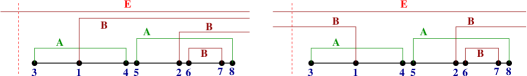
Figure 13: Example of an $A$-irreducible block. $A$- and $B$-contractions are distinguished by green and red lines. Vertices standing close to each other (the pairs $(45)$, $(26)$ and $(78)$) belong to the same $G$. There is one internal $B$-contraction connecting the vertices $6$ and $7$ of the block. Two $B$-contractions are leaving the block, which are connected to the vertices $1$ and $2$, running either to the right (vertices $1$ and $2$ for the left diagram and vertex $2$ for the right diagram) or to the left (vertex $1$ for the right diagram). All the $B$-contractions which cross the block are summarized by the upper line. $E$ is the sum of the Laplace variable $E$ plus the sum of all $x$-variables of the $B$-contractions crossing the block. Therefore, for the left diagram, the resolvent corresponding to the left vertical cut is given by ${1\over E-L_{S}(E)}$, and the diagram corresponds to a contribution for $(G^{B})_{12}^{p_{1}p_{2}}(E)$. In contrast, for the right diagram, we get ${1\over E-x_{1}-L_{S}(E-x_{1})}$ for the resolvent, giving a contribution for $(G^{B})_{12}^{p_{1}p_{2}}(E-x_{1})$. Obviously, by shifting $E\rightarrow E+x_{1}$, the contribution from the right diagram coincides with the one of the left diagram.

Let us label the indices of the vertices of those $B$-contractions, which connect the block to other blocks, by $1,2,\dots n$ (in the sequence from left to right) and call them external indices. Obviously, for $n\geq 1$, we interpret the diagram as a contribution to the effective vertex $(G^{B})^{p_{1}\dots p_{n}}_{1\dots n}(E)$ (if the first vertex is $G$) or to $(R^{B})^{p_{1}\dots p_{n}}_{1\dots n}(E)$ (if the first vertex is $R$). The energy variable $E$ is chosen such that the resolvent standing left to the block is of the form ${1\over E-L_{S}(E)}$, according to the diagrammatic rule that the energy variable of the effective vertex must be identical to the one of the resolvent standing left to the vertex. Thereby we get the same result, independent on whether the $B$-contractions run to blocks to the left or to the right of the considered one, see Fig. 13. Therefore, we determine the diagram by the convention that all $B$-contractions go to the right. In this case, the energy variable $E$ is identical to the one corresponding to all $B$-contractions crossing the block. Subsequently, we have to sum over all possibilities to commute the external indices $1,2,\dots,n$ within the block, see Fig. 14, except when the indices belong to the same vertex $G$ or $R$. To each permutation we associate a corresponding fermionic sign for two reasons. First, the effective vertex $(G^{B})^{p_{1}\dots p_{n}}_{1\dots n}(E)$ should be antisymmetric for fermions under permutation of two indices. Secondly, if the external vertex is used as input for the perturbation series (4.2), it is assumed that the $B$-contractions leave the effective vertex in the sequence $1,2,\dots n$ for the determination of the correct sign when this effective vertex is connected to other effective vertices. Therefore, if the original sequence differs from the one used in the effective vertex, as is the case e.g. in Fig. 14, the corresponding fermionic sign has to be corrected by appropriate rules determining the effective vertex. Furthermore, we attribute to the effective vertex all minus signs which occur when the $A$- and $B$-contractions are separated within the $A$-irreducible blocks from each other and from the external indices (again this is an information which is no longer available when the effective vertex is used in the perturbation series (4.2)). In this way, we get for the diagrams depicted in Figs. 13 and 14 the following result

$$(G^{B})_{12}(E)\, \rightarrow \,(\pm)\,(\pm)\,\gamma^{A}_{34}\,\gamma^{A}_{58}\,\gamma^{B}_{67}\,G_{3}(E)\,\Pi_{3}\,G_{1}(E+x_{3})\,\Pi_{13}$$

$$\cdot\,G_{45}(E+x_{13})\,\Pi_{15}\,G_{26}(E+x_{15})\,\Pi_{1256}\,G_{78}(E+x_{1256})\quad\pm\quad(1\leftrightarrow 2)\quad,$$

where we have omitted for simplicity the obvious notation of the Keldysh indices. The resolvents and energy variables are defined via the short-hand notations

$$\Pi_{1\dots n}\,=\,{1\over E\,+\,x_{1\dots n}-L_{S}^{B}(E\,+\,x_{1\dots n})}\quad,\quad x_{1\dots n}\,=x_{1}\,+\dots+\,x_{n}\quad,$$ (262)

where we used the full effective Liouvillian in the denominator, see below. The two sign factors in (4.2) arise when the two $A$-contractions are separated. As one can see, the rule to translate the effective vertex is quite simple. The indices of the energy variables of all vertices is always identical to the indices of the left preceeding resolvent. The resolvents get the indices of all the left vertices of contractions crossing the vertical cut at the position of the resolvent (the indices of all $B$-contractions crossing the diagram and not belonging to the block are contained in the energy variable $E$).

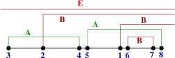
Figure 14: The same diagram as shown in Fig. 13 but the vertices $1$ and $2$ are interchanged. Obviously, since the vertices $1$ and $2$ do not belong to the same vertex $G$, this is a different diagram to the effective vertex $(G^{B})^{p_{1}p_{2}}_{12}(E)$, which has to be counted separately. An additional minus sign has to be considered for fermions since the effective vertex assumes the sequence $12$ for the reservoir lines leaving the vertex.

If no $B$-contractions leave the $A$-irreducible block, we interpret the diagram as a contribution to the effective Liouvillian $L_{S}^{B}(E)$ (if the first vertex is $G$) or to $R_{n=0}^{B}(E)$ (if the first vertex is $R$). An example is shown in Fig. 15, which translates to

$$L^{B}_{S}(E)\,\rightarrow\,{1\over 2}\,\gamma^{A}_{14}\,\gamma^{A}_{23}\,\gamma^{A}_{58}\,\gamma^{B}_{67}\,G_{12}(E)\,\Pi_{12}\,G_{345}(E+x_{12})\,\Pi_{5}\,G_{6}(E+x_{5})\,\Pi_{56}\,G_{78}(E+x_{56})\quad,$$ (263)

where the factor ${1\over 2}$ is a symmetry factor since two vertices are connected by the same contraction within the $A$-irreducible block. As indicated by the definition of the resolvent (262), such diagrams can be resummed on each line connecting the vertices within the $A$-irreducible blocks, leading to the full effective Liouville operator $L_{S}^{B}(E)$ occuring in the denominator of the resolvent. In this way a self-consistent equation is obtained.

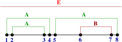
Figure 15: An example of an $A$-irreducible diagram contributing to the effective Liouvillian $L^{B}_{S}(E)$.

Summing up all $A$-irreducible diagrams, we obtain the following perturbation series for the effective Liouvillian and the effective vertices

$$\left\{\begin{array}[]{cl}L_{S}^{B}(E)\\ G^{B}(E)\\ R^{B}(E)\end{array}\right\}\, \rightarrow \,\left\{\begin{array}[]{cl}L_{S}(E)\\ G(E)\\ R(E)\end{array}\right\}\,+\,{1\over S}\,(\pm)^{N_{p}}\,\left(\prod\gamma^{A}\prod\gamma^{B}\right)_{A-irr}\left\{\begin{array}[]{cl}G(E)\\ G(E)\\ R(E)\end{array}\right\}$$

$$\cdot\,{1\over E+X_{1}-L_{S}^{B}(E+X_{1})}\,G(E+X_{1})\,\dots\,{1\over E+X_{r}-L_{S}^{B}(E+X_{r})}\,G(E+X_{r})\quad,$$

where the first term on the r.h.s. represents the original quantities, and the second term contains all $A$-irreducible contributions, indicated by the sub-index $A-irr$ at the product of the contractions. As derived above, we summarize the additional rules

1. All free $B$-contractions are directed to the right. Free $A$-contractions are not allowed.

2. The external indices of the free $B$-contractions are numerated as $1,2,\dots,n$ from left to right.

3. Sum over all permutations of the external indices and assign a minus sign for fermions according to the parity of the permutation. Omit permutations of indices belonging to the same vertex.

4. Associate a fermionic sign which arises when separating all $A$- and $B$-contractions from each other and from the external indices.

Inserting the result (4.2) for the $B$-quantities into the effective perturbation series (4.2) for the physical quantities of interest, we obtain three different terms. The first term on the r.h.s. of (4.2) contains via the two terms on the r.h.s. of (4.2) the original quantities $L_{S}(E)$, $G(E)$ and $R(E)$, together with all $A$-irreducible diagrams. The second term on the r.h.s. of (4.2) contains all $A$-reducible but $B$-irreducible diagrams. In this way one can see that the derivation of a single RG step is nothing else than an obvious classification into different topological sectors, combined with a convenient resummation of $A$-irreducible contributions into effective quantities.

We note that the effective vertices $G^{B}$ and $R^{B}$ are again in normal-ordered form, i.e. in the effective perturbation series (4.2) no $B$-contractions are allowed between field operators belonging to the same $B$-vertex. The reason is that we have incorporated all such terms already into the definition of the effective vertices and the effective Liouvillian by allowing for $B$-contractions on the r.h.s. of Eq. (4.2). In this sense, our RG scheme is quite similiar to the RG scheme developed by Salmhofer salmhofer for quantum field-theoretical problems described by usual Feynman diagrams. However, besides the fact that we have to deal with operator vertices here and have to use the Laplace instead of Fourier transform, an important difference is also that we use the full effective Liouville operator $L_{S}^{B}(E)$ as input for the dynamics of the local quantum system. In this way a self-consistent equation arises for the determination of $L_{S}^{B}(E)$ via (4.2). Transferred to the Salmhofer RG scheme this would mean in a rough sense that self-energy insertions should be resummed on all propagators connecting the vertices, similiar to the RG scheme of Wetterich wetterich (disregarding the fact that both schemes are quite different for many other reasons).

Finally, we mention that one can also set up a non normal-ordered version of the RG procedure. This can be easily achieved by just forbidding the occurence of $B$-contractions on the r.h.s. of (4.2). This means that no $B$-contractions are allowed within the $A$-irreducible blocks which connect the block with itself, see e.g. the $B$-contraction between vertex $6$ and $7$ in Fig. 13. These diagrams are then considered in the non normal ordered effective perturbation series (4.2) by allowing for $B$-contractions connecting field operators from the same $B$-vertex. Concerning usual quantum field-theoretical problems, this would correspond to the RG scheme developed by Polchinski polchinski together with taking the full propagators between the vertices including self-energy insertions. However, as one can see, the normal-ordered version includes more diagrams into the effective quantities and, therefore, the results are expected to be better.

Continuous RG. We can now easily derive the rules for setting up the RG equations (174)-(176) for the continuous RG flow. For a single infinitesimal step $\Lambda\rightarrow\Lambda-d\Lambda$, we use the decomposition (257) with

$$\gamma^{A}\,=\,{d\gamma^{\Lambda}\over d\Lambda}\,d\Lambda\quad,\quad\gamma^{B}\,=\,\gamma^{\Lambda-d\Lambda}\quad.$$ (274)

Comparing (258)-(260) with (4.2) (with $L_{S}\equiv\L_{S}^{\Lambda}$, $G\equiv G^{\Lambda}$ and $R\equiv R^{\Lambda}$), we obtain immediately

$$-\,{d\over d\Lambda}\left\{\begin{array}[]{cl}L_{S}^{\Lambda}(E)\\ G^{\Lambda}(E)\\ R^{\Lambda}(E)\end{array}\right\}\, \rightarrow \,{1\over S}\,(\pm)^{N_{p}}\,\left({d\gamma\over d\Lambda}\prod\gamma^{\Lambda}\right)_{{d\gamma\over d\Lambda}-irr}\,\left\{\begin{array}[]{cl}G^{\Lambda}(E)\\ G^{\Lambda}(E)\\ R^{\Lambda}(E)\end{array}\right\}$$

$$\cdot\,{1\over E+X_{1}-L_{S}^{\Lambda}(E+X_{1})}\,G^{\Lambda}(E+X_{1})\,\dots\,{1\over E+X_{r}-L_{S}^{\Lambda}(E+X_{r})}\,G^{\Lambda}(E+X_{r})\quad,$$

where, for $d\Lambda\rightarrow 0$, we can omit all terms $\sim(d\Lambda)^{k}$ with $k>1$ on the r.h.s., so that only one contraction ${d\gamma\over d\Lambda}$ can occur, and we can replace

$$L_{S}^{B}\equiv L_{S}^{\Lambda-d\Lambda}\rightarrow L_{S}^{\Lambda}\,\,,\,\,G^{B}\equiv G^{\Lambda-d\Lambda}\rightarrow G^{\Lambda}\,\,,\,\,R^{B}\equiv R^{\Lambda-d\Lambda}\rightarrow R^{\Lambda}\,\,,\,\,\gamma^{\Lambda-d\Lambda}\rightarrow\gamma^{\Lambda}$$ (282)

in all other parts of the diagram. Since the total expression has to be irreducible with respect to ${d\gamma\over d\Lambda}$ and only one such contraction is allowed to occur, we get the simple rule that the contraction ${d\gamma\over d\Lambda}$ must contract the first with the last vertex in the diagram, see Figs. 16, 17 and 18 for examples. Diagrammatically this contraction is indicated by an additional slash.

To illustrate the rules, we have shown in Fig. 16 the RG diagrams up to 2-loop order for an arbitrary model with charge fluctuations where the vertex depends only on one index. Omitting the index $\Lambda$ and the trivial Keldysh indices, and using the notation

$$\gamma_{11^{\prime}}\,=\,\delta_{1\bar{1}^{\prime}}\,\gamma_{1}$$ (283)

to exhibit explicitly the $\delta_{1\bar{1}^{\prime}}$-part of each contraction, the RG equations are given by (using again the elegant notation (262))

$$-\,{dL_{S}(E)\over d\Lambda}\, = \,{d\gamma_{1}\over d\Lambda}\,G_{1}(E)\,\Pi_{1}\,G_{\bar{1}}(E+x_{1})$$ (285)

$$+\,{d\gamma_{1}\over d\Lambda}\,\gamma_{2}\,G_{1}(E)\,\Pi_{1}\,G_{2}(E+x_{1})\,\Pi_{12}\,G_{\bar{2}}(E+x_{12})\,\Pi_{1}\,G_{\bar{1}}(E+x_{1})\quad,$$

$$-\,{dG_{1}(E)\over d\Lambda}\, = \,\pm\,{d\gamma_{2}\over d\Lambda}\,G_{2}(E)\,\Pi_{2}\,G_{1}(E+x_{2})\,\Pi_{12}\,G_{\bar{2}}(E+x_{12})\quad.$$ (286)

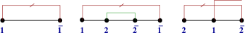
Figure 16: RG diagrams for the Liouvillian and the vertex up to 2-loop order for a model with charge fluctuations. The slash indicates the derivative of the contraction ${d\gamma\over d\Lambda}$.

Note the sign factor in front of (286) due to separating out the contraction between index $2$ and $\bar{2}$ from the external vertex $1$.

Figs. 17 and 18 show the RG diagrams up to 2-loop order for an arbitrary model with spin and orbital fluctuations (44), the Kondo problem (45) being a special example. In this case we get the RG equations

$$-\,{dL_{S}(E)\over d\Lambda}\, = \,{d\gamma_{1}\over d\Lambda}\,\gamma_{2}\,G_{12}(E)\,\Pi_{12}\,G_{\bar{2}\bar{1}}(E+x_{12})$$ (288)

$$+\,{d\gamma_{1}\over d\Lambda}\,\gamma_{2}\,\gamma_{3}\,G_{12}(E)\,\Pi_{12}\,G_{\bar{2}3}(E+x_{12})\,\Pi_{13}\,G_{\bar{3}\bar{1}}(E+x_{13})$$

for the Liouvillian, and

$$-\,{dG_{11^{\prime}}(E)\over d\Lambda}\, = \,\left\{{d\gamma_{2}\over d\Lambda}\,G_{12}(E)\,\Pi_{12}\,G_{\bar{2}1^{\prime}}(E+x_{12})\,\,\pm\,\,(1\leftrightarrow 1^{\prime})\right\}$$ (292)

$$+\,{d\gamma_{2}\over d\Lambda}\,\gamma_{3}\,G_{23}(E)\,\Pi_{23}\,G_{11^{\prime}}(E+x_{23})\,\Pi_{11^{\prime}23}\,G_{\bar{3}\bar{2}}(E+x_{11^{\prime}23})$$

$$\pm\,\left\{{d\gamma_{2}\over d\Lambda}\,\gamma_{3}\,G_{12}(E)\,\Pi_{12}\,G_{1^{\prime}3}(E+x_{12})\,\Pi_{11^{\prime}23}\,G_{\bar{3}\bar{2}}(E+x_{11^{\prime}23})\,\,\pm\,\,(1\leftrightarrow 1^{\prime})\right\}$$

$$+\,\left\{{d\gamma_{2}\over d\Lambda}\,\gamma_{3}\,G_{23}(E)\,\Pi_{23}\,G_{\bar{3}1}(E+x_{23})\,\Pi_{12}\,G_{1^{\prime}\bar{2}}(E+x_{12})\,\,\pm\,\,(1\leftrightarrow 1^{\prime})\right\}$$

for the vertex. The corresponding equations for $R$ follow from replacing the first vertex $G\rightarrow R$. Note the sign factors in front of (292) due to separating out the contraction between index $2$ and $\bar{2}$, and the missing permutation of $1$ and $1^{\prime}$ in (292) since both indices belong to the same vertex. We again note that the energy arguments of the vertices are always such that the indices of the $x$-variable coincide with the indices of the left resolvent. Using these rules, it should be obvious how to write down RG equations in arbitrary order for generic models nearly “without thinking”. However, the problem of course is to solve these RG equations which will be the subject for the rest of the paper.

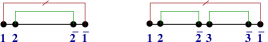
Figure 17: RG diagrams for the Liouvillian up to 2-loop order for a model with spin and/or orbital fluctuations. The slash indicates the derivative of the contraction ${d\gamma\over d\Lambda}$.

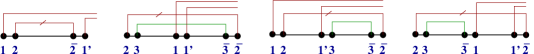
Figure 18: RG diagrams for the vertex up to 2-loop order for a model with spin and/or orbital fluctuations. The slash indicates the derivative of the contraction ${d\gamma\over d\Lambda}$.

4.3 Summary of RG equations and general properties

Summary. We first summarize the RG procedure described in the previous sections. As outlined in Sec. 4.1, we use a 2-stage RG procedure. In the first step we integrate out the symmetric part of the distribution function by a discrete RG step using the decomposition (204)

$$(\gamma^{s})_{11^{\prime}}^{pp^{\prime}}\,=\,\delta_{1\bar{1}^{\prime}}\,p^{\prime}\,\gamma^{s}_{1}\quad,\quad\gamma^{s}_{1}\,=\,{1\over 2}\left\{\begin{array}[]{cl}-\eta\\ 1\end{array}\right\}\,\,\rho_{\nu}(\eta\bar{\omega})\quad,$$ (295)

$$\gamma^{a}_{11^{\prime}}\,=\,\delta_{1\bar{1}^{\prime}}\,\gamma^{a}_{1}\quad,\quad\gamma^{a}_{1}\,=\,\left\{\begin{array}[]{cl}\eta\\ 1\end{array}\right\}\,\,\rho_{\nu}(\eta\bar{\omega})\,\left[f_{\alpha}(\bar{\omega})\pm{1\over 2}\right]\quad,$$ (298)

where we use from now on the conventions

$$\bar{\omega}\,\equiv\,\eta\omega\quad,\quad\bar{\mu}_{\alpha}\,\equiv\,\eta\mu_{\alpha}\quad,\quad x\,\equiv\,\eta(\omega+\mu_{\alpha})\,=\,\bar{\omega}\,+\,\bar{\mu}_{\alpha}\quad,$$ (299)

and

$$\bar{\omega}_{1\dots n}\,=\,\bar{\omega}_{1}+\dots+\bar{\omega}_{n}\quad,\quad\bar{\mu}_{1\dots n}\,=\,\bar{\mu}_{1}+\dots+\bar{\mu}_{n}\quad,\quad x_{1\dots n}\,=\,x_{1}+\dots+x_{n}\quad.$$ (300)

For fermions and $T=0$ we have

$$f_{\alpha}(\bar{\omega})-{1\over 2}\,=\,-\,{1\over 2}\,\mbox{sign}(\bar{\omega})\quad.$$ (301)

The effective Liouvillian $L_{S}^{a}$ and the effective vertices $G^{a}$ and $R^{a}$ are given by (4.2)

$$\left\{\begin{array}[]{cl}L_{S}^{a}(E)\\ G^{a}(E)\\ R^{a}(E)\end{array}\right\}\, \rightarrow \,\left\{\begin{array}[]{cl}L_{S}\\ G\\ R\end{array}\right\}\,+\,{1\over S}\,(\pm)^{N_{p}}\,\left(\prod\gamma^{s}\prod\gamma^{a}\right)_{s-irr}\left\{\begin{array}[]{cl}G\\ G\\ R\end{array}\right\}$$

$$\cdot\,{1\over E+X_{1}-L_{S}^{a}(E+X_{1})}\,G\,\dots\,{1\over E+X_{r}-L_{S}^{a}(E+X_{r})}\,G\quad,$$

where $s-irr$ means irreducibility with respect to the symmetric contractions $\gamma^{s}$. The vertices on the r.h.s. are the initial vertices having no dependence on the energy variable $E$. The energies $X_{i}\equiv x^{(i)}_{1\dots n}$ contain all indices of the left vertex of all contractions crossing the $i$-th resolvent. We also use the convention

$$E_{1\dots n}\,=\,E\,+\,\bar{\mu}_{1\dots n}$$ (312)

such that the energies $X_{i}$ can be written as

$$E\,+\,X_{i}\,\rightarrow\,E\,+\,x_{1\dots n}\,=\,E_{1\dots n}\,+\,\bar{\omega}_{1\dots n}\quad,$$ (313)

separating more clearly the dependence on the integration variables $\bar{\omega}_{i}$ and the physical parameters $E_{1\dots n}$ on which the final solution after integration will depend.

For the next continuous RG procedure we need only the vertices averaged over the Keldysh indices. Therefore, we sum over all Keldysh indices on the r.h.s. of (4.3). Since the Keldysh indices of the initial vertices are all the same, see (77), we obtain only the two possible combinations

$$\bar{G}_{1\dots n}\,=\,\sum_{p}\,G^{pp\dots p}_{1\dots n}\quad,\quad\tilde{G}_{1\dots n}\,=\,\sum_{p}\,p\,G^{pp\dots p}_{1\dots n}$$ (314)

on the r.h.s. of (4.3). Due to the form (295) of the symmetric contraction, $\tilde{G}$ occurs if an odd number of symmetric and left-going contractions are attached to this vertex.

In the second step we replace the remaining antisymmetric contraction $\gamma^{a}$ by the $\Lambda$-dependent contraction (236) with a cutoff defined on the imaginary frequency axis. By convention we write it in the form

$$\gamma_{11^{\prime}}^{\Lambda}\,=\,\delta_{1\bar{1}^{\prime}}\,\gamma_{1}^{\Lambda}\quad$$ (315)

with

$$\gamma_{1}^{\Lambda}\, = \,\left\{\begin{array}[]{cl}\eta\\ -1\end{array}\right\}\,\,\rho_{\nu}(\eta\bar{\omega})\,T\,\sum_{n}\,{1\over\bar{\omega}\,-\,i\omega_{n}^{\alpha}}\,\,\theta_{T_{\alpha}}(\Lambda-|\omega_{n}^{\alpha}|)$$ (318)

$$\begin{array}[b]{c}\vspace{-1.5mm}T\rightarrow 0\\ \longrightarrow\end{array} \left\{\begin{array}[]{cl}\eta\\ -1\end{array}\right\}\,\,\rho_{\nu}(\eta\bar{\omega})\,{1\over 2\pi}\,\int_{-\Lambda}^{\Lambda}d\omega^{\prime}\,{1\over\bar{\omega}\,-\,i\omega^{\prime}}\quad.$$ (323)

The corresponding RG equations are given by (4.2)

$$-\,{d\over d\Lambda}\left\{\begin{array}[]{cl}L_{S}^{\Lambda}(E)\\ \bar{G}^{\Lambda}(E)\\ \bar{R}^{\Lambda}(E)\end{array}\right\}\, \rightarrow \,{1\over S}\,(\pm)^{N_{p}}\,\left({d\gamma\over d\Lambda}\prod\gamma^{\Lambda}\right)_{{d\gamma\over d\Lambda}-irr}\,\left\{\begin{array}[]{cl}\bar{G}^{\Lambda}(E)\\ \bar{G}^{\Lambda}(E)\\ \bar{R}^{\Lambda}(E)\end{array}\right\}$$

$$\cdot\,{1\over E+X_{1}-L_{S}^{\Lambda}(E+X_{1})}\,\bar{G}^{\Lambda}(E+X_{1})\,\dots\,{1\over E+X_{r}-L_{S}^{\Lambda}(E+X_{r})}\,\bar{G}^{\Lambda}(E+X_{r})\quad,$$

where only the vertices (212) averaged over the Keldysh indices occur since the antisymmetric contraction (318) does not depend on the Keldysh indices. The initial condition for these differential equations at $\Lambda=\infty$ is given by

$$L_{S}^{\Lambda=\infty}(E)\, = \,L_{S}^{a}(E)\quad,$$ (331)

$$(\bar{G}^{\Lambda=\infty})_{1\dots n}(E)\, = \,\bar{G}^{a}_{1\dots n}(E)\quad,$$ (332)

$$(\bar{R}^{\Lambda=\infty})_{1\dots n}(E)\, = \,\bar{R}^{a}_{1\dots n}(E)\quad,$$ (333)

where $L_{S}^{a}$, $\bar{G}^{a}$, and $\bar{R}^{a}$ are given by (4.3) from the first discrete step.

Solving the RG equations down to $\Lambda=0$ gives the final result for the physical quantities via (171)

$$L_{S}^{eff}(E)\,=\,L^{\Lambda=0}_{S}(E)\quad,\quad\Sigma_{R}(E)\,=\,R^{\Lambda=0}_{n=0}(E)\quad,$$ (334)

or, alternatively, one can stop the RG at any arbitrary value of $\Lambda$ and use the effective perturbation series (4.1) to calculate the physical quantities

$$\left\{\begin{array}[]{cl}L_{S}^{eff}(E)\\ \Sigma_{R}(E)\end{array}\right\}\, \rightarrow \,\left\{\begin{array}[]{cl}L_{S}^{\Lambda}(E)\\ R^{\Lambda}_{n=0}(E)\end{array}\right\}\,+\,{1\over S}\,(\pm)^{N_{p}}\,\left(\prod\gamma^{\Lambda}\right)_{irr}\left\{\begin{array}[]{cl}\bar{G}^{\Lambda}(E)\\ \bar{R}^{\Lambda}(E)\end{array}\right\}$$

$$\cdot\,{1\over E+X_{1}-L_{S}^{\Lambda}(E+X_{1})}\,\bar{G}^{\Lambda}(E+X_{1})\,\dots\,{1\over E+X_{r}-L_{S}^{\Lambda}(E+X_{r})}\,\bar{G}^{\Lambda}(E+X_{r})\quad.$$

Of course this makes only sense if this perturbation theory is well-defined at the scale $\Lambda$, i.e. if all large terms have already been eliminated by the previous RG flow (which happens when $\Lambda$ reaches some physical low energy scale and the couplings are still small, see the discussion in the following sections).

Symmetry relations. All the symmetry properties from (anti-)symmetry (see (87)), conservation of probability (see (116) and (85)), and those following from the hermiticity of the original Hamiltonian (see (117), (95), (142) and (134)), are also fulfilled for the effective quantities. In summary we have the following relations

$$\hskip 28.45274ptG^{p_{1}\dots p_{i}\dots p_{j}\dots p_{n}}_{1\dots i\dots j\dots n}(E)\,=\,\pm\,G^{p_{1}\dots p_{j}\dots p_{i}\dots p_{n}}_{1\dots j\dots i\dots n}(E)\quad$$ (342)

$$\hskip 28.45274ptR^{p_{1}\dots p_{i}\dots p_{j}\dots p_{n}}_{1\dots i\dots j\dots n}(E)\,=\,\pm\,R^{p_{1}\dots p_{j}\dots p_{i}\dots p_{n}}_{1\dots j\dots i\dots n}(E)\quad,$$ (343)

$$\hskip 34.14322pt\mbox{Tr}_{S}\,L_{S}(E)\,=\,0\quad,\quad\sum_{p_{1}\dots p_{n}}\,\mbox{Tr}_{S}\,G^{p_{1}\dots p_{n}}_{1\dots n}(E)=0\quad,$$ (344)

$$\hskip 73.97733ptL_{S}(E)^{c}\,=\,-L_{S}(-E^{*})\quad,$$ (345)

$$G^{p_{1}\dots p_{n}}_{1\dots n}(E)^{c}\,=\,-\,(\sigma^{-})^{n}\,G^{\bar{p}_{n}\dots\bar{p}_{1}}_{\bar{n}\dots\bar{1}}(-E^{*})\,=\,-\,\sigma^{--\dots-}\,G^{\bar{p}_{1}\dots\bar{p}_{n}}_{\bar{1}\dots\bar{n}}(-E^{*})\quad,$$ (346)

$$R^{p_{1}\dots p_{n}}_{1\dots n}(E)^{c}\,=\,-\,(\sigma^{-})^{n}\,R^{\bar{p}_{n}\dots\bar{p}_{1}}_{\bar{n}\dots\bar{1}}(-E^{*})\,=\,-\,\sigma^{--\dots-}\,R^{\bar{p}_{1}\dots\bar{p}_{n}}_{\bar{1}\dots\bar{n}}(-E^{*})\quad,$$ (347)

where we can either use $L_{S}^{a},G^{a},R^{a}$ or $L_{S}^{\Lambda},\bar{G}^{\Lambda},\bar{R}^{\Lambda}$ for $L_{S},G,R$ (for $\bar{G}$ and $\bar{R}$, the Keldysh indices are of course omitted), a convention we will also use for the following discussions. These identities follow directly from the initial symmetries and the RG equations (4.3) and (4.3), see Appendix D for the proof.

We see that all symmetry properties are preserved under the RG flow. Moreover, they are even invariant within all truncation schemes, since they hold for each term on the r.h.s. of the RG equations separately, provided the complete sum over all indices is taken.

Analytic properties. For a subsequent discussion of the frequency integrations, we first study the analytic properties of the Liouvillian and the vertices in the variables $E$ and $x_{1}\dots x_{n}$. For this, we need the essential ingredient that

$${1\over E-L_{S}(E)}\quad\mbox{is analytic in $E$ in the upper half plane}\quad,$$ (348)

which is equivalent to the property that the effective reduced density matrix, defined by

$$\tilde{\rho}_{S}(E)\,=\,{i\over E-L_{S}(E)}\,\rho_{S}(t_{0})\quad,$$ (349)

has the analytic properties depicted in Fig. 10, i.e. contains no exponentially increasing solutions in time space. To prove this statement generically is difficult since it is not clear whether certain approximations for $L_{S}(E)$ can not lead to poles in the upper half plane. The question is ultimately related to whether the relaxation and dephasing rates generated by the RG flow are positive. So far, we have not seen any mathematical proof to show this property from the structure of the RG equations. Of course we know that, if all terms are taken into account on the r.h.s. of the RG equations, we get the exact solution and at least at the end of the flow, the analytic property (348) must be fulfilled due to physical reasons. Whether it is also fulfilled throughout the RG flow and within certain approximations of the RG equations is not clear and an important question for future research. We will assume in the following that it holds.

From (348) and the analytic structure of the RG equations (4.3) and (4.3), we obtain immediately that

$$L_{S}(E),G(E),R(E)\quad\mbox{are analytic in $E$ in the upper half plane}\quad.$$ (350)

Furthermore, we can also study the analytic properties of the vertices in the frequency variables $x_{1}\dots x_{n}$ with $x_{i}=\eta_{i}(\omega_{i}+\mu_{\alpha_{i}})$ (a better choice than the frequencies $\omega_{i}$ because always this combination occurs in the perturbative series). Writing the vertices as function of the $x$-variables

$$G_{1\dots n}(E)\,\equiv\,G_{\eta_{1}\nu_{1}\dots\eta_{n}\nu_{n}}(E;x_{1}\dots x_{n})\quad,$$ (351)

and assuming that the vertices are analytic in the $x_{i}$-variables initially, we can prove the following analytic property which is preserved under the RG

$$G(E\,+\,x_{1}+\dots+\,x_{m};-x_{1}\dots-x_{m}\,x_{m+1}\dots x_{n})$$

$$\mbox{is analytic if all variables}\quad E,x_{1}\dots x_{n}\quad\mbox{lie in the upper half plane}\quad,$$ (352)

where $1\leq m\leq n$ can take any value. The same holds if any permutation of the indices of the $x$-variables is chosen. It means that the vertices stay analytic in the upper half plane if the sign of some $x_{i}$-variable is changed, provided one replaces $E\rightarrow E+x_{i}$. The property follows from the structure of the RG equations since only the frequency combinations of (352) occur on the r.h.s. Consider e.g. the first term of the RG equation (292), which we write in the representation (351) and integrate out the $\delta$-functions of the contractions by using (315). This gives

$${d\over d\Lambda}\,G_{\eta_{1}\nu_{1},\eta_{1}^{\prime}\nu_{1}^{\prime}}(E;x_{1}x_{1}^{\prime})\, \rightarrow \,{d\gamma_{2}\over d\Lambda}\,\cdot$$

$$\cdot\,G_{\eta_{1}\nu_{1},\eta_{2}\nu_{2}}(E;x_{1}x_{2})\,{1\over E+x_{1}+x_{2}-L_{S}(E+x_{1}+x_{2})}\,G_{-\eta_{2}\nu_{2},\eta_{1}^{\prime}\nu_{1}^{\prime}}(E+x_{1}+x_{2};-x_{2}x_{1}^{\prime})\quad,$$

or for $E\rightarrow E+x_{1}$ and $x_{1}\rightarrow-x_{1}$

$${d\over d\Lambda}\,G_{\eta_{1}\nu_{1},\eta_{1}^{\prime}\nu_{1}^{\prime}}(E+x_{1};-x_{1}x_{1}^{\prime})\, \rightarrow \,{d\gamma_{2}\over d\Lambda}\,\cdot$$

$$\cdot\,G_{\eta_{1}\nu_{1},\eta_{2}\nu_{2}}(E+x_{1};-x_{1}x_{2})\,{1\over E+x_{2}-L_{S}(E+x_{2})}\,G_{-\eta_{2}\nu_{2},\eta_{1}^{\prime}\nu_{1}^{\prime}}(E+x_{2};-x_{2}x_{1}^{\prime})\quad.$$

In all cases we see that the analyticity in $E$, $x_{1}$ and $x_{1}^{\prime}$ is preserved. This holds always because the sign of a $x$-variable can only change due to the $\delta_{12}\sim\delta(x_{1}+x_{2})$ parts of the contractions. Integrating out the right index of each contraction $\gamma_{12}$ leads to the argument $-x_{1}$ for $x_{2}$. However, the vertex $G$ containing the index $2$ stands to the right of the resolvent which the contraction $\gamma_{12}$ crosses, see Fig. 19 for illustration. Therefore, the energy arguments of this vertex are $G(E+x_{1}+\dots;\dots-x_{1}\dots)$. This shows that the structure of the energy arguments is generically of the form shown in (352).

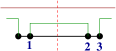
Figure 19: Illustration for the structure of the energy arguments of the vertices. According to the diagrammatic rules, the resolvent and the right vertex have the structure ${1\over E+x_{1}-L_{S}(E+x_{1})}G(E+x_{1};x_{2}x_{3})$. Integrating out the $\delta_{12}\sim\delta(x_{1}+x_{2})$ part of the contraction $\gamma_{12}$, the energy arguments of the vertex get the form $G(E+x_{1};-x_{1}x_{3})$.

These considerations prove that the resolvents and vertices are even analytic with respect to all the internal $x$-variables, e.g. the $x_{2}$-variable in the example above. This will turn out to be quite useful to discuss the frequency integrations over the internal variables. A generic discussion of the frequency integrations is of course not possible since the frequency dependence of the density of states $\rho_{\nu}(\omega)$ and the initial vertices can differ for each model, see e.g. the spin boson model discussed in Sec. 2.2. We discuss here the fermionic case with a flat density of states, i.e. the frequency integrations are performed from minus to plus infinity and we cut off the frequencies of all contractions by the Lorentzian function (47)

$$\rho(\omega)\,=\,{D^{2}\over\omega^{2}+D^{2}}\,=\,{D\over 2i}({1\over\omega-iD}-{1\over\omega+iD})\quad.$$ (355)

Furthermore, the initial vertices are assumed to be analytic functions of the frequencies.

Frequency integrations for the discrete step. We start with the discussion of the frequency integrations for the first discrete RG step where the symmetric part of the contraction is integrated out. Using the analytic properties (348) of the resolvents, the integrations can be performed analytically. When a symmetric contraction crosses over $n$ resolvents in the series (4.3), we get an integral of the type ($z_{i}$ are variables with positive imaginary part)

$$\int d\bar{\omega}\,\rho(\bar{\omega})\,\prod_{i=1}^{n}\,{1\over\bar{\omega}\,+z_{i}-L_{S}^{a}(\bar{\omega}+z_{i})}\,=\,\pi\,D\,\prod_{i=1}^{n}\,{1\over iD\,+z_{i}-L_{S}^{a}(iD+z_{i})}\quad,$$ (356)

i.e. $\bar{\omega}$ is just replaced by $iD$ in all resolvents. This is a very large imaginary part for each denominator and, therefore, this leads to a well-defined perturbation series which can be expanded systematically in the vertices and in $1/D$. Therefore, it is not necessary to take the full Liouvillian $L_{S}^{a}$ in the denominator and solve the equations self-consistently, but one can replace it by the initial value $L_{S}$ and consider the additional diagrams from s-irreducible insertions perturbatively.

Examples of diagrams for the effective Liouvillian are shown in Fig. 20. The first diagram correponds to charge fluctuations and reads for fermions, using the notations (299), (300) and (312)

$$L_{S}^{a}(E)\, \rightarrow \,p^{\prime}\,\gamma_{1}^{s}\,G^{p}_{1}\,{1\over E_{1}\,+\,\bar{\omega}_{1}\,-\,L_{S}}G^{p^{\prime}}_{\bar{1}}\,=\,{1\over 2}\,\bar{G}_{1}\,\int d\bar{\omega}\,\rho(\bar{\omega})\,{1\over\bar{\omega}\,+\,E_{1}\,-\,L_{S}}\,\tilde{G}_{\bar{1}}\quad$$ (357)

$$= \,{1\over 2}\,\bar{G}_{1}\,{\pi D\over iD\,+\,E_{1}\,-\,L_{S}}\,\tilde{G}_{\bar{1}}\,=\,-i\,{\pi\over 2}\,\bar{G}_{1}\,\tilde{G}_{\bar{1}}\,+\,O({1\over D})\quad.$$

Neglecting the contributions $\sim{1\over D}$, we find a result independent of $D$, indicating that such models of charge fluctuations (where the vertex $G_{1}$ has only one index) have a well-defined limit for $D\rightarrow\infty$ if all charge states of the quantum system are taken into account. If the symmetric contraction crosses over more than one resolvent, the result is $\sim{1\over D}$ and can be neglected. Thus, for such models, the determination of the initial condition is very simple.

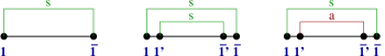
Figure 20: Examples for diagrams of the effective Liouvillian when the symmetric part of the contraction is integrated out in one step. $s$ ($a$) denote the symmetric (antisymmetric) contraction $\gamma^{s}$ ($\gamma^{a}$). Whereas the first diagram is finite for $D\rightarrow\infty$, the other two diagrams contain also terms $\sim D$.

In contrast, the second and third diagrams of Fig. 20 are associated with a model where only spin and/or orbital fluctuations are considered, the Kondo model being a special example. For these models, certain charge excitations have already been integrated out, so that a finite bandwidth $D$ has to be introduced and the limit $D\rightarrow\infty$ is not allowed. In the second diagram the following integral occurs

$$\int d\bar{\omega}\,\rho(\bar{\omega})\,\int d\bar{\omega}^{\prime}\,\rho(\bar{\omega}^{\prime})\,{1\over\bar{\omega}\,+\,\bar{\omega}^{\prime}\,+\,z}\, = \,\int d\bar{\omega}\,\rho(\bar{\omega})\,{\pi D\over\bar{\omega}\,+\,iD\,+\,z}\,=\,{(\pi D)^{2}\over z\,+\,2iD}$$ (358)

$$\,=\,-i\,{\pi^{2}\over 2}\,{D\over 1\,-\,{iz\over 2D}}\,=\,-i\,{\pi^{2}\over 2}\,D\,+\,{\pi^{2}\over 4}\,z\,+\,O({1\over D})\quad,$$

which gives for the diagram the value

$$L_{S}^{a}(E)\, \rightarrow \,{1\over 2}\,\gamma_{1}^{s}\,\gamma_{1^{\prime}}^{s}\,G^{pp}_{11^{\prime}}\,{1\over E_{11^{\prime}}\,+\,\bar{\omega}_{1}\,+\,\bar{\omega}_{1}^{\prime}\,-\,L_{S}}G^{p^{\prime}p^{\prime}}_{\bar{1}^{\prime}\bar{1}}$$ (359)

$$= \,{1\over 8}\,\bar{G}_{11^{\prime}}\,\int d\bar{\omega}\,\rho(\bar{\omega})\,\int d\bar{\omega}^{\prime}\,\rho(\bar{\omega}^{\prime})\,{1\over\bar{\omega}\,+\,\bar{\omega}^{\prime}\,+\,E_{11^{\prime}}\,-\,L_{S}}\,\bar{G}_{\bar{1}^{\prime}\bar{1}}\quad$$

$$= \,-i\,{\pi^{2}\over 16}\,D\,\bar{G}_{11^{\prime}}\,\bar{G}_{\bar{1}^{\prime}\bar{1}}\,+\,{\pi^{2}\over 32}\,\bar{G}_{11^{\prime}}\,(E_{11^{\prime}}\,-\,L_{S})\,\bar{G}_{\bar{1}^{\prime}\bar{1}}\,+\,O({1\over D})\quad.$$

As we can see also terms $\sim D$ are generated which are unphysical since one can prove that the model should contain only logarithmic divergencies $\sim(\ln(D))^{n}$ in higher-order perturbation theory. Such terms occur because the high temperature limit is not well-defined (only temperatures $T<<D$ are allowed since otherwise charge excitations become important which are not considered in the model). As we will see later for the Kondo model in Sec. 5, the terms $\sim D$ will be cancelled by corresponding terms generated in the second continuous RG flow.

Similiarly, also the antisymmetric part of the contraction can occur in the diagrams, see e.g. the third diagram of Fig. 20. It contains more complicated integrals of the form (evaluated here at zero temperature but the same result comes also out at finite $T\ll D$)

$$\int d\bar{\omega}\,\rho(\bar{\omega})\,\left[f_{\alpha}(\bar{\omega})-{1\over 2}\right]\,\int d\bar{\omega}^{\prime}\,\rho(\bar{\omega}^{\prime})\,{1\over\bar{\omega}\,+\,\bar{\omega}^{\prime}\,+\,z}\, = \,\int d\bar{\omega}\,\rho(\bar{\omega})\,\left[f_{\alpha}(\bar{\omega})-{1\over 2}\right]\,{\pi D\over\bar{\omega}\,+\,iD\,+\,z}$$ (360)

$$=\,{\pi D^{3}\over D^{2}\,+\,(z+iD)^{2}}\,\ln(1-{iz\over D})\,=\,{\pi D\over 2}\,{1\over 1\,-\,{iz\over 2D}}\,\,{D\over iz}\,\ln(1-{iz\over D})$$

$$=\,-{\pi\over 2}\,D\,-i\,{\pi\over 2}\,z\,+\,O({1\over D})\quad.$$

This leads to the following value for the third diagram of Fig. 20

$$L_{S}^{a}(E)\, \rightarrow \,p^{\prime}\,\gamma_{1}^{s}\,\gamma_{1^{\prime}}^{a}\,G^{pp}_{11^{\prime}}\,{1\over E_{11^{\prime}}\,+\,\bar{\omega}_{1}\,+\,\bar{\omega}_{1}^{\prime}\,-\,L_{S}}G^{p^{\prime}p^{\prime}}_{\bar{1}^{\prime}\bar{1}}$$ (361)

$$= \,{1\over 2}\,\bar{G}_{11^{\prime}}\,\int d\bar{\omega}\,\rho(\bar{\omega})\,\left[f_{\alpha}(\bar{\omega})-{1\over 2}\right]\,\int d\bar{\omega}^{\prime}\,\rho(\bar{\omega}^{\prime})\,{1\over\bar{\omega}\,+\,\bar{\omega}^{\prime}\,+\,E_{11^{\prime}}\,-\,L_{S}}\,\tilde{G}_{\bar{1}^{\prime}\bar{1}}\quad$$

$$= \,-\,{\pi\over 4}\,D\,\bar{G}_{11^{\prime}}\,\tilde{G}_{\bar{1}^{\prime}\bar{1}}\,-\,i\,{\pi\over 4}\,\bar{G}_{11^{\prime}}\,(E_{11^{\prime}}\,-\,L_{S})\,\tilde{G}_{\bar{1}^{\prime}\bar{1}}\,+\,O({1\over D})\quad.$$

A similiar structure as compared to the other diagram (359) occurs. This illustrates that the symmetric part can be integrated out using perturbation theory in the coupling vertices. No logarithmic divergencies $\sim\ln(D/|E_{1\dots n}-L_{S}|)$ can occur in any order since the upper limit of all integrals and the cutoff provided in the denominators of all resolvents is given by the bandwidth $D$.

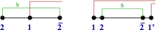
Figure 21: Examples for diagrams of the effective vertices when the symmetric part of the contraction is integrated out in one step. $s$ ($a$) denote the symmetric (antisymmetric) contraction $\gamma^{s}$ ($\gamma^{a}$). Whereas the left diagram is negligible for $D\rightarrow\infty$, the right diagram is finite.

Examples for diagrams for the determination of the effective vertices are shown in Fig. 21. The first diagram corresponds to charge fluctuations. It is of order $O({1\over D})$ and can be neglected

$$\bar{G}_{1}(E)\, \rightarrow \,p_{2}^{\prime}\,\gamma^{s}_{2}\,G^{p_{2}}_{2}\,{1\over E_{2}\,+\,\bar{\omega}_{2}\,-\,L_{S}}\,G^{p}_{1}\,{1\over E_{12}\,+\,\bar{\omega}_{1}\,+\,\bar{\omega}_{2}\,-\,L_{S}}\,G^{p_{2}^{\prime}}_{\bar{2}}$$

$$= \,{1\over 2}\,\int d\bar{\omega}_{2}\,\rho(\bar{\omega}_{2})\,\bar{G}_{2}\,{1\over\bar{\omega}_{2}\,+\,E_{2}\,-\,L_{S}}\,\bar{G}_{1}\,{1\over\bar{\omega}_{2}\,+\,E_{12}\,+\,\bar{\omega}_{1}\,-\,L_{S}}\,\tilde{G}_{\bar{2}}\,\sim\,O({1\over D})\quad.$$

The second diagram corresponds to spin/orbital fluctuations and is finite in the limit $D\rightarrow\infty$

$$\bar{G}_{11^{\prime}}(E)\, \rightarrow \,p^{\prime}\,\gamma^{s}_{2}\,G^{pp}_{12}\,{1\over E_{12}\,+\,\bar{\omega}_{1}\,+\,\bar{\omega}_{2}\,-\,L_{S}}\,G^{p^{\prime}p^{\prime}}_{\bar{2}1^{\prime}}\,-\,(1\leftrightarrow 1^{\prime})$$ (363)

$$= \,{1\over 2}\,\bar{G}_{12}\,\int d\bar{\omega}_{2}\,\rho(\bar{\omega}_{2})\,{1\over\bar{\omega}_{2}\,+\,E_{12}\,+\,\bar{\omega}_{1}\,-\,L_{S}}\,\tilde{G}_{\bar{2}1^{\prime}}\,-\,(1\leftrightarrow 1^{\prime})$$

$$= \,{1\over 2}\,\bar{G}_{12}\,{\pi D\over iD\,+\,E_{12}\,+\,\bar{\omega}_{1}\,-\,L_{S}}\,\tilde{G}_{\bar{2}1^{\prime}}\,-\,(1\leftrightarrow 1^{\prime})$$

$$= \,-i\,{\pi\over 2}\,\left(\bar{G}_{12}\,\tilde{G}_{\bar{2}1^{\prime}}\,-\,\bar{G}_{1^{\prime}2}\,\tilde{G}_{\bar{2}1}\right)\,+\,O({1\over D})\quad.$$

In conclusion, we see that for initial vertices with one index (charge fluctuations), the effective Liouvillian is finite for $D\rightarrow\infty$ and the effective vertices are identical to the initial ones. For initial vertices with two indices (spin and/or orbital fluctuations), the effective Liouvillian contains also terms $\sim D$ and the effective vertices get a finite correction to the initial ones. Initial vertices with three indices correspond to quite artificial models, in that case also terms $\sim D^{2}$ can occur for the effective Liouvillian and terms $\sim D$ for the effective vertices.

Furthermore, we note that the effective Liouvillian can contain terms which are linear in the energy $E$, see (359) and (361). This does not lead to a problem for arbitrarily large frequencies because the effective Liouvillian occurs always in the denominator of all resolvents of the effective perturbation series or the r.h.s. of the RG equations. In contrast, the effective vertices are independent of frequency, see (363), which is important for a well-defined large frequency behaviour of all expressions.

Frequency integrations for the continuous RG equations. We now turn to the frequency integrations of the RG equations (4.3) of the continuous RG flow. From the form of the contraction (318), we see that by closing the integrations over $\bar{\omega}$ in the upper half of the complex plane, only the pole from the Matsubara frequency $\omega_{n}^{\alpha}$ and the pole of the Lorentzian cutoff function (355) at $iD$ contributes (we again replace $\rho_{\nu}(\omega)$ by (355) in all contractions). All other resolvents and vertices are analytic in the upper half plane, according to (348) and (352). Most importantly, the contraction ${d\gamma\over d\Lambda}$, which is differentiated with respect to $\Lambda$, crosses over all resolvents (to make the expression ${d\gamma\over d\Lambda}$-irreducible), i.e. the frequency variable of that contraction occurs in all resolvents! Moreover, due to the derivative, we get for this contraction from (318)

$${d\gamma_{1}^{\Lambda}\over d\Lambda}\, = \,\left\{\begin{array}[]{cl}\eta\\ -1\end{array}\right\}\,\,\rho(\bar{\omega})\,T\,\sum_{n}\,{1\over\bar{\omega}\,-\,i\omega_{n}^{\alpha}}\,\,\delta_{T_{\alpha}}(\Lambda-|\omega_{n}^{\alpha}|)$$ (366)

$$= \,\left\{\begin{array}[]{cl}\eta\\ -1\end{array}\right\}\,\,\rho(\bar{\omega})\,{1\over 2\pi}\,\,\left({1\over\bar{\omega}\,-\,i\Lambda_{T_{\alpha}}}\,+\,{1\over\bar{\omega}\,+\,i\Lambda_{T_{\alpha}}}\right)\quad,$$ (369)

where $\delta_{T}(\omega)$ is a delta function smeared by temperature, defined as the derivative of $\theta_{T}(\omega)$, given by (217), i.e.

$$\delta_{T}(\omega)\,=\,{d\over d\omega}\,\theta_{T}(\omega)\,=\,\left\{\begin{array}[]{cl}0&\quad\mbox{for }|\omega|\,>\,\pi T\\ {1\over 2\pi T}&\quad\mbox{for }|\omega|\,<\,\pi T\end{array}\right.\quad.$$ (370)

As a consequence, only the two Matsubara frequencies $\pm\Lambda_{T_{\alpha}}$ lying closest to $\pm\Lambda$ contribute to the sum in Eq. (366), and we obtain exactly Eq. (369). Therefore, we get the important result that, by closing the frequency integration of ${d\gamma\over d\Lambda}$ in the upper half plane, the contribution from the Matsubara poles gives rise to the replacement

$$\bar{\omega}\,\rightarrow\,i\Lambda_{T_{\alpha}}\quad\mbox{in {\it all} resolvents of the r.h.s. of the RG equation (\ref{rg_equations}).}$$ (371)

Therefore, a large positive imaginary part occurs in all resolvents so that the perturbative series on the r.h.s. of the RG equations is well-defined provided that the coupling constants remain small. In contrast, the Matsubara poles from all the other contractions occur only in those resolvents where the contractions cross over.

The pole at $iD$ from the density of states is only important if one wants to study the precise behaviour of the RG flow when $\Lambda$ crosses the bandwidth $D$. However, nothing really interesting is happening in that regime, except for the fact that $D$ sets the scale where the divergencies of the original perturbation theory are cut off at high energies, i.e. at $\Lambda\sim D$ the RG flow starts to renormalize the effective parameters significantly. To see this analytically, we perform the integration over the frequency variable $\bar{\omega}$ of the ${d\gamma\over d\Lambda}$ contraction analytically. Using (369) with (355) we obtain by closing in the upper half of the complex plane

$$\int d\bar{\omega}\,\rho(\bar{\omega})\,{1\over 2\pi}\,({1\over\bar{\omega}\,-\,i\Lambda_{T_{\alpha}}}\,+\,{1\over\bar{\omega}\,+\,i\Lambda_{T_{\alpha}}})\,\left\{\dots\right\}_{\bar{\omega}}\,=$$ (372)

$$=\,-i\,{D^{2}\over\Lambda_{T_{\alpha}}^{2}-D^{2}}\,\left[\left\{\dots\right\}_{\bar{\omega}=i\Lambda_{T_{\alpha}}}\,-\,\left\{\dots\right\}_{\bar{\omega}=iD}\right]\quad,$$

where $\{\dots\}_{\bar{\omega}}$ stands for the rest of the diagram. We see that for $\Lambda\gg D$, there is small prefactor $\sim({D\over\Lambda})^{2}\ll 1$ in front of the r.h.s. of the RG equations leading to a negligible renormalization. In contrast, for $\Lambda\ll D$, the prefactor is $i$ and the renormalization becomes important. In this regime, only the term $\{\dots\}_{\bar{\omega}=i\Lambda_{T_{\alpha}}}$ has to be considered on the r.h.s. of (372) and the r.h.s. of the RG equation becomes independent of $D$.

In summary, the RG flow will roughly start at $\Lambda\sim D$ but the precise value where it starts is not so important since the cutoff $D$ occurs logarithmically in the divergencies of perturbation theory. Therefore, it is a good approximation to evaluate the r.h.s. of the RG equations for $\Lambda\ll D$, and use $D$ just as the starting value of the flow parameter $\Lambda$, where the initial values of the Liouvillian and the vertices are taken from the first discrete RG step. Moreover, as we will see in more detail in connection with the application to the Kondo problem in Sec. 5, the precise ratio of the initial value of $\Lambda$ and the bandwidth $D$ should be chosen in such a way that the terms linear in $D$ of the initial Liouvillian cancel out (as it should be since such terms do not exist in the original perturbation theory).

As a consequence we consider from now on only the regime $\Lambda\ll D$ and omit the cutoff function $\rho(\bar{\omega})$ in all contractions. We then close the integrations over all variables $\bar{\omega}_{i}$ in the upper half plane and replace them by the pole of the Matsubara frequencies in all resolvents and vertices of the diagram. As a result we find the same form of the RG equations but with the replacements

$$\gamma_{1}^{\Lambda}\,,\,{d\gamma_{1}^{\Lambda}\over d\Lambda}\rightarrow\,i\,\left\{\begin{array}[]{cl}\eta\\ -1\end{array}\right\}$$ (373)

for all contractions, together with

$$\bar{\omega}\,\rightarrow\,i\omega_{n}^{\alpha}\quad,\quad\int d\bar{\omega}\,\rightarrow\,2\pi T_{\alpha}\sum_{0<\omega_{n}^{\alpha}}\theta_{T_{\alpha}}(\Lambda-\omega_{n}^{\alpha})$$ (374)

for the frequency variables of all contractions $\gamma^{\Lambda}_{1}$, and

$$\bar{\omega}\,\rightarrow\,i\Lambda_{T_{\alpha}}$$ (375)

for the frequency variable of the contraction ${d\gamma^{\Lambda}_{1}\over d\Lambda}$. Note that only positive Matsubara frequencies are allowed in the sum.

RG on Matsubara axis. When the integrations over all real frequencies are performed, the energy variables $E+X_{i}$ of the RG equations (4.3) get the form

$$E\,+\,X_{i}\,\rightarrow\,E\,+\,\bar{\mu}_{1\dots n}\,+\,i\Lambda_{T_{\alpha_{1}}}\,+\,i\omega_{2\dots n}\quad,$$ (376)

where index $1$ is assumed to be the variable of ${d\gamma^{\Lambda}_{1}\over d\Lambda}$, and

$$\omega_{1\dots k}\,=\,\omega_{n_{1}}^{\alpha_{1}}\,+\dots+\,\omega_{n_{k}}^{\alpha_{k}}$$ (377)

is the sum over the Matsubara frequencies in analogy to the notation (300). We see that the value for the energies $E$ appearing in the Liouvillian $L_{S}(E)$ and the vertices $\bar{G}_{1\dots n}(E)$ are complex numbers with the imaginary part being some positive Matsubara frequency. Thus, we can reformulate the whole RG equations for frequencies on the Matsubara axis by replacing all variables $\bar{\omega}$ by Matsubara frequencies and using for $E$ a real part plus some Matsubara frequency. With this, only the following quantities occur in the RG equations

$$L_{S}(E;\omega)\, = \,L_{S}(E+i\omega)\quad,$$

$$\bar{G}_{1\dots n}(E,\omega,\omega_{1}\dots\omega_{n}) \equiv \bar{G}_{\eta_{1}\nu_{1}\dots\eta_{n}\nu_{n}}(E,\omega,\omega_{1}\dots\omega_{n})\,=\,\bar{G}_{1\dots n}(E+i\omega)|_{\bar{\omega}_{i}\rightarrow i\omega_{i}}\quad,$$ (378)

where $\omega,\omega_{1}\dots\omega_{n}$ are positive Matsubara frequencies and $E$ is real. By convention, if the frequencies are written explicitly in the arguments, the index $1\equiv\eta\nu$ does no longer contain the frequency. The RG equations in Matsubara space for $L_{S}(E,\omega)$ and $\bar{G}_{\dots}(E,\omega,\dots)$ are obtained from the original RG equations by the replacements

$$\gamma_{1}^{\Lambda}\,,\,{d\gamma_{1}^{\Lambda}\over d\Lambda} \rightarrow \,i\,\left\{\begin{array}[]{cl}\eta\\ -1\end{array}\right\}\quad,$$ (381)

$$\Pi_{1\dots n}\, \rightarrow \,\Pi(E_{1\dots n},\omega+\omega_{1\dots n})\quad,$$ (382)

$$\bar{G}_{1\dots n}(E+x_{1^{\prime}\dots n^{\prime}})\, \rightarrow \,\bar{G}_{1\dots n}(E_{1^{\prime}\dots n^{\prime}},\omega+\omega_{1^{\prime}\dots n^{\prime}},\omega_{1}\dots\omega_{n})\quad,$$ (383)

$$\omega_{1}\, \rightarrow \,\Lambda_{T_{\alpha_{1}}}\quad\mbox{for }{d\gamma_{1}\over d\Lambda}\quad,$$ (384)

$$\int d\omega\, \rightarrow \,2\pi{T_{\alpha}}\,\sum_{0<\omega^{\alpha}_{n}}\theta_{T_{\alpha}}(\Lambda-\omega_{n}^{\alpha})\,\quad\mbox{for }\gamma_{1}\quad,$$ (385)

where all frequencies correspond to Matsubara frequencies $\omega_{i}\equiv\omega_{n_{i}}^{\alpha_{i}}$, and we have used the convention $E_{1\dots n}=E+\bar{\mu}_{1\dots n}$ together with the definition

$$\Pi(E,\omega)\,=\,{1\over E\,+\,i\omega\,-\,L_{S}(E,\omega)}\quad.$$ (386)

Furthermore, the explicit frequency arguments of the resolvent and the vertices in Matsubara space can be avoided by the compact notation

$$\bar{G}^{M}_{1\dots n}(E_{1^{\prime}\dots n^{\prime}})\, \equiv \,\bar{G}_{1\dots n}(E_{1^{\prime}\dots n^{\prime}},\omega+\omega_{1^{\prime}\dots n^{\prime}},\omega_{1}\dots\omega_{n})\quad,$$ (387)

$$\pi^{M}_{1\dots n}\, \equiv \,\Pi(E_{1\dots n},\omega+\omega_{1\dots n})\quad,$$ (388)

which is especially useful for writting down higher-order terms of the RG equations. In this notation the Matsubara RG equations have nearly the same form as the original RG equations besides the replacements (381) for the contractions. However, one should note that the external frequency variable $\omega$ is hidden in this notation and one has to specify explicitly which variable is set on the parameter $\Lambda_{T_{\alpha}}$.

As an example consider the RG equations (285)-(286) for a model with charge fluctuations. Using the above rules in the representation (378), we get immediately

$$-\,{dL_{S}(E,\omega)\over d\Lambda}\, = \,-i\,\bar{G}_{1}(E,\omega,\Lambda_{T_{\alpha_{1}}})\,\Pi(E_{1},\omega+\Lambda_{T_{\alpha_{1}}})\,\bar{G}_{\bar{1}}(E_{1},\omega+\Lambda_{T_{\alpha_{1}}},-\Lambda_{T_{\alpha_{1}}})$$ (390)

$$-\,\bar{G}_{1}(E,\omega,\Lambda_{T_{\alpha_{1}}})\,\Pi(E_{1},\omega+\Lambda_{T_{\alpha_{1}}})\,\bar{G}_{2}(E_{1},\omega+\Lambda_{T_{\alpha_{1}}},\omega_{2})\,\Pi(E_{12},\omega+\Lambda_{T_{\alpha_{1}}}+\omega_{2})\,\cdot$$

$$\cdot\,\bar{G}_{\bar{2}}(E_{12},\omega+\Lambda_{T_{\alpha_{1}}}+\omega_{2},-\omega_{2})\,\Pi(E_{1},\omega+\Lambda_{T_{\alpha_{1}}})\,\bar{G}_{\bar{1}}(E_{1},\omega+\Lambda_{T_{\alpha_{1}}},-\Lambda_{T_{\alpha_{1}}})\quad,$$

$$-\,{d\bar{G}_{1}(E,\omega,\omega_{1})\over d\Lambda}\, = \,i\,\bar{G}_{2}(E,\omega,\Lambda_{T_{\alpha_{2}}})\,\Pi(E_{2},\omega+\Lambda_{T_{\alpha_{2}}})\,\bar{G}_{1}(E_{2},\omega+\Lambda_{T_{\alpha_{2}}},\omega_{1})\,\cdot$$

$$\cdot\,\Pi(E_{12},\omega+\omega_{1}+\Lambda_{T_{\alpha_{2}}})\,\bar{G}_{\bar{2}}(E_{12},\omega+\omega_{1}+\Lambda_{T_{\alpha_{2}}},-\Lambda_{T_{\alpha_{2}}})\quad.$$ (391)

Using the compact notation (387) and (388), the RG equations (288)-(292) for a model with arbitrary spin and/or orbital fluctuations read for fermions

$$-\,{dL_{S}(E,\omega)\over d\Lambda}\, = \,-\,\bar{G}^{M}_{12}(E)\,\pi^{M}_{12}\,\bar{G}^{M}_{\bar{2}\bar{1}}(E_{12})\,|_{\omega_{1}=\Lambda_{T_{\alpha_{1}}}}$$ (393)

$$+\,i\,\bar{G}^{M}_{12}(E)\,\pi^{M}_{12}\,\bar{G}^{M}_{\bar{2}3}(E_{12})\,\pi^{M}_{13}\,\bar{G}^{M}_{\bar{3}\bar{1}}(E_{13})\,|_{\omega_{1}=\Lambda_{T_{\alpha_{1}}}}\quad,$$

$$-\,{d\bar{G}_{11^{\prime}}(E,\omega,\omega_{1},\omega_{1}^{\prime})\over d\Lambda}\, = \,-i\,\left\{\bar{G}^{M}_{12}(E)\,\pi^{M}_{12}\,\bar{G}^{M}_{\bar{2}1^{\prime}}(E_{12})\,\,-\,\,(1\leftrightarrow 1^{\prime})\right\}\,|_{\omega_{2}=\Lambda_{T_{\alpha_{2}}}}$$ (397)

$$-\,\bar{G}^{M}_{23}(E)\,\pi^{M}_{23}\,\bar{G}^{M}_{11^{\prime}}(E_{23})\,\pi^{M}_{11^{\prime}23}\,\bar{G}^{M}_{\bar{3}\bar{2}}(E_{11^{\prime}23})\,|_{\omega_{2}=\Lambda_{T_{\alpha_{2}}}}$$

$$+\,\left\{\,\bar{G}^{M}_{12}(E)\,\pi^{M}_{12}\,\bar{G}^{M}_{1^{\prime}3}(E_{12})\,\pi^{M}_{11^{\prime}23}\,\bar{G}^{M}_{\bar{3}\bar{2}}(E_{11^{\prime}23})\,\,-\,\,(1\leftrightarrow 1^{\prime})\right\}\,|_{\omega_{2}=\Lambda_{T_{\alpha_{2}}}}$$

$$-\,\left\{\,\bar{G}^{M}_{23}(E)\,\pi^{M}_{23}\,\bar{G}^{M}_{\bar{3}1}(E_{23})\,\pi^{M}_{12}\,\bar{G}^{M}_{1^{\prime}\bar{2}}(E_{12})\,\,-\,\,(1\leftrightarrow 1^{\prime})\right\}\,|_{\omega_{2}=\Lambda_{T_{\alpha_{2}}}}\quad.$$

For the final physical quantities, we need according to (334)

$$L_{S}^{eff}(E)\,=\,L^{\Lambda=0}_{S}(E,\omega=0)\quad,\quad\Sigma_{R}(E)\,=\,R^{\Lambda=0}_{n=0}(E,\omega=0)\quad,$$ (398)

i.e. we can fix $E$ in the RG equations and see that only $E$ shifted by the discrete set of values $\bar{\mu}_{1\dots n}$ occurs for the first frequency variable. This means that the RG equations are local in Laplace space up to a shift by multiples of the chemical potentials of the reservoirs. This simplifies the calculation of the time evolution considerably. E.g. if only two reservoirs with $\mu_{L}=-\mu_{R}={V\over 2}$ are present, we get $n{V\over 2}$ with $n=0,\pm 1,\pm 2,\dots$ for $\bar{\mu}_{1\dots n}$, i.e. only the fixed Laplace variable shifted by multiples of half the bias voltage can occur for the first frequency variable of the Liouvillian and the vertices.

In summary, we find that the RG can be formulated on the Matsubara axis but in contrast to equilibrium Matsubara formalism, there is a whole set of Matsubara axis shifted by the real quantities

$$E\,+\,n_{1}\mu_{1}\,+\dots+\,n_{Z}\,\mu_{Z}\quad,\quad n_{i}=0,\pm 1,\pm 2,\dots$$ (399)

where $Z$ is the number of reservoirs, $\mu_{k}$ is the chemical potential of reservoir $k$, and $E$ is the real part of the Laplace variable. This is the price one has to pay compared to equilibrium to calculate the time evolution and the effect from different chemical potentials. If different temperatures of the reservoirs occur (leading to nonequilibrium heat currents), the Matsubara frequency axis has to be defined for each reservoir individually.

Finally, we note that within our formalism no analytic continuation to real frequencies is necessary to calculate the time evolution of the average over an arbitrary observable (the same holds for correlation functions not shown in this paper). This is an advantage compared to the usual linear response formalism kubo or to recently developed nonequilibrium formalism with complex chemical potentials QMC , where an analytic continuation is necessary. In this way we can avoid the numerical problems associated with analytic continuations.

Cutoff parameters for the RG flow. Using the form (376) together with the representation (378), and replacing the effective Liouvillian by its eigenvalue via (184), we find the following structure of each resolvent of the RG equation

$${1\over E\,+\,\bar{\mu}_{1\dots n}\,-\,h_{k}^{\Lambda}\,+\,i\Lambda_{T_{\alpha_{1}}}\,+\,i\omega\,+\,i\omega_{2\dots n}\,+\,i\Gamma_{k}^{\Lambda}}\quad,$$ (400)

where $\omega$ is the Matsubara frequency associated with the energy variable $E$. The energy arguments of the real and imaginary parts $h_{k}^{\Lambda},\Gamma_{k}^{\Lambda}$ of the eigenvalues of the effective Liouvillian at scale $\Lambda$ are not indicated (which is the same energy as occuring in the rest of the resolvent). As already mentioned in Sec. 4.1, this form of the resolvents is very useful for stable numerical calculations since all imaginary parts in the denominator are positive. Furthermore, it shows generically what the various cutoff parameters of the RG flow are. If the flow parameter $\Lambda$ falls roughly below the value ($E$ is assumed to be real here)

$$\Lambda\,<\,\mbox{max}\left\{T_{\alpha}\,,\,|E+\bar{\mu}_{1\dots n}-h_{k}^{\Lambda}|\,,\,\omega\,,\,\omega_{2}\,,\,\dots\,,\,\omega_{n}\,,\,\Gamma_{k}^{\Lambda}\right\}\quad,$$ (401)

the resolvent (400) becomes approximately a constant, cutting off logarithmic divergencies for low energies. In this way the temperatures $T_{\alpha}$ of the reservoirs, the Laplace variable $E$, the chemical potentials $\mu_{\alpha}$ of the reservoirs, the oscillation frequencies $h_{k}$, the Matsubara frequencies $\omega_{n}^{\alpha}$, and the relaxation and dephasing rates $\Gamma_{k}$ serve as cutoff parameters. The cutoff occurs in a natural way and in an intuitively expected form in the RG equations. However, in contrast to temperature and the imaginary parts of the resolvent, one should note that only the combination $E+\bar{\mu}_{1\dots n}-h_{k}^{\Lambda}$ is the cutoff parameter in the real part of the denominator. Therefore, there are interesting points when this combination is zero

$$E\,+\,\bar{\mu}_{1\dots n}\,-\,h_{k}\,=\,0\quad,$$ (402)

where enhanced renormalizations are expected. These points correspond physically to resonances. E.g. for the Kondo model they lead to an additional logarithmic enhancement of the differential conductance when the external magnetic field is identical to the bias voltage, see e.g. Ref. reininghaus_hs_preprint for a detailed study of this problem using RTRG-FS or Refs. rosch_paaske_kroha_woelfle_PRL03 ; paaske_rosch_woelfle_PRB04 ; glazman_pustilnik_05 where other methods have been used). A nice feature of the RTRG-FS procedure presented here is that, without specifying the model at all, we can generically predict that logarithmic enhancements are expected when the condition (402) is fulfilled.

In contrast, temperature is always a cutoff scale because when $\Lambda$ falls below $T_{\alpha}$, the last Matsubara frequency has been integrated out and the RG flow stops. Compared to equilibrium, this means for nonequilibrium problems that the voltage (inducing nonequilibrium stationary states) and the Laplace variable $E$ (determining the time evolution of an initially out of equilibrium state) induce different cutoff behaviours of the RG equations than temperature. All resolvents on the r.h.s. of the RG equations have a different structure concerning the combination of energy variables $E+\bar{\mu}_{1\dots n}-h_{k}$. In equilibrium, only the eigenvalues $h_{k}$ can occur but they can not be cancelled by other energy variables. This opens up many new interesting physical phenomena for nonequilibrium systems to be studied in the future.

As temperature, also the Matsubara frequencies and the relaxation and dephasing rates will cut off the RG flow and can not be cancelled in the denominator since they are all positive. Most importantly, as has already been discussed in all detail in Sec. 4.1, the zero eigenvalue of the effective Liouvillian can not occur in the resolvents. This means that we have found a generic proof that relaxation and dephasing rates will always cut off the RG flow, irrespective of the truncation scheme used and of the specific model under consideration.

4.4 Weak coupling limit

Definition of weak coupling. We start with the definition of weak coupling by defining the dimensionless “coupling constant” $J_{\Lambda}$ at scale $\Lambda$

$$J_{\Lambda}\,\equiv\,\Lambda^{{n\over 2}-1}\,G^{\Lambda}_{1\dots n}\quad,$$ (403)

where, from now on, we use the definition (20) for the field operators such that $a_{\nu}(\omega)$ has dimension ${1\over\sqrt{E}}$. The connection between the RG equations for $J_{\Lambda}$ and $G^{\Lambda}$ is

$${dJ_{\Lambda}\over dl}\,=\,(1-{n\over 2})\,J_{\Lambda}\,-\,\Lambda^{n\over 2}\,{dG^{\Lambda}\over d\Lambda}\quad,\quad l\,=\,\ln({D\over\Lambda})\quad,$$ (404)

where $l$ is a dimensionless flow parameter running from $l=0$ at $\Lambda=D$ to $l=\infty$ at $\Lambda=0$. Here, the first term describes the trivial renormalization of $J_{\Lambda}$ by the rescaling factor in (403), whereas the second one stems from the renormalization of $G^{\Lambda}$. If we rescale all energies in the RG equation for $G^{\Lambda}$ by $\Lambda$, the second term on the r.h.s. of (404) is a power series in $J_{\Lambda}$ starting at $J_{\Lambda}^{2}$ for $n>1$ and at $J^{3}_{\Lambda}$ for $n=1$, see the RG diagrams of Fig. 16 for $n=1$ and Fig. 18 for $n=2$. For a term $\sim J^{k}_{\Lambda}$, there are $k-1$ resolvents in between, so we estimate the term in this order as

$$\Lambda^{n\over 2}\,{dG^{\Lambda}\over d\Lambda}\,\rightarrow\,J_{\Lambda}^{k}\,\left\{\begin{array}[]{cl}({\Lambda\over\Delta})^{k-1}&\mbox{for }\Lambda\ll\Delta\\ O(1)&\mbox{for }\Lambda\gg\Delta\end{array}\right.\quad,$$ (405)

where $\Delta$ stands symbolically for all the physical scales occuring in the denominator of the resolvents according to (400), i.e.

$$\Delta\,\sim\,T\,,\,E+\bar{\mu}_{1\dots n}-h\,,\,\Gamma\quad,$$ (406)

except for the frequencies which are rescaled by $\Lambda$ and will give something of order $O(1)$ in the denominator of the resolvent (note that all frequency integrations are cut off by $\Lambda$, they all give a positive contribution to the imaginary part of the denominator, and $i\Lambda$ occurs in all resolvents).

Weak coupling means that the expansion (405) of the expression $\Lambda^{n\over 2}\,{dG^{\Lambda}\over d\Lambda}$ in a power series in $J_{\Lambda}$ is under control for all values of the flow parameter, which is the case if the condition

$$J_{\Lambda}\ll 1\quad\mbox{or}\quad\Lambda\ll\Delta$$ (407)

is always fulfilled. Only in this case truncation schemes on the r.h.s. of the RG equations are justified, leading to a well-defined renormalized perturbation series in $J$. We discuss this condition now for the possible values of $n$ in (404), where $n$ is the number of field operators of the considered vertex $G^{\Lambda}_{1\dots n}$.

For $n>2$, the weak-coupling condition is certainly not a problem since already the first term of (404) leads to a reduction of $J$. Therefore these terms are called irrelevant in the renormalization group sense.

For $n=2$ (e.g. spin and/or orbital fluctuations) we have $J_{\Lambda}=G^{\Lambda}$ and the first term on the r.h.s. of (404) is zero. By convention, this is called the marginal case. The weak-coupling condition (407) will be fulfilled if the renormalized coupling $J_{\Lambda}$ stays small until $\Lambda$ reaches the cutoff scale $\Delta$. Under this condition, $J_{\Lambda}$ will also stay small for $\Lambda<\Delta$, since an additional factor $\sim({\Lambda\over\Delta})^{k-1}$ appears in this regime, see (405). Since the smallest cutoff scale is the minimum of all relaxation and dephasing rates of the problem, we obtain the condition (178)

$$\min_{i}\,\left\{\Gamma_{i}\right\}\,\gg\,T_{K}\quad\Rightarrow\quad\mbox{weak coupling}\quad,$$ (408)

where $T_{K}$ is defined as the energy scale where the coupling $J_{\Lambda=T_{K}}\sim O(1)$ if all physical cutoff scales $\Delta$ are disregarded.

For $n=1$ (e.g. charge fluctuations) the first term on the r.h.s. of (404) leads to an increase of $J$, therefore this situation is called the relevant case. Due to the relations (39) and (40), we expect $G^{\Lambda}\sim\sqrt{\Gamma^{\Lambda}}$ and we obtain

$$J_{\Lambda}\,=\,{1\over\sqrt{\Lambda}}\,G^{\Lambda}\,\sim\,\sqrt{\Gamma^{\Lambda}/\Lambda}\quad.$$ (409)

When $\Lambda$ reaches the physical relaxation or dephasing rate $\Gamma$, we expect $\Gamma^{\Lambda}\sim\Gamma$, and thus

$$J_{\Lambda=\Gamma}\sim\sqrt{\Gamma/\Gamma}\sim O(1)\quad.$$ (410)

Therefore, already before $\Lambda$ reaches $\Gamma$, it may happen that $J$ becomes of order one and a truncation of the series is not strictly justified. For $\Lambda<\Gamma$, we expect $\Gamma^{\Lambda}$ to saturate to $\Gamma$ so that $J_{\Lambda}\sim\sqrt{\Gamma/\Lambda}$ with $\Gamma$ being independent of $\Lambda$. Therefore, in this regime, we estimate (405) to be

$$J_{\Lambda}^{k}\,({\Lambda/\Gamma})^{k-1}\,\sim\,\left(\sqrt{\Gamma/\Lambda}\right)^{k}\,({\Lambda/\Gamma})^{k-1}\sim\left(\sqrt{\Lambda/\Gamma}\right)^{k-2}\quad,$$ (411)

so that, for $k>2$, we expect the terms to become small again. Since, for $n=1$, at least three vertices are necessary for a renormalization of the vertex, see Fig. 16, the condition $k>2$ is fulfilled. As a consequence, there is only a small region around $\Lambda\sim\Gamma$, where it is not clear whether truncation schemes are justified. Moreover, $\Gamma$ is not the only possibility for the cutoff scale $\Delta$. Each resolvent has its own cutoff scale and, for $n=1$, the eigenvalue $h$ alternates from spin/orbital-excitation energies to charge excitation energies for successive resolvents. Therefore, for $\Lambda\sim\Gamma$, we expect further suppression factors $\sim{\Lambda/\Delta}\sim{\Gamma/\Delta}\ll 1$ in many terms of the RG equations, provided that

$$\Gamma\,\ll\,\Delta$$ (412)

for some other physical cutoff scale $\Delta$. So also for $n=1$ there will be many situations where the weak-coupling regime can be defined in a well-controlled way but a detailed study for all cases remains to be done, see e.g. Ref. kurz_hs_wegewijs_preparation .

Generic procedure. In the weak coupling limit a systematic procedure to solve the RG equations of RTRG-FS has been developed in Ref. reininghaus_hs_preprint for the case $n=2$, i.e. for models with spin or orbital fluctuations (similiar procedures for models with charge fluctuations, i.e. $n=1$, are in progress kurz_hs_wegewijs_preparation ). For $n=2$, the idea is to define first a reference solution $\bar{G}^{(1)}_{12}$ for the vertex $\bar{G}_{12}$ from the lowest order term of the RG equation when $\Lambda$ is larger than all physical cutoff scales. This means that we neglect the frequencies and the Liouvillian on the r.h.s. of the RG equation and truncate at the first term. This gives the poor man scaling equation, which reads according to (397)

$${d\bar{G}_{11^{\prime}}^{(1)}\over d\Lambda}\,=\,{1\over\Lambda}\,\left\{\bar{G}^{(1)}_{12}\,\bar{G}^{(1)}_{\bar{2}1^{\prime}}\,-\,(1\leftrightarrow 1^{\prime})\right\}\,\quad.$$ (413)

We use the Matsubara frequency representation (378) but have set all frequency arguments to zero (we implicitly assume this in the following when no argument is written). The initial condition for the leading order RG equation is the bare vertex. The order of magnitude of the leading order solution is denoted by the dimensionless parameter $J\sim G^{(1)}_{12}$. If an observable is considered the first vertex has to be replaced by $R$

$${d\bar{R}_{11^{\prime}}^{(1)}\over d\Lambda}\,=\,{1\over\Lambda}\,\left\{\bar{R}^{(1)}_{12}\,\bar{G}^{(1)}_{\bar{2}1^{\prime}}\,-\,(1\leftrightarrow 1^{\prime})\right\}\,\quad.$$ (414)

This trivial replacement holds for all equations in the following, therefore we do not specify it in all cases. For an observable only the combination $\mbox{Tr}_{S}\bar{R}_{1\dots n}\dots$ occurs for the calculation of the average. This has to be kept in mind because some properties of the vertex are only fulfilled if this combination is taken.

The leading order solution is a good approximation when $\Lambda$ is much larger than the maximal physical cutoff scale. We denote this scale by $\Lambda_{c}$, i.e. we define

$$\Lambda_{c}\,=\,\mbox{max}\{|E|,|\mu_{\alpha}|,|h_{k}|\}\quad.$$ (415)

Except for the Laplace variable $E$, no other frequencies are included in this definition because they do not enter into the final solution of the physical quantities. Of course, the leading order solution is only good for frequencies below $\Lambda$ but since all frequency integrals are cut off by $\Lambda$ in the RG equations this is not dangerous. Furthermore, we do not use any combinations of $E$, $\mu_{\alpha}$, and $h_{k}$ in this definition (like they occur in the resolvents) because each resolvent of the RG equation has its own combination. Temperature is also not included in the definition of $\Lambda_{c}$ since temperature is a trivial cutoff scale. The effect of some finite temperature $T_{\alpha}$ of reservoir $\alpha$ is just that the Matsubara frequencies of this reservoir do no longer occur in the RG equations for $\Lambda<T_{\alpha}$. Since the scale of the relaxation and dephasing rates is given by $\Gamma_{k}\sim\Lambda_{c}J_{c}^{2}$, with $J_{c}$ being the scale of the vertex at $\Lambda=\Lambda_{c}$, we get $\Gamma_{k}<\Lambda_{c}$ due to the weak coupling condition $J_{c}\ll 1$. Therefore, also the relaxation and dephasing rates do not enter the definition (415).

The next step is to expand the full solution for the Liouvillian and the vertices systematically around the leading-order solution for $\Lambda>\Lambda_{c}$ using the exact RG equations. This leads to an expansion of the form

$$L_{S}(E,\omega)\, = \,L_{S}^{(0)}\,+\,L_{S}^{(1)}(E,\omega)\,+\,L_{S}^{(2)}(E,\omega)\,+\,\dots\quad$$

$$\bar{G}_{12}(E,\omega,\omega_{1},\omega_{2})\, = \,\bar{G}_{12}^{(1)}\,+\,\bar{G}_{12}^{(2)}(E,\omega,\omega_{1},\omega_{2})\,+\,\dots\quad,$$

$$\bar{G}_{1234}(E,\omega,\omega_{1}\dots\omega_{4})\, = \,\bar{G}_{1234}^{(2)}(E,\omega,\omega_{1}\dots\omega_{4})\,+\,\bar{G}_{1234}^{(3)}(E,\omega,\omega_{1}\dots\omega_{4})\,+\,\dots\quad,$$

etc. (416)

where $L_{S}^{(k)},\bar{G}^{(k)}\sim J^{k}$ and $L_{S}^{(0)}=[H_{S},\cdot]$ is the bare Liouvillian. The expansion for the vertex $G_{1\dots n}$ starts at $k=n/2$. As shown in Ref. reininghaus_hs_preprint it turns out that this expansion is not a pure power series in $J$ but can also contain terms $\sim J^{k}(\ln J)^{k-1}$. However, for $J\ll 1$, the series is also well-defined in this case. We stop this procedure at scale $\Lambda=\Lambda_{c}$ and obtain a series of the Liouvillian and the vertices in powers of the leading-order solution at the same scale $\Lambda_{c}$. The order of magnitude of the leading-order solution at $\Lambda_{c}$ is denoted by $J_{c}\ll 1$ which is assumed to be a small quantity for the weak-coupling regime.

If all temperatures $T_{\alpha}$ are larger than $\Lambda_{c}$ we can stop the RG at the minimum of all temperatures. In all other cases we solve the exact RG equations for $\Lambda<\Lambda_{c}$ perturbatively in $J_{c}$ using the Liouvillian and the vertices from (416) at scale $\Lambda_{c}$ as initial condition. This perturbation theory is well-defined because, looking at the exact RG equation (404) for $n=2$, we see that only terms $\sim(J_{c})^{k}\,(\ln(\Lambda_{c}/\Delta))^{k-1}$ can be produced, with $\Delta$ being some other physical low-energy cutoff scale of the form (406). The lowest possible value for $\Delta$ is the minimum $\Gamma$ of all physical relaxation and dephasing rates. If we assume that the order of magnitude of $\Gamma$ is identical to its value $\Gamma_{c}$ at scale $\Lambda=\Lambda_{c}$, we can estimate the maximal value of the logarithm as

$$\ln({\Lambda_{c}\over\Gamma_{c}})\,\sim\,\ln(J_{c})\quad,$$ (417)

where we have used $\Gamma_{c}\sim\Lambda_{c}(J_{c})^{2}$ due to a dimensional analysis (except for $\Lambda$, there is no other physical energy scale available for $\Lambda>\Lambda_{c}$). Therefore, similiar to the series (416), we get correction terms $\sim(J_{c})^{k}\,(\ln J_{c})^{k-1}$ which are not dangerous for $J_{c}\ll 1$. If the cutoff scale is not $\Gamma$, some deviation from a resonance position occurs for $\Delta$, leading to interesting logarithmic enhancements at resonance positions. This has been evaluated in Ref. reininghaus_hs_preprint within a consistent 2-loop formalism for the anisotropic Kondo model in a finite magnetic field.

1-loop treatment. Here, we summarize the procedure of Ref. reininghaus_hs_preprint in 1-loop, i.e. we will consider all terms which are proportional to either $J_{c}$, $J_{c}^{2}$ or $J_{c}^{2}\ln(J_{c})$. Thereby, it will turn out that the real part of the eigenvalue of the effective Liouvillian contains terms of order $J_{c}$ and $J_{c}^{2}\ln(J_{c})$, so that corrections of the order $J_{c}^{2}$ can be neglected. For the imaginary part of the eigenvalue and for the current kernel, the series starts at $J_{c}^{2}$. For the rates, terms proportional to $J_{c}^{3}\ln(J_{c})$ can be calculated consistently only within a 2-loop analysis, see Ref. reininghaus_hs_preprint for more details.

First, we note that the leading-order solutions $\bar{G}^{(1)}_{11^{\prime}}$ and $\bar{R}^{(1)}_{11^{\prime}}$ do not generate any new structure in Liouville space but leave the form (77) of the original vertex and the form (131) of the original observable invariant (the latter holds only for $\mbox{Tr}_{S}\bar{R}^{(1)}_{11^{\prime}}$). As shown in Appendix E we get

$$\bar{G}^{(1)}_{11^{\prime}}\, = \,\sum_{p}\,(G^{(1)})^{pp}_{11^{\prime}}\,=\,{[g_{11^{\prime}},\cdot]}_{-}\quad,$$ (418)

$$\bar{R}^{(1)}_{11^{\prime}}\, = \,\sum_{p}\,(R^{(1)})^{pp}_{11^{\prime}}\,=\,{i\over 2}\,{[r_{11^{\prime}},\cdot]}_{+}\quad,$$ (419)

with

$${dg_{11^{\prime}}\over d\Lambda}\, = \,{1\over\Lambda}\,\left\{g_{12}\,g_{\bar{2}1^{\prime}}\,-\,(1\leftrightarrow 1^{\prime})\right\}\quad,$$ (420)

$${dr_{11^{\prime}}\over d\Lambda}\, = \,{1\over\Lambda}\,\left\{r_{12}\,g_{\bar{2}1^{\prime}}\,+\,g_{12}\,r_{\bar{2}1^{\prime}}\,-\,(1\leftrightarrow 1^{\prime})\right\}\quad.$$ (421)

These are the so-called poor man scaling equations. As a consequence (see Appendix E), the adjoint of the leading-order vertices is given by

$$(g_{11^{\prime}})^{\dagger}\, = \,g_{\bar{1}^{\prime}\bar{1}}\quad,\quad(G^{(1)}_{11^{\prime}})^{\dagger}\,=\,G^{(1)}_{\bar{1}^{\prime}\bar{1}}\quad,$$ (422)

$$(r_{11^{\prime}})^{\dagger}\, = \,r_{\bar{1}^{\prime}\bar{1}}\quad,\quad(R^{(1)}_{11^{\prime}})^{\dagger}\,=\,-R^{(1)}_{\bar{1}^{\prime}\bar{1}}\quad.$$ (423)

Note the difference to the property (95), where the c-transformation has been considered.

Furthermore, using (418), we define for arbitrary $\Lambda$

$$\tilde{G}^{(1)}_{11^{\prime}}\,=\,\sum_{p}\,p\,(G^{(1)})^{pp}_{11^{\prime}}\,=\,{[g_{11^{\prime}},\cdot]}_{+}\quad.$$ (424)

As is shown in Appendix E the RG equation for $\tilde{G}^{(1)}_{11^{\prime}}$ reads

$${d\tilde{G}_{11^{\prime}}^{(1)}\over d\Lambda}\, = \,{1\over\Lambda}\,\left\{\tilde{G}^{(1)}_{12}\,\bar{G}^{(1)}_{\bar{2}1^{\prime}}\,-\,\bar{G}^{(1)}_{1^{\prime}2}\,\tilde{G}^{(1)}_{\bar{2}1}\right\}$$ (425)

$$= \,{1\over\Lambda}\,\left\{\bar{G}^{(1)}_{12}\,\tilde{G}^{(1)}_{\bar{2}1^{\prime}}\,-\,\tilde{G}^{(1)}_{1^{\prime}2}\,\bar{G}^{(1)}_{\bar{2}1}\right\}\,\quad,$$

and the leading order result for the current operator can be written as

$$\bar{I}^{\gamma(1)}_{11^{\prime}}\,=\,c^{\gamma}_{11^{\prime}}\,\tilde{G}_{11^{\prime}}^{(1)}\quad,\quad c^{\gamma}_{11^{\prime}}\,=\,-{1\over 2}\,(\eta_{1}\delta_{\alpha_{1}\gamma}+\eta_{2}\delta_{\alpha_{2}\gamma})\quad.$$ (426)

Next, we consider the 1-loop RG equations (393) and (397) for zero temperature (finite $T$ just leads to a trivial cutoff of the RG flow)

$$-\,{dL_{S}(E,\omega)\over d\Lambda}\, = \,-\,\bar{G}_{12}\,\int_{0}^{\Lambda}d\omega_{2}\,{1\over i\omega_{2}+i\omega+i\Lambda+E_{12}-L_{S}(E_{12},\omega_{2}+\omega+\Lambda)}\,\bar{G}_{\bar{2}\bar{1}}\quad,$$ (427)

$$-\,{d\bar{G}_{11^{\prime}}\over d\Lambda}\, = \,-i\,\left\{\bar{G}_{12}\,{1\over i\Lambda}\,\bar{G}_{\bar{2}1^{\prime}}\,\,-\,\,(1\leftrightarrow 1^{\prime})\right\}\quad.$$ (428)

We have neglected the frequency dependence of the vertices and the influence of the Liouvillian on the RG equation for the vertex. These corrections are of the same order as the other 2-loop terms (288), (292)-(292) on the r.h.s. of the exact RG equations and have been analysed in detail in Ref. reininghaus_hs_preprint . It can be shown that they do not influence the final result up to second order in $J_{c}$ (see a more detailed discussion of this point at the end of this section). To perform the frequency integration in (427), we use the form (coming out of the RG flow described below, see (458))

$$L_{S}(E,\omega)\,=\,L_{S}^{(0)}\,+\,L_{S}^{(1)}\,-\,(E+i\omega)\,Z^{(1)}\,+\,L_{S}^{(2)}(E)\quad,$$ (429)

where $L_{S}^{(1)}$ and $Z^{(1)}$ are terms linear in $J$ which are defined via the differential equations (459). The dependence of $L_{S}^{(2)}(E,\omega)$ on the frequency $\omega$ has been neglected, which is a term of higher order. With this representation the frequency integral in (427) can easily be calculated with the result

$${dL_{S}(E,\omega)\over d\Lambda}\, = \,-i\,\bar{G}_{12}\,{\cal{L}}_{\Lambda}(E_{12}+i\omega-\tilde{L}_{S}(E_{12}))\,{1\over 1+Z^{(1)}}\,\bar{G}_{\bar{2}\bar{1}}\quad,$$ (430)

$${d\bar{G}_{11^{\prime}}\over d\Lambda}\, = \,{1\over\Lambda}\,\left\{\bar{G}_{12}\,\bar{G}_{\bar{2}1^{\prime}}\,\,-\,\,(1\leftrightarrow 1^{\prime})\right\}\quad,$$ (431)

where we have defined the important function

$${\cal{L}}_{\Lambda}(z)\,=\,\ln({2\Lambda-iz\over\Lambda-iz})\quad,$$ (432)

and

$$\tilde{L}_{S}(E)\,=\,{1\over 1+Z^{(1)}}\,\left(L_{S}^{(0)}\,+\,L_{S}^{(1)}\,+\,L_{S}^{(2)}(E)\right)\quad.$$ (433)

The initial conditions at $\Lambda=\Lambda_{0}\sim D$ from the integration over the symmetric part of the distribution function have already been derived in (359), (361) and (363)

$$L_{S}(E,\omega)|_{\Lambda=\Lambda_{0}}\, = \,L_{S}^{(0)}\,-\,i\,{\pi^{2}\over 16}\,D\,\bar{G}^{(1)}_{11^{\prime}}\,\bar{G}^{(1)}_{\bar{1}^{\prime}\bar{1}}\,+\,{\pi^{2}\over 32}\,\bar{G}^{(1)}_{11^{\prime}}\,(E_{11^{\prime}}\,+\,i\omega\,-\,L_{S}^{(0)})\,\bar{G}^{(1)}_{\bar{1}^{\prime}\bar{1}}$$

$$\hskip 28.45274pt\,-\,{\pi\over 4}\,D\,\bar{G}^{(1)}_{11^{\prime}}\,\tilde{G}^{(1)}_{\bar{1}^{\prime}\bar{1}}\,-\,i\,{\pi\over 4}\,\bar{G}^{(1)}_{11^{\prime}}\,(E_{11^{\prime}}\,+\,i\omega\,-\,L_{S}^{(0)})\,\tilde{G}^{(1)}_{\bar{1}^{\prime}\bar{1}}\quad,$$ (434)

$$\bar{G}_{11^{\prime}}|_{\Lambda=\Lambda_{0}}\, = \,\bar{G}_{11^{\prime}}^{(1)}\,-\,i\,{\pi\over 2}\,\left(\bar{G}^{(1)}_{12}\,\tilde{G}^{(1)}_{\bar{2}1^{\prime}}\,-\,\bar{G}^{(1)}_{1^{\prime}2}\,\tilde{G}^{(1)}_{\bar{2}1}\right)\quad.$$ (435)

Analogous RG equations and initial conditions hold for $\Sigma_{R}(E)$ and $\bar{R}_{11^{\prime}}$ by replacing the first vertex on the r.h.s. of all equations by $R$.

The RG equation (431) for the vertex $\bar{G}_{11^{\prime}}$ has the same form as the RG equation (413) for the leading-order vertex $\bar{G}^{(1)}_{11^{\prime}}$. However, the two vertices are not identical because the initial condition (435) is different. Whereas $\bar{G}^{(1)}_{11^{\prime}}$ is the bare vertex initially, the vertex $\bar{G}_{11^{\prime}}$ has an additional second order correction $\sim J^{2}$. Therefore, in the spirit of the series (416), we write

$$\bar{G}_{11^{\prime}}\,=\,\bar{G}^{(1)}_{11^{\prime}}\,+\,\bar{G}^{(2)}_{11^{\prime}}\quad,$$ (436)

with

$${d\bar{G}^{(2)}_{11^{\prime}}\over d\Lambda}\,=\,{1\over\Lambda}\,\left\{\bar{G}^{(2)}_{12}\,\bar{G}^{(1)}_{\bar{2}1^{\prime}}\,+\,\bar{G}^{(1)}_{12}\,\bar{G}^{(2)}_{\bar{2}1^{\prime}}\,\,-\,\,(1\leftrightarrow 1^{\prime})\right\}\quad,$$ (437)

and initial condition

$$\bar{G}^{(2)}_{11^{\prime}}\,=\,-i\,{\pi\over 2}\,\left(\bar{G}^{(1)}_{12}\,\tilde{G}^{(1)}_{\bar{2}1^{\prime}}\,-\,\bar{G}^{(1)}_{1^{\prime}2}\,\tilde{G}^{(1)}_{\bar{2}1}\right)\quad.$$ (438)

Interestingly, it can be shown that this form holds not only initially but for all values of $\Lambda$, i.e. (438) is the solution to the differential equation (437). This holds also for the case of the observable if $\mbox{Tr}_{S}$ is applied from the left. For the proof we refer to Appendix E. As one can see, the correction has an additional factor $i$, so that it leads to the lowest order result for the complex part of the vertex.

In contrast to all the other second order corrections, which have already been neglected in the approximate form (431) of the RG equation for the vertex, the correction $\bar{G}_{11^{\prime}}^{(2)}$ is important to calculate even the lowest order result in $J$. To see this we insert the expansion (436) into the RG equation (430) for the Liouvillian, expand ${1\over 1+Z^{(1)}}\approx 1-Z^{(1)}$, and neglect all terms $\sim J^{4}$ on the r.h.s. leading to

$${dL_{S}(E,\omega)\over d\Lambda}\, =$$ (439)

$$=\,-i\,\bar{G}^{(1)}_{12}\,{\cal{L}}_{\Lambda}(E_{12}+i\omega-\tilde{L}_{S}(E_{12}))\,\bar{G}^{(1)}_{\bar{2}\bar{1}}\,+i\,\bar{G}^{(1)}_{12}\,{\cal{L}}_{\Lambda}(E_{12}+i\omega-\tilde{L}_{S}(E_{12}))\,Z^{(1)}\,\bar{G}^{(1)}_{\bar{2}\bar{1}}$$

$$-\,i\,\bar{G}^{(2)}_{12}\,{\cal{L}}_{\Lambda}(E_{12}+i\omega-\tilde{L}_{S}(E_{12}))\,\bar{G}^{(1)}_{\bar{2}\bar{1}}\,-\,i\,\bar{G}^{(1)}_{12}\,{\cal{L}}_{\Lambda}(E_{12}+i\omega-\tilde{L}_{S}(E_{12}))\,\bar{G}^{(2)}_{\bar{2}\bar{1}}\quad.$$

We have to be careful not to count the powers in $J$ incorrectly. As we can already see from the RG equations (413) and (437) an addtional factor ${1\over\Lambda}$ on the r.h.s. can lead to one order less in $J$ when compared to the l.h.s. Therefore, in the regime $\Lambda>\Lambda_{c}$, we have to check if additional factors ${1\over\Lambda}$ can occur on the r.h.s. of the RG equation for the Liouvillian. To see this we subtract from the function ${\cal{L}}_{\Lambda}(z)$ the asymptotic part $\sim{z\over\Lambda}$ and define

$${\tilde{\cal{L}}}_{\Lambda}(z)\,=\,{\cal{L}}_{\Lambda}(z)\,-\,{iz\over 2\Lambda}\,=\,\ln({2\Lambda-iz\over\Lambda-iz})\,-\,{iz\over 2\Lambda}\quad,$$ (440)

so that ${\cal{L}}_{\Lambda}(z)$ and ${\tilde{\cal{L}}}_{\Lambda}(z)$ are integrated by the functions

$${\cal{L}}_{\Lambda}(z)\, = \,{d\over d\Lambda}\,F_{\Lambda}(z)\quad,\quad F_{\Lambda}(z)\,=\,\Lambda\,\ln({2\Lambda-iz\over\Lambda-iz})\,-\,{iz\over 2}\ln({(2\Lambda-iz)(-iz)\over(\Lambda-iz)^{2}})\quad,$$ (441)

$${\tilde{\cal{L}}}_{\Lambda}(z)\, = \,{d\over d\Lambda}\,\tilde{F}_{\Lambda}(z)\quad,\quad\tilde{F}_{\Lambda}(z)\,=\,F_{\Lambda}(z)\,-\,{iz\over 2}\,(\ln({\Lambda\over-2iz})\,+\,1)\quad,$$ (442)

with the following asymptotic behaviours

$$F_{\Lambda}(z)\, \rightarrow \,\left\{\begin{array}[]{cl}\Lambda\,(\ln(2)\,+\,O({z\over\Lambda})^{2})\,+\,{iz\over 2}\,(\ln({\Lambda\over-2iz})\,+\,1)&\mbox{for }\Lambda\gg|z|\\ {1\over 2}\,{\Lambda^{2}\over iz}&\mbox{for }\Lambda\ll|z|\end{array}\right.\quad,$$ (445)

$$\tilde{F}_{\Lambda}(z)\, \rightarrow \,\left\{\begin{array}[]{cl}\Lambda\,(\ln(2)\,+\,O({z\over\Lambda})^{2})&\mbox{for }\Lambda\gg|z|\\ {iz\over 2}\,(\ln({\Lambda\over-2iz})\,+\,1\,-\,{\Lambda^{2}\over z^{2}})&\mbox{for }\Lambda\ll|z|\end{array}\right.\quad.$$ (448)

We now insert ${\cal{L}}_{\Lambda}(z)={d\over d\Lambda}{\tilde{\cal{F}}}_{\Lambda}(z)+{iz\over 2\Lambda}$ into the RG equation (439) for the Liouvillian and start with the contribution from the part ${d\over d\Lambda}{\tilde{\cal{F}}}_{\Lambda}(z)$. For the first term on the r.h.s. of (439) we perform a partial integration and get

$$-i\,\bar{G}^{(1)}_{12}\,\left\{{d\over d\Lambda}{\tilde{\cal{F}}}_{\Lambda}(z)\right\}\,\bar{G}^{(1)}_{\bar{2}\bar{1}}\, = \,{d\over d\Lambda}\left\{-i\,\bar{G}^{(1)}_{12}\,{\tilde{\cal{F}}}_{\Lambda}(z)\,\bar{G}^{(1)}_{\bar{2}\bar{1}}\right\}$$ (449)

$$+\,i\,\left\{{d\over d\Lambda}\bar{G}^{(1)}_{12}\right\}\,{\tilde{\cal{F}}}_{\Lambda}(z)\,\bar{G}^{(1)}_{\bar{2}\bar{1}}\,+\,i\,\bar{G}^{(1)}_{12}\,{\tilde{\cal{F}}}_{\Lambda}(z)\,\left\{{d\over d\Lambda}\bar{G}^{(1)}_{\bar{2}\bar{1}}\right\}\quad,$$

with $z\equiv E_{12}+i\omega-\tilde{L}_{S}(E_{12})$. Here, we have neglected terms which differentiate with respect to $\tilde{L}_{S}(E_{12})$ occuring in $z$, which are terms of higher order when inserting the RG equation for the Liouvillian. The first term on the r.h.s. of (449) leads to the following contribution for the Liouvillian

$$L^{(2a)}_{S}(E,\omega)\,=\,-i\,\bar{G}^{(1)}_{12}\,{\tilde{\cal{F}}}_{\Lambda}(E_{12}+i\omega-L_{S}(E_{12}))\,\bar{G}^{(1)}_{\bar{2}\bar{1}}\quad.$$ (450)

Its initial value cancels with the second term on the r.h.s. of the initial condition for the Liouvillian (434) by choosing approximately

$$\Lambda_{0}\,=\,{\pi^{2}\over 16\ln(2)}\,D$$ (451)

for the initial value of the parameter $\Lambda$ (note that $\tilde{F}_{\Lambda}(z)$ can be approximated by $\ln(2)\Lambda$ in this regime, according to (448)). In this way the terms $\sim D$ vanish. We note that there is no term arising from the RG which cancels the fourth term on the r.h.s. of (434) which is also $\sim D$. This term is real and leads to a renormalization of the real part of the eigenvalues of the Liouvillian. If it is nonzero the model is not well defined and the frequency dependence of the original vertices is important. As we will see in Sec. 5 the term vanishes for the Kondo model.

(450) is a contribution $\sim|E_{12}+i\omega-\tilde{L}_{S}(E_{12})|J^{2}$ to the Liouvillian for $\Lambda\rightarrow|E_{12}+i\omega-\tilde{L}_{S}(E_{12})|$. Therefore, it is in fact a second order contribution to $L_{S}(E,\omega)$. The last two terms on the r.h.s. of (449) can be estimated by inserting the RG equation (413) for the leading-order vertex, which gives ${d\over d\Lambda}G^{(1)}\sim{1\over\Lambda}J^{2}$. Using $\tilde{F}_{\Lambda}(z)\sim\Lambda$ for $\Lambda\gg z$, we get terms $\sim J^{3}$ which are of third order and are neglected. If we perform the same analysis for the other terms on the r.h.s. of (439), one of the vertices in (450) is replaced by $G^{(2)}$ or we get an additional factor $Z^{(1)}$. Thus, also these terms are of third order in $J$ and are neglected.

The remaining terms in the RG equation stem from the part ${iz\over\Lambda}$ of ${\cal{L}}_{\Lambda}(z)$, giving rise to contributions to the Liouvillian in first and second order. Using (433), we can systematically expand up to third order in $J$ on the r.h.s. of (439), and can group the various terms by the following differential equations

$${dL^{(1)}_{S}(E,\omega)\over d\Lambda}\, = \,{1\over 2\Lambda}\,\bar{G}^{(1)}_{12}\,(E_{12}+i\omega-L_{S}^{(0)})\,\bar{G}^{(1)}_{\bar{2}\bar{1}}\quad,$$ (452)

$${dL^{(2b)}_{S}(E,\omega)\over d\Lambda}\, = \,{1\over 2\Lambda}\,\left\{\,\bar{G}^{(2)}_{12}\,(E_{12}+i\omega-L_{S}^{(0)})\,\bar{G}^{(1)}_{\bar{2}\bar{1}}\,+\,\bar{G}^{(1)}_{12}\,(E_{12}+i\omega-L_{S}^{(0)})\,\bar{G}^{(2)}_{\bar{2}\bar{1}}\right\}\quad,$$ (453)

$${dL^{(2c)}_{S}(E,\omega)\over d\Lambda}\, = \,{1\over 2\Lambda}\,\bar{G}^{(1)}_{12}\,\left\{-L_{S}^{(1)}-(E_{12}+i\omega)Z^{(1)}+Z^{(1)}L_{S}^{(0)}+L_{S}^{(0)}Z^{(1)}\right\}\,\bar{G}^{(1)}_{\bar{2}\bar{1}}\quad,$$ (454)

where the initial condition for $L_{S}^{(1)}(E,\omega)$ is zero, and for $L_{S}^{(2b)}(E,\omega)$ and $L_{S}^{(2c)}(E,\omega)$ it is given by the fifth and third term on the r.h.s. of (434), respectiviely,

$$L_{S}^{(1)}(E,\omega)|_{\Lambda=\Lambda_{0}}\, = \,0\quad,$$ (455)

$$L_{S}^{(2b)}(E,\omega)|_{\Lambda=\Lambda_{0}}\, = \,-\,i\,{\pi\over 4}\,\bar{G}^{(1)}_{11^{\prime}}\,(E_{11^{\prime}}\,+\,i\omega\,-\,L_{S}^{(0)})\,\tilde{G}^{(1)}_{\bar{1}^{\prime}\bar{1}}\quad.$$ (456)

$$L_{S}^{(2c)}(E,\omega)|_{\Lambda=\Lambda_{0}}\, = \,{\pi^{2}\over 32}\,\bar{G}^{(1)}_{11^{\prime}}\,(E_{11^{\prime}}\,+\,i\omega\,-\,L_{S}^{(0)})\,\bar{G}^{(1)}_{\bar{1}^{\prime}\bar{1}}\quad,$$ (457)

There is an additional factor ${1\over\Lambda}$ on the r.h.s. of these RG equations and, therefore, one gets one order less in $J$ when integrating them. $L^{(1)}_{S}(E,\omega)$ is a contribution to the renormalization of the real part of the eigenvalues of the Liouvillian in first order in $J$, e.g. for the Kondo model it leads to a renormalization of the magnetic field. It has a linear frequency dependence and can be decomposed as

$$L_{S}^{(1)}(E,\omega)\,=\,L_{S}^{(1)}\,-\,(E+i\omega)\,Z^{(1)}\,$$ (458)

with $L_{S}^{(1)}\equiv L_{S}^{(1)}(E=0,\omega=0)$ and

$${dL^{(1)}_{S}\over d\Lambda}\,=\,{1\over 2\Lambda}\,\bar{G}^{(1)}_{12}\,(\bar{\mu}_{12}-L_{S}^{(0)})\,\bar{G}^{(1)}_{\bar{2}\bar{1}}\quad,\quad{dZ^{(1)}\over d\Lambda}\,=\,-\,{1\over 2\Lambda}\,\bar{G}^{(1)}_{12}\,\bar{G}^{(1)}_{\bar{2}\bar{1}}\quad.$$ (459)

$L_{S}^{(2c)}(E,\omega)$ is a contribution to the renormalization of the real part of the eigenvalues in second order in $J$ and can be neglected compared to $L_{S}^{(1)}(E,\omega)$. It is not calculated consistently here because the higher order terms of the RG equations and the frequency dependence of the vertices give rise to terms of the same order, see the complete 2-loop analysis of Ref. reininghaus_hs_preprint . Nevertheless, we have included it here for completeness.

$L_{S}^{(2b)}(E,\omega)$ is a contribution to the rate since $G^{(2)}$ is complex according to the solution (438). As we will see for the special example of the Kondo problem in Sec. 5 it is the only term giving rise to a finite current in lowest order in $J$. The important difference between $L_{S}^{(2a)}$ and $L_{S}^{(2b)}$ is that the generation of $L_{S}^{(2b)}$ is finished at $\Lambda=\Lambda_{c}$. As we explained above, for $\Lambda<\Lambda_{c}$, we solve the RG equations perturbatively in $J_{c}$ which is the scale of the leading order vertex at $\Lambda=\Lambda_{c}$. Therefore, in this regime, all quantities are systematically expanded in $J_{c}$ and usual power counting applies. Therefore, the terms involving $G^{(2)}$ on the r.h.s. of the RG equation (439) for the Liouvillian lead to corrections $\sim J_{c}^{3}$ for $\Lambda<\Lambda_{c}$ and do not influence the result up to $J_{c}^{2}$.

In contrast, the first term on the r.h.s. of (439) gives rise to a contribution $\sim J_{c}^{2}$ in the regime $\Lambda<\Lambda_{c}$. Replacing there the leading order vertices by their value $G^{(1)c}_{11^{\prime}}$ at $\Lambda=\Lambda_{c}$, and using (441), we can integrate this term from $\Lambda_{c}$ to $\Lambda$ with the result

$$L_{S}(E,\omega)_{\Lambda}\, = \,L_{S}(E,\omega)_{\Lambda_{c}}\,-$$ (460)

$$-\,i\,\bar{G}^{(1)c}_{12}\,\left\{{\cal{F}}_{\Lambda}(E_{12}+i\omega-\tilde{L}_{S}(E_{12})_{\Lambda})-{\cal{F}}_{\Lambda_{c}}(E_{12}+i\omega-\tilde{L}_{S}(E_{12})_{\Lambda_{c}})\right\}\,\bar{G}^{(1)c}_{\bar{2}\bar{1}}\quad.$$

Thereby we have neglected the derivative of $\tilde{L}_{S}(E_{12})_{\Lambda}$ with respect to $\Lambda$ (see the discussion below). The term involving ${\cal{F}}_{\Lambda_{c}}$ can be taken together with $L^{(2a)}_{S}(E,\omega)_{\Lambda_{c}}$ by using the result (450) at $\Lambda=\Lambda_{c}$. Together with the relation (442) we get

$$L_{S}(E,\omega)_{\Lambda}\, = \,L_{S}^{(0)}\,+\,L_{S}^{(1)c}(E,\omega)\,+\,L_{S}^{(2b)c}(E,\omega)\,+\,L_{S}^{(2c)c}(E,\omega)\,+$$ (461)

$$\hskip 14.22636pt+\,L_{S}^{(2\tilde{a})c}(E,\omega)-\,i\,\bar{G}^{(1)c}_{12}\,{\cal{F}}_{\Lambda}(E_{12}+i\omega-\tilde{L}_{S}(E_{12})_{\Lambda})\,\bar{G}^{(1)c}_{\bar{2}\bar{1}}\quad,$$

where the index $c$ indicates always the value at $\Lambda=\Lambda_{c}$, and $L_{S}^{(2\tilde{a})c}(E,\omega)$ is defined by

$$L_{S}^{(2\tilde{a})c}(E,\omega)\, =$$

$$=\,-\,{1\over 2}\,\bar{G}^{(1)c}_{12}\,(E_{12}+i\omega-\tilde{L}_{S}(E_{12})_{\Lambda_{c}})\,\left(\ln{\Lambda_{c}\over-2i(E_{12}+i\omega-\tilde{L}_{S}(E_{12})_{\Lambda_{c}})}\,+\,1\right)\,\bar{G}^{(1)c}_{\bar{2}\bar{1}}\quad$$

in the regime $\Lambda<\Lambda_{c}$. Setting $\Lambda=0$ and $\omega=0$, we get the effective Liouvillian $L_{S}^{eff}(E)$. Using $F_{\Lambda=0}(z)=0$, we get

$$L_{S}^{eff}(E)\,=\,L_{S}^{(0)}\,+\,L_{S}^{(1)c}(E)\,+\,L_{S}^{(2\tilde{a})c}(E)\,+\,L_{S}^{(2b)c}(E)\,+\,L_{S}^{(2c)c}(E)\quad.$$ (463)

The problem is the precise value of $\tilde{L}_{S}(E_{12})$ in (4.4). The integration can not be performed analytically if the $\Lambda$-dependence of $\tilde{L}_{S}(E_{12})_{\Lambda}$ is taken into account in the regime $\Lambda<\Lambda_{c}$. Since no terms are generated linear in $J_{c}$ in the regime $\Lambda<\Lambda_{c}$, we get according to (433),

$$\tilde{L}_{S}(E)_{\Lambda}\,=\,{1\over 1+Z^{(1)c}}\,\left(L_{S}^{(0)}\,+\,L_{S}^{(1)c}\,+\,L_{S}^{(2)}(E)_{\Lambda}\right)\quad,$$ (464)

with $L_{S}^{(2)}(E)_{\Lambda}=L_{S}^{(2)}(E,\omega=0)_{\Lambda}$ which are given by the second order terms of (461) in first approximation. Using (441) we see that the last term on the r.h.s. of (461) has a complicated logarithmic dependence on $\Lambda$ which can only be integrated numerically. However, even from a more precise numerical analysis we do not expect that the variation of $\tilde{L}_{S}(E)_{\Lambda}$ will change the result for the effective Liouvillian significantly. The important part of $\tilde{L}_{S}(E)_{\Lambda}$ is the hermitian part which determines the position of the resonances where the logarithmic function in (4.4) becomes maximal. According to (464), this part can be cut off in good approximation by the terms up to linear order in $J_{c}$ which are independent of $\Lambda$. Expanding (464) up to this order gives

$$\tilde{h}_{c}\,=\,L_{S}^{(0)}\,+\,L_{Sd}^{(1)c}\,-\,Z^{(1)c}_{d}\,L_{S}^{(0)}\quad,$$ (465)

where the additional index $d$ means that we take only the diagonal part with respect to the Liouvillian $L_{S}^{(0)}$ (otherwise the various terms do not commute and we consider higher-order corrections which are not calculated consistently). Terms of order $J_{c}^{2}$ are neglected in $\tilde{h}_{c}$. Note that $\tilde{h}_{c}$ can depend implicitly on $E$ via the cutoff $\Lambda_{c}$ when $E$ is the maximal low-energy scale. Only in a small region of order $\Gamma$ around the resonances the antihermitian part of $\tilde{L}_{S}^{(2)}$ cuts of the logarithmic divergencies. The prefactor of the imaginary part occurs then under the logarithm and gives only a very small perturbative correction. Therefore, in performing the integral, the error is quite small when neglecting the $\Lambda$-dependence of $L_{S}^{(2)}(E)_{\Lambda}$. We have taken the value at $\Lambda=\Lambda_{c}$ in (4.4), but, alternatively, one can also take the value at $\Lambda=0$. We denote the antihermitian part of $L_{S}^{(2)}(E)_{\Lambda_{c}}$ by $-\tilde{\Gamma_{c}}(E)$, which according to (460), is given by

$$\tilde{\Gamma}_{c}(E)\,=\,i\,L_{Sd}^{(2a)c}(E)\,+\,i\,L_{Sd}^{(2b)c}(E)\quad,$$ (466)

where we take again only the diagonal part with respect to $L_{S}^{(0)}$. In summary, we replace $\tilde{L}_{S}(E_{12})$ in (4.4) by $\tilde{h}_{c}-i\tilde{\Gamma}_{c}(E_{12})$. Using

$$(E_{12}-\tilde{h}_{c}+i\tilde{\Gamma}_{c}(E_{12}))\,\ln{\Lambda_{c}\over-2i(E_{12}-\tilde{h}_{c}+i\tilde{\Gamma}_{c}(E_{12}))}\, \approx$$ (467)

$$\,\approx\,H_{\tilde{\Gamma}_{c}(E_{12})}(E_{12}-\tilde{h}_{c})\,+\,i{\pi\over 2}\,|E_{12}-\tilde{h}_{c}|\quad,$$

with

$$H_{\Gamma}(E)\,=\,E\,\left(\ln{\Lambda_{c}\over 2\sqrt{|E|^{2}+\Gamma^{2}}}\,+\,1\right)\quad,$$ (468)

we can decompose the final solution (463) in hermitian and antihermitian parts (which holds when $E$ is real according to the property (422))

$$L_{S}^{eff}(E)\, = \,h^{eff}(E)\,-\,i\,\Gamma^{eff}(E)\quad,$$ (469)

$$h^{eff}(E)\, = \,L_{S}^{(0)}\,+\,L_{S}^{(1)c}\,-\,E\,Z^{(1)c}\,+\,L_{S}^{(2\tilde{a})Re}(E)\,+\,L_{S}^{(2c)c}(E)\quad,$$ (470)

$$\Gamma^{eff}(E)\, = \,i\,L_{S}^{(2\tilde{a})Im}(E)\,+\,i\,L_{S}^{(2b)c}(E)\quad,$$ (471)

with

$$\,L_{S}^{(2\tilde{a})Re}(E)\, = \,-\,{1\over 2}\,\bar{G}^{(1)c}_{12}\,H_{\tilde{\Gamma}_{c}(E_{12})}(E_{12}-\tilde{h}_{c})\bar{G}^{(1)c}_{\bar{2}\bar{1}}\quad,$$ (472)

$$i\,L_{S}^{(2\tilde{a})Im}(E)\, = \,\,{\pi\over 4}\,\bar{G}^{(1)c}_{12}\,|E_{12}-\tilde{h}_{c}|\,\bar{G}^{(1)c}_{\bar{2}\bar{1}}\quad.$$ (473)

In these formulas $L_{S}^{(1)c}$, $Z^{(1)c}$, $L_{S}^{(2b)c}(E)$ and $L_{S}^{(2c)c}(E)$ are determined by solving the RG equations (459), (453) and (454) up to the scale $\Lambda_{c}$. The quantities $\tilde{h}_{c}$ and $\tilde{\Gamma}_{c}$ are defined by (465) and (466). $\tilde{h}_{c}$ is identical to $h^{eff}$ up to the terms linear in $J_{c}$, with $E\rightarrow L_{S}^{(0)}$ and taking the diagonal part with respect to $L_{S}^{(0)}$. As discussed above, without significant error one can also calculate $\tilde{\Gamma}_{c}(E)$ from $\Gamma^{eff}(E)$ at $\Lambda=0$, i.e.

$$\tilde{\Gamma}_{c}(E)\,\approx\,\left\{\Gamma^{eff}(E)\right\}_{d}\,=\,\left\{i\,L_{S}^{(2\tilde{a})Im}(E)\,+\,i\,L_{S}^{(2b)c}(E)\right\}_{d}\quad.$$ (474)

We note that a precise justification to take the values at $\Lambda=0$ is given in Ref. reininghaus_hs_preprint . Similiar formulas hold for the kernel $\Sigma_{R}(E)$ of the observable $R$ if the first vertex is replaced by $R$ in all equations. Note that all formulas contain an additional implicit dependence on $E$ via the cutoff $\Lambda_{c}$ defined by (415).

The final results (470) and (471) are generic formulas including all terms $\sim J_{c}\,,\,J_{c}^{2}\,,\,J_{c}^{2}\ln(J_{c})$ for a fermionic model with spin and/or orbital fluctuations. Terms $\sim\ln(J_{c})$ occur at resonance $|E_{12}-\tilde{h}_{c})|=0$, where the logarithmic term in $H_{\tilde{\Gamma}_{c}}$ becomes of order $\ln(\Lambda_{c}/\tilde{\Gamma}_{c})\sim\ln(J_{c})$ since $\tilde{\Gamma}_{c}\sim J_{c}^{2}\Lambda_{c}$ according to (466). Although the prefactor of $H_{\tilde{\Gamma}_{c}}(E)$ becomes very small for $E\rightarrow 0$, derivatives of the effective Liouvillian with respect to some energy scale like voltage or magnetic field will show the logarithmic increase at resonance. However, we note that the precise position and the broadening of the resonance is not exactly given by the poles of the reduced density matrix, but can only be calculated numerically. Nevertheless, the difference is not very large and hardly visible. We note that the logarithmic part $\sim J_{c}^{2}\ln(J_{c})$ of (470) appears only in the renormalization of the hermitian part of the Liouvillian, i.e. it does not contribute to the rates, e.g. to the stationary transport current. However, for the time evolution of physical quantities, it will play a crucial role due to its logarithmic dependence on the Laplace variable $E$, leading to branch cuts in the complex plane. As we have shown, the logarithmic terms arise from the solution of the RG equations between $\Lambda_{c}$ and some other cutoff scale $\Delta\equiv|E_{12}-\tilde{h}_{c}|$. This is generically the case because the solution of the RG equations at scale $\Lambda_{c}$ involves only the maximal cutoff scale $\Lambda_{c}$ and no logarithmic terms $\sim\ln(\Lambda_{c}/\Delta)$ with some smaller cutoff scale $\Delta$ can occur. Therefore, the solution at scale $\Lambda_{c}$ is a power series in $J_{c}$ with possible logarithmic contributions $\sim J_{c}^{k}(\ln J_{c})^{k-1}$ from higher orders (but independent of $\Delta$).

What we have not analysed here are the 2-loop terms (288), (292)-(292) of the RG equations and the influence of the frequency dependence of the vertices. They provide further terms of order $J^{3}$ on the r.h.s. of the RG equations and can, as we have seen above, influence the result for the Liouvillian in order $J_{c}^{2}$ at scale $\Lambda_{c}$. This has been analysed in detail in Ref. reininghaus_hs_preprint with the result that all these terms nearly cancel, the only effect is a small correction for the definition of the function $H$, given by (468), which has to be replaced by

$$\tilde{H}_{\Gamma}(E)\,=\,E\,\left(\ln{\Lambda_{c}\over\sqrt{|E|^{2}+\Gamma^{2}}}\,+\,1\right)\quad,$$ (475)

i.e. only the factor $2$ in the argument of the logarithm is absent. This leads only to a small correction of order $\sim J_{c}^{2}$ for the hermitian part of the Liouvillian. Neither the terms $\sim J_{c}$ or $\sim J_{c}^{2}\ln(J_{c})$ for the hermitian part nor the terms $\sim J_{c}^{2}$ for the antihermitian part are changed.

However, the 2-loop analysis of Ref. reininghaus_hs_preprint is very important if one is interested in corrections to the rates of order $J_{c}^{3}\ln(\Lambda_{c}/\Delta)$ which become $\sim J_{c}^{3}\ln(J_{c})$ at resonance. Such terms lead e.g. to experimentally accessible resonances for the differential conductance when the bias voltage matches with certain energy excitations like magnetic fields. It turns out that especially the frequency dependence of the vertices is important for the generation of such terms below $\Lambda_{c}$. Moreover, for $\Lambda>\Lambda_{c}$, even the frequency independent part of the vertices is corrected by various terms in second order in $J$. For the Kondo model, it can be shown that these corrections lead to a redefinition of the Kondo temperature. However, for more generic models with orbital fluctuations, it might be the case that the vertices in second order become a new structure in Liouville space and will also influence the prefactor of some $J_{c}^{3}\ln(\Lambda_{c}/\Delta)$ terms.

4.5 Strong coupling limit

When the conditions of weak coupling are not fulfilled no systematic truncation scheme can be applied to solve the RG equations. Nevertheless, since the RG equations are a set of fully self-consistent equations with the renormalized Liouvillian appearing in the denominator of all resolvents, there is some hope that the equations can also lead to reliable results when the coupling constants become of order one. A divergence of the coupling constant like in poor man scaling equations is not expected since the relaxation and dephasing rates will also increase for increasing coupling and will cut of any divergence. However, whether quantitatively reliable results can be expected is not at all clear and certainly an interesting field for future research.

Using RTRG-FS, the problem of solving the full RG equations numerically in any truncation scheme lies in the frequency dependence of the vertices and the Liouvillian. Therefore, to start with a minimal ansatz, one possibility is to retain only the dependence on the Laplace variable $E$ since this variable takes discrete values shifted by the chemical potentials of the reservoirs, see (399). So e.g. for the fermionic problem of spin/orbital fluctuations, where the RG equations are given by (393)-(397), a minimal approach would consist in omitting the dependence on all other frequencies and take only the first term on the r.h.s. of the RG equations into account. At zero temperature, this leads to the equations

$$-{dL_{S}(E)\over d\Lambda}\, = \,-\bar{G}_{12}(E)\,\int_{0}^{\Lambda}d\omega_{2}\,{1\over E_{12}+i\Lambda+i\omega_{2}-L_{S}(E_{12})}\,\bar{G}_{\bar{2}\bar{1}}(E_{12})\quad,$$ (476)

$$-{d\bar{G}_{11^{\prime}}(E)\over d\Lambda}\, = \,-i\bar{G}_{12}(E)\,{1\over E_{12}+i\Lambda-L_{S}(E_{12})}\,\bar{G}_{\bar{2}1^{\prime}}(E_{12})\,\,-\,\,(1\leftrightarrow 1^{\prime})\quad.$$ (477)

Performing the integral leads to

$${dL_{S}(E)\over d\Lambda}\, = \,-i\,\bar{G}_{12}(E)\,{\cal{L}}_{\Lambda}(E_{12}-L_{S}(E_{12}))\,\bar{G}_{\bar{2}\bar{1}}(E_{12})\quad,$$ (478)

$${d\bar{G}_{11^{\prime}}(E)\over d\Lambda}\, = \,\bar{G}_{12}(E)\,{1\over\Lambda-iE_{12}+iL_{S}(E_{12})}\,\bar{G}_{\bar{2}1^{\prime}}(E_{12})\,\,-\,\,(1\leftrightarrow 1^{\prime})\quad,$$ (479)

where ${\cal{L}}_{\Lambda}(z)=\ln({2\Lambda-iz\over\Lambda-iz})$ has been defined in (432). The initial conditions are given by (434) and (435).

At finite temperature a similiar set of equations can be set up, the only difference is that integrals have to be replaced by sums over Matsubara frequencies, and we have to use the smeared theta function $\theta_{T}(\omega)$ defined in (217). Instead of (476) and (477), we obtain the equations (for simplicity, we assume that the temperatures of all reservoirs are the same)

$$-{dL_{S}(E)\over d\Lambda}\, = \,-\bar{G}_{12}(E)\,\left\{2\pi T\,\sum_{n=0}^{\infty}\,\,{\theta_{T}(\Lambda-|\omega_{n}|)\over E_{12}+i\Lambda_{T}+i\omega_{n}-L_{S}(E_{12})}\right\}\,\bar{G}_{\bar{2}\bar{1}}(E_{12})\quad,$$ (480)

$$-{d\bar{G}_{11^{\prime}}(E)\over d\Lambda}\, = \,-i\bar{G}_{12}(E)\,{1\over E_{12}+i\Lambda_{T}-L_{S}(E_{12})}\,\bar{G}_{\bar{2}1^{\prime}}(E_{12})\,\,-\,\,(1\leftrightarrow 1^{\prime})\quad,$$ (481)

where $\omega_{n}$ are the discrete Matsubara frequencies and $\Lambda_{T}$ is the Matsubara frequency lying closest to $\Lambda$. The sum in (480) can be performed analytically with the result

$${dL_{S}(E)\over d\Lambda}\, = \,-i\,\bar{G}_{12}(E)\,{\cal{L}}_{\Lambda}(E_{12}-L_{S}(E_{12}))\,\bar{G}_{\bar{2}\bar{1}}(E_{12})\quad,$$ (482)

$${d\bar{G}_{11^{\prime}}(E)\over d\Lambda}\, = \,\bar{G}_{12}(E)\,{1\over\Lambda_{T}-iE_{12}+iL_{S}(E_{12})}\,\bar{G}_{\bar{2}1^{\prime}}(E_{12})\,\,-\,\,(1\leftrightarrow 1^{\prime})\quad,$$ (483)

i.e. the same result as for $T=0$ but $\Lambda$ is replaced by $\Lambda_{T}$ in the RG equation for the vertex, and the function ${\cal{L}}_{\Lambda}(z)$ has to be replaced by the more general expression

$${\cal{L}}_{\Lambda}(z)\,=\,\Psi({2\Lambda_{T}-iz\over 2\pi T})\,-\,\Psi({\Lambda+\pi T-iz\over 2\pi T})\,+\,{\Lambda-\Lambda_{T}+\pi T\over 2\Lambda_{T}-iz}\quad,$$ (484)

where $\Psi(z)$ is the Digamma function with asymptotic properties given by (232) and (233). Furthermore, it can be shown that the initial conditions for the Liouvillian and the vertices are the same as those for zero temperature.

These sets of RG equations will be analysed in Sec. 5.3 for the isotropic Kondo model in the absence of a magnetic field. As expected the coupling constants stay finite and a quite promising agreement with results from NRG calculations in equilibrium is obtained. However, it turns out that the equations are unstable against exponentially small changes for the inital condition for the relaxation rate $\Gamma$. Therefore, it has to be analysed in future how the equations can be improved by higher order terms in order to stabilize them. One possibility is to consider the frequency dependence of the vertices in leading order by taking the frequency independent vertices on the r.h.s. of the RG equations, together with the consideration of the next order terms of the RG equations. A numerical analysis of the full frequency dependence is certainly very time consuming but it has to be expected that the numerical solution will be very stable since all the imaginary parts of the denominators are positive. All these investigations will be the subject of future research.

5 Application: The nonequilibrium Kondo model

In this section we will apply the renormalization group formalism developed in Sec. 4 to the nonequilibrium isotropic Kondo model in the absence of a magnetic field. For weak coupling, we evaluate the general equations of Sec. 4.4 to get all physical quantities up to second order in the coupling. The results presented are a special case of the more general treatment in Ref. reininghaus_hs_preprint where the anisotropic Kondo model in the presence of a magnetic field has been considered, and all quantities were calculated up to third order in the coupling. In Sec. 5.3 we will discuss some preliminary results in the strong coupling regime.

5.1 Model and algebra of basis operators in Liouville space

Model. We discuss here the Kondo model introduced in Sec. 2.2. The quantum system is a spin ${1\over 2}$ which is coupled to the spins of several reservoirs by the exchange coupling term

$$V\,=\,{1\over 2}\,g_{11^{\prime}}\,:a_{1}a_{1^{\prime}}:\quad,$$ (485)

with

$$g_{11^{\prime}}\,=\,{1\over 2}\,\left\{\begin{array}[]{cl}J_{\alpha\alpha^{\prime}}\,\underline{S}\cdot\underline{\sigma}_{\sigma\sigma^{\prime}}&\mbox{for }\eta=-\eta^{\prime}=+\\ -J_{\alpha^{\prime}\alpha}\,\underline{S}\cdot\underline{\sigma}_{\sigma^{\prime}\sigma}&\mbox{for }\eta=-\eta^{\prime}=-\end{array}\right.\quad.$$ (486)

$J_{\alpha\alpha^{\prime}}=J_{\alpha^{\prime}\alpha}$ are the exchange coupling constants, $\underline{S}$ is the spin ${1\over 2}$ operator of the quantum system, and $\underline{\sigma}$ are the Pauli matrices. We have taken here the isotropic case where the exchange couplings are the same for all spatial directions. $\alpha$ is the reservoir index. In principle the formalism presented here is applicable to an arbitrary number of reservoirs kept at chemical potentials $\mu_{\alpha}$, but sometimes we refer to the case of two reservoirs ($\alpha=\pm\equiv L,R$) with chemical potentials given by

$$\mu_{\alpha}\,=\,\alpha\,{V\over 2}\quad,$$ (487)

where $V$ is the applied voltage and we use units $e=\hbar=1$.

We assume here the case of zero magnetic field, i.e. the Hamiltonian and the Liouvillian of the quantum system are initially set to zero

$$H_{S}\,=\,0\quad,\quad L_{S}^{(0)}\,=\,0\quad.$$ (488)

Using (77) we get for the vertex in Liouville space

$$G^{pp}_{11^{\prime}}\,=\,{1\over 2}\,\left\{\begin{array}[]{cl}J_{\alpha\alpha^{\prime}}\,\underline{L}^{p}\cdot\underline{\sigma}_{\sigma\sigma^{\prime}}&\mbox{for }\eta=-\eta^{\prime}=+\\ -J_{\alpha^{\prime}\alpha}\,\underline{L}^{p}\cdot\underline{\sigma}_{\sigma^{\prime}\sigma}&\mbox{for }\eta=-\eta^{\prime}=-\end{array}\right.\quad,$$ (489)

where $\underline{L}^{p}$ are two fundamental spin vector operators in Liouville space defined by ($A$ is an arbitrary operator in Hilbert space)

$$\underline{L}^{+}\,A\,=\,\underline{S}\,A\quad,\quad\underline{L}^{-}\,A\,=\,-\,A\,\underline{S}\quad.$$ (490)

For convenience, we will consider in the following always the case $\eta=-\eta^{\prime}=+$ when discussing some vertex $G_{11^{\prime}}$, since the antisymmetry $G_{11^{\prime}}=-G_{1^{\prime}1}$ gives trivially the other case $\eta=-\eta^{\prime}=-$.

For $\eta=-\eta^{\prime}=+$ and using (149), the vertex of the current operator in Liouville space can be written as

$$(I^{\gamma})^{pp}_{11^{\prime}}\,=\,c^{\gamma}_{\alpha\alpha^{\prime}}\,p\,G_{11^{\prime}}^{pp}\quad,$$ (491)

with

$$c^{\gamma}_{\alpha\alpha^{\prime}}\,=\,-{1\over 2}\,(\delta_{\alpha\gamma}-\delta_{\alpha^{\prime}\gamma})\,=\,-\,c^{\gamma}_{\alpha^{\prime}\alpha}\quad.$$ (492)

The kernel (139) for the current is denoted by $\Sigma_{\gamma}(E)$.

Since the Kondo model emerges after integrating out the charge degrees of freedom, a high-frequency cutoff is needed, which we describe by the cutoff function (47)

$$\rho(\omega)\,=\,{D^{2}\over\omega^{2}+D^{2}}\quad,$$ (493)

where $D$ is the physical bandwidth (which is fixed here and is not changed during the RG procedure).

Basis operators in Liouville space. Due to spin rotational symmetry not all $16$ matrix elements of each operator in Liouville space are needed. To get a minimal set for the isotropic case, we first define two scalar operators by

$$L^{a}\,=\,{3\over 4}\,+\,\underline{L}^{+}\cdot\underline{L}^{-}\quad,\quad L^{b}\,=\,{1\over 4}\,-\,\underline{L}^{+}\cdot\underline{L}^{-}\quad,$$ (494)

and three vector operators by

$$\underline{L}^{1}\, = \,{1\over 2}\,(\underline{L}^{+}\,-\,\underline{L}^{-}\,-\,2i\,\underline{L}^{+}\wedge\underline{L}^{-})\quad,$$ (495)

$$\underline{L}^{2}\, = \,-{1\over 2}\,(\underline{L}^{+}\,+\,\underline{L}^{-})\quad,$$ (496)

$$\underline{L}^{3}\, = \,{1\over 2}\,(\underline{L}^{+}\,-\,\underline{L}^{-}\,+\,2i\,\underline{L}^{+}\wedge\underline{L}^{-})\quad.$$ (497)

Using spin rotational invariance together with spin conservation (i.e. the parity of $s-s^{\prime}$ and $\bar{s}-\bar{s}^{\prime}$ must be the same for any matrix element $(L_{S})_{ss^{\prime},\bar{s}\bar{s}^{\prime}}$) and the property $\mbox{Tr}_{S}\,L_{S}(E)=\mbox{Tr}_{S}\,L^{a}=0$, the Liouvillian $L_{S}(E)$ and the kernel $\Sigma_{\gamma}(E)$ can be represented as

$$L_{S}(E)\, = \,(h(E)\,-\,i\Gamma(E))\,L^{a}\quad,\quad$$ (498)

$$\mbox{Tr}_{S}\,\Sigma_{\gamma}(E)\, = \,i\Gamma_{\gamma}(E)\,\mbox{Tr}_{S}\,L^{b}\quad,$$ (499)

where the trace over the quantum system has been written in the second equation since only this combination occurs for the observables. Many equations for the observable are only valid in this sense. Therefore, we will use in the following the convention that each time the current vertex or the current kernel occurs, we act implicitly with the trace over the quantum system from the left. The kernel for the current is written such that $\Gamma_{\gamma}(0^{+})$ gives the stationary current. Using $\mbox{Tr}_{S}\,L^{b}\,A=\mbox{Tr}_{S}\,A$ (see (510) below) and $\mbox{Tr}_{S}\,\tilde{\rho}_{S}(E)=i/E$ (see (119)), we get from (138) and (140)

$$\langle I^{\gamma}\rangle(E)\,=\,{i\over E}\Gamma_{\gamma}(E)\quad,\quad{\langle I^{\gamma}\rangle}^{st}\,=\,\Gamma_{\gamma}(0^{+})\quad.$$ (500)

The quantities $h(E)$ and $\Gamma(E)$ correspond to the real and negative imaginary parts of the eigenvalues of $L_{S}(E)$, respectively.

To express the vertices $G_{11^{\prime}}\equiv G_{+\alpha\sigma,-\alpha^{\prime}\sigma^{\prime}}$ (note that we use implicitly $\eta=-\eta^{\prime}=+$) in terms of basis operators, we need an appropriate representation for the reservoir spin labels $\sigma$ and $\sigma^{\prime}$. We introduce the tensor operators

$$(L^{\chi})_{\sigma\sigma^{\prime}}\, = \,L^{\chi}\,\delta_{\sigma\sigma^{\prime}}\hskip 7.11317pt\quad\mbox{for }\chi\,=\,a,b\quad,$$ (501)

$$(L^{\chi})_{\sigma\sigma^{\prime}}\, = \,\underline{L}^{\chi}\cdot\underline{\sigma}_{\sigma\sigma^{\prime}}\quad\mbox{for }\chi\,=\,1,2,3\quad.$$ (502)

The operators $L^{\chi}$ act simultaneously in Liouville space of the quantum system and in the space of the reservoir spin labels. We note that the notation for $L^{a}$ and $L^{b}$ is ambigious, however, it should be always clear from the context whether $L^{a}$ and $L^{b}$ also act in reservoir spin space or not (e.g. in (498) and (499) this is not the case). The vertices are then represented as (implicitly for $\eta=-\eta^{\prime}=+$)

$$\bar{G}_{11^{\prime}}(E)\, = \,\sum_{\chi=a,b,1,2,3}\,\bar{G}^{\chi}_{\alpha\alpha^{\prime}}(E)\,(L^{\chi})_{\sigma\sigma^{\prime}}\quad,$$ (503)

$$\bar{I}^{\gamma}_{11^{\prime}}(E)\, = \,\sum_{\chi=a,b,1,2,3}\,\bar{I}^{\gamma\,\chi}_{\alpha\alpha^{\prime}}(E)\,(L^{\chi})_{\sigma\sigma^{\prime}}\quad.$$ (504)

In this way we only need to solve RG equations for the c-numbers $\bar{G}^{\chi}_{\alpha\alpha^{\prime}}(E)$ and $\bar{I}^{\gamma\,\chi}_{\alpha\alpha^{\prime}}(E)$ (or for the matrices $\bar{G}^{\chi}(E)$ and $\bar{I}^{\gamma\,\chi}(E)$ in reservoir space). The algebra of these representations is closed as we will see in the following.

	$L^{a}$	$L^{b}$	$L^{1}$	$L^{2}$	$L^{3}$
$L^{a}$	$L^{a}$	$0$	$0$	$L^{2}$	$L^{3}$
$L^{b}$	$0$	$L^{b}$	$L^{1}$	$0$	$0$
$L^{1}$	$L^{1}$	$0$	$0$	$L^{1}$	$3L^{b}$
$L^{2}$	$L^{2}$	$0$	$0$	${1\over 2}(L^{a}+L^{2})$	$L^{3}$
$L^{3}$	$0$	$L^{3}$	$L^{a}+2L^{2}$	$0$	$0$

Table 1: Algebra of Liouville basis operators. The table shows the product $L^{\chi}\,L^{\chi^{\prime}}$. The same comes out for the combination $\left((L^{\chi})^{T}\,(L^{\chi^{\prime}})^{T}\right)^{T}$ but the sign of the operators $L^{1}$, $L^{2}$, and $L^{3}$ has to be changed in the table.

We note some important transformations and properties of the basis operators which will be frequently needed in the following. We define the transpose by only interchanging the reservoir spin indices

$$\left((L^{\chi})^{T}\right)_{\sigma\sigma^{\prime}}\,=\,(L^{\chi})_{\sigma^{\prime}\sigma}\quad.$$ (505)

As a consequence, using $\bar{G}_{11^{\prime}}=-\bar{G}_{1^{\prime}1}$, we get for the representation of the vertex for all cases of $\eta$ and $\eta^{\prime}$

$$\bar{G}_{11^{\prime}}(E)\,=\,\sum_{\chi=a,b,1,2,3}\,\left\{\begin{array}[]{cl}\bar{G}^{\chi}(E)\,L^{\chi}&\mbox{for }\eta=-\eta^{\prime}=+\\ -\,\bar{G}^{\chi}(E)^{T}\,(L^{\chi})^{T}&\mbox{for }\eta=-\eta^{\prime}=-\end{array}\right.\quad$$ (506)

where $\bar{G}^{\chi}(E)$ is considered as a matrix in the reservoir indices.

In contrast, the $c$-transform $(L^{\chi})^{c}$, defined in (93) for operators in Liouville space, is defined only with respect to the degrees of freedom of the local quantum system. We get

$$(L^{\chi})^{c}\,=\,L^{\chi}\quad\mbox{for }\chi\,=\,a,b,1,3\quad,\quad(L^{2})^{c}\,=\,-L^{2}\quad.$$ (507)

Applying this transformation to the representation of the Liouvillian, the kernel, and the vertices in terms of the basis operators, and using the properties (345)-(347), we obtain the following helpful relations (note that $h(E)$ and $\Gamma(E)$ are defined as being real for arbitrary $E$)

$$h(E)\,=\,-h(-E^{*})\quad,\quad\Gamma(E)\,=\,\Gamma(-E^{*})\quad,\quad\Gamma_{\gamma}(E)^{*}\,=\,\Gamma_{\gamma}(-E^{*})\quad,$$

$$\bar{G}^{\chi}_{\alpha\alpha^{\prime}}(E)^{*}\,=\,-\bar{G}^{\chi}_{\alpha^{\prime}\alpha}(-E^{*})\quad,\quad\bar{I}^{\gamma\,\chi}_{\alpha\alpha^{\prime}}(E)^{*}\,=\,-\bar{I}^{\gamma\,\chi}_{\alpha^{\prime}\alpha}(-E^{*})\quad\mbox{for }\chi=a,b,1,3\quad,$$

$$\bar{G}^{2}_{\alpha\alpha^{\prime}}(E)^{*}\,=\,\bar{G}^{2}_{\alpha^{\prime}\alpha}(-E^{*})\quad,\quad\bar{I}^{\gamma\,2}_{\alpha\alpha^{\prime}}(E)^{*}\,=\,\bar{I}^{\gamma\,2}_{\alpha^{\prime}\alpha}(-E^{*})\quad.$$ (508)

Denoting by $\mbox{Tr}_{\sigma}$ the trace with respect to reservoir spin indices, we get

$$\mbox{Tr}_{\sigma}\,L^{\chi}\,=\,2\,L^{\chi}\quad\mbox{for }\chi\,=\,a,b\quad,\quad\mbox{Tr}_{\sigma}\,L^{\chi}\,=\,0\quad\mbox{for }\chi\,=\,1,2,3\quad.$$ (509)

If the trace over the quantum system acts left to the basis operators, we obtain

$$\mbox{Tr}_{S}\,L^{\chi}\,=\,0\quad\mbox{for }\chi\,=\,a,2,3\quad,\quad\mbox{Tr}_{S}\,L^{b}\,A\,=\,\mbox{Tr}_{S}\,A\quad.$$ (510)

Table 1 shows the closed algebra $L^{\chi}L^{\chi^{\prime}}$ of the basis operators $L^{\chi}$. The same algebra holds for the combination

$$\left((L^{\chi})^{T}\,(L^{\chi^{\prime}})^{T}\right)^{T}\quad,$$ (511)

but a different sign occurs for the operators $L^{1}$, $L^{2}$, and $L^{3}$. Note that one is not allowed to write $L^{\chi^{\prime}}L^{\chi}$ for (511) because the transpose is only acting in reservoir spin space but not in Liouville space of the quantum system.

To evaluate the RG equations in lowest order, we will either encounter terms of the form $A_{12}B_{\bar{2}1^{\prime}}$ (where we sum over the index $2$) or $K(E_{11^{\prime}})A_{11^{\prime}}B_{\bar{1}^{\prime}\bar{1}}$ (where we sum over the indices $1$ and $1^{\prime}$). Here, $A_{11^{\prime}}$ and $B_{11^{\prime}}$ are arbitrary vertices represented in the form (503), and $K(E_{11^{\prime}})$ is an arbitrary function of the variable $E_{11^{\prime}}=E+\bar{\mu}_{11^{\prime}}=E+\eta\mu_{\alpha}+\eta^{\prime}\mu_{\alpha^{\prime}}$ introduced in (312). Using the antisymmetry $A_{11^{\prime}}=-A_{1^{\prime}1}$ and $B_{11^{\prime}}=-B_{1^{\prime}1}$, and inserting the representation (506), one obtains after summing over the two possibilities $\eta=-\eta^{\prime}=\pm$ the helpful identities

$$A_{12}\,B_{\bar{2}1^{\prime}}\, = \,\left\{\begin{array}[]{cl}A^{\chi}\,B^{\chi^{\prime}}\,L^{\chi}\,L^{\chi^{\prime}}&\mbox{for }\eta=-\eta^{\prime}=+\\ (A^{\chi})^{T}(B^{\chi^{\prime}})^{T}\,(L^{\chi})^{T}\,(L^{\chi^{\prime}})^{T}&\mbox{for }\eta=-\eta^{\prime}=-\end{array}\right.\quad,$$ (514)

$$K(E_{11^{\prime}})\,A_{11^{\prime}}\,B_{\bar{1}^{\prime}\bar{1}}\, = \,2\,K(E_{\alpha\alpha^{\prime}})\,A^{\chi}_{\alpha\alpha^{\prime}}\,B^{\chi^{\prime}}_{\alpha^{\prime}\alpha}\,\mbox{Tr}_{\sigma}\,L^{\chi}\,L^{\chi^{\prime}}\quad,$$ (515)

where we use the definition

$$E_{\alpha\alpha^{\prime}}\,=\,E+\mu_{\alpha}-\mu_{\alpha^{\prime}}\quad.$$ (516)

$A^{\chi}$ and $B^{\chi^{\prime}}$ in (514) are matrices in reservoir space and we sum implicitly over all $\chi,\chi^{\prime},\alpha,\alpha^{\prime}$. Using (509) and the algebra of the basis operators, we see that (515) is only nonzero for the combinations

$$(\chi\chi^{\prime})\,=\,(aa),(bb),(13),(22),(31)\quad.$$ (517)

For the evaluation of the RG equations in strong coupling we will also need the identity

$$K(E_{12})\,A_{12}\,B_{\bar{2}1^{\prime}}\,=\,\left\{\begin{array}[]{cl}K(E_{\alpha\alpha_{2}})\,A^{\chi}_{\alpha\alpha_{2}}\,B^{\chi^{\prime}}_{\alpha_{2}\alpha^{\prime}}\,L^{\chi}\,L^{\chi^{\prime}}&\mbox{for }\eta=-\eta^{\prime}=+\\ K(E_{\alpha_{2}\alpha})\,A^{\chi}_{\alpha_{2}\alpha}\,B^{\chi^{\prime}}_{\alpha^{\prime}\alpha_{2}}\,(L^{\chi})^{T}\,(L^{\chi^{\prime}})^{T}&\mbox{for }\eta=-\eta^{\prime}=-\end{array}\right.\quad.$$ (518)

5.2 RG in weak coupling

In this section we apply the general scheme described in Sec. 4.4 to the Kondo problem. Since no magnetic field is assumed, the parameter $\Lambda_{c}$ defined in (415) is given by

$$\Lambda_{c}\,=\,\mbox{max}\{|E|,\mu_{\alpha}\}\quad,$$ (519)

i.e. $\Lambda_{c}$ is just the maximum of the Laplace variable $E$ and the voltage $V$. To stay in the weak coupling regime, we assume that this energy scale is much larger than the Kondo temperature $T_{K}$ which is the energy scale where the RG equations for the leading order vertices diverge (see (527) below)

$$\mbox{max}\{|E|,V\}\,\gg\,T_{K}\,=\,\Lambda_{0}\,e^{-{1\over 2J_{0}}}\quad.$$ (520)

Here, $\Lambda_{0}$ is the initial value for $\Lambda$ and $J_{0}$ is the overall scale of the initial exchange couplings.

Leading order RG. We start with the RG for the leading order vertices $\bar{G}_{11^{\prime}}^{(1)}$, $\tilde{G}_{11^{\prime}}^{(1)}$ and $\bar{I}^{\gamma(1)}_{11^{\prime}}$, defined by the RG equations (413) and (425), and the result (426) for the current vertex. Using (489) and (495)-(497), we make the same ansatz as for the initial form ($\eta=-\eta^{\prime}=+$ is always assumed)

$$\bar{G}^{(1)}_{11^{\prime}}\,=\,-J\,L^{2}\quad,\quad\tilde{G}^{(1)}_{11^{\prime}}\,=\,{1\over 2}\,J\,(L^{1}\,+\,L^{3})\quad,\quad\bar{I}^{\gamma(1)}_{11^{\prime}}\,=\,{1\over 2}\,J^{\gamma}\,L^{1}\quad,$$ (521)

where, in the equation for the current vertex, we assume implicitly that $\mbox{Tr}_{S}$ is taken from the left which cancels the contribution of $L^{3}$ according to (510). $J=J^{T}$ is the symmetric matrix of the exchange couplings in reservoir space and the antisymmetric matrix $J^{\gamma}=-(J^{\gamma})^{T}$ is defined by

$$J^{\gamma}_{\alpha\alpha^{\prime}}\,=\,c^{\gamma}_{\alpha\alpha^{\prime}}\,J_{\alpha\alpha^{\prime}}\quad.$$ (522)

To prove (521) we use this ansatz together with (514) and the algebra of the basis operators to evaluate the r.h.s. of the RG equations as

$${d\over d\Lambda}\bar{G}^{(1)}_{11^{\prime}}\, = \,{1\over\Lambda}J^{2}\left\{L^{2}L^{2}-((L^{2})^{T}(L^{2})^{T})^{T})\right\}\,=\,{1\over\Lambda}J^{2}L^{2}\quad,$$ (523)

$${d\over d\Lambda}\tilde{G}^{(1)}_{11^{\prime}}\, = \,-{1\over 2\Lambda}J^{2}\left\{(L^{1}+L^{3})L^{2}-((L^{2})^{T}(L^{1}+L^{3})^{T})^{T})\right\}\,=\,-{1\over\Lambda}J^{2}(L^{1}+L^{3})\quad,$$ (524)

We see that (521) is fulfilled provided that the matrix $J$ is defined by the well known poor man scaling equation of the Kondo problem

$${dJ\over d\Lambda}\,=\,-{1\over\Lambda}\,J^{2}\quad.$$ (525)

The current follows directly from (426). The poor man scaling equation can be easily solved with the ansatz (if this is also fulfilled initially)

$$J_{\alpha\alpha^{\prime}}\,=\,2\,\sqrt{x_{\alpha}\,x_{\alpha^{\prime}}}\,\bar{J}\quad,\quad\sum_{\alpha}\,x_{\alpha}\,=\,1\quad,$$ (526)

with $\bar{J}$ being the overall scale of all exchange couplings given by

$${d\bar{J}\over d\Lambda}\,=\,-{2\,\bar{J}^{2}\over\Lambda}\quad,\quad\bar{J}\,=\,{1\over 2\,\ln{\Lambda\over T_{K}}}\quad,$$ (527)

where $T_{K}$ is the Kondo temperature given by (520). As a consequence, under the condition (520), the leading order vertices will stay small in the regime $\Lambda>\Lambda_{c}$.

Vertices in second order. The vertices $\bar{G}^{(2)}_{11^{\prime}}$ and $\bar{I}^{\gamma(2)}_{11^{\prime}}$ follow directly from (438) by inserting (521) and using (514)

$$\bar{G}^{(2)}_{11^{\prime}}\, = \,-i{\pi\over 2}(-{1\over 2})J^{2}\left\{L^{2}(L^{1}+L^{3})-((L^{2})^{T}(L^{1}+L^{3})^{T})^{T})\right\}\,=\,i{\pi\over 2}J^{2}L^{3}\quad,$$ (528)

$$\bar{I}^{\gamma(2)}_{11^{\prime}}\, = \,-i{\pi\over 2}{1\over 4}\left\{J^{\gamma}JL^{1}(L^{1}+L^{3})-JJ^{\gamma}((L^{1})^{T}(L^{1}+L^{3})^{T})^{T})\right\}$$

$$= \,-i{3\pi\over 8}(J^{\gamma}J-JJ^{\gamma})L^{b}\quad.$$ (529)

As we will see below, $\bar{G}^{(2)}_{11^{\prime}}$ is essential for the leading order result for the current, whereas $\bar{I}^{\gamma(2)}_{11^{\prime}}$ is not important in this order.

Liouvillian and current kernel. To evaluate the Liouvillian $L^{eff}_{S}(E)$ and the current kernel $\Sigma_{\gamma}(E)$ from (469)-(471), we need the identity (515) for $B\equiv\bar{G}^{(1)}_{11^{\prime}}=-JL^{2}$ or $B\equiv\bar{G}^{(2)}_{11^{\prime}}=i{\pi\over 2}J^{2}L^{3}$. Due to (517), the corresponding possibilities for $A$ are $A=\bar{G}^{(1)}_{11^{\prime}}=-JL^{2}$ or $A=\bar{I}^{\gamma(1)}_{11^{\prime}}=(1/2)J^{\gamma}L^{1}$ with the result

$$K(E_{11^{\prime}})\bar{G}^{(1)}_{11^{\prime}}\bar{G}^{(1)}_{\bar{1}^{\prime}\bar{1}}\, = \,2K(E_{\alpha\alpha^{\prime}})(J_{\alpha\alpha^{\prime}})^{2}L^{a}\quad,$$ (530)

$$K(E_{11^{\prime}})\bar{I}^{\gamma(1)}_{11^{\prime}}\bar{G}^{(2)}_{\bar{1}^{\prime}\bar{1}}\, = \,3\pi iK(E_{\alpha\alpha^{\prime}})c^{\gamma}_{\alpha\alpha^{\prime}}J_{\alpha\alpha^{\prime}}(J^{2})_{\alpha\alpha^{\prime}}L^{b}\quad.$$ (531)

As a consequence, together with $L^{(0)}_{S}=0$, we find directly from (452), (453), (472) and (473) that

$$\Sigma_{\gamma}^{(1)}(E)\,=\,L_{S}^{(2b)}(E)\,=\,\Sigma_{\gamma}^{(2\tilde{a})Re}(E)\,=\,\Sigma_{\gamma}^{(2\tilde{a})Im}(E)\,=\,0\quad.$$ (532)

$L^{(1)}_{S}$ and $Z^{(1)}$ follow from (459). For $L_{S}^{(1)}$ we need $K\rightarrow\mu_{\alpha}-\mu_{\alpha^{\prime}}$ in (530) which gives zero due to $\alpha\leftrightarrow\alpha^{\prime}$. As a consequence we get also $\tilde{h}_{c}=0$ from (465). For $Z^{(1)}$ we need $K\rightarrow 1$ in (530). This gives

$${d\over d\Lambda}Z^{(1)}\,=\,-(\mbox{Tr}_{\alpha}J^{2})L^{a}\,=\,{d\over d\Lambda}(\mbox{Tr}_{\alpha}J)L^{a}\quad,$$ (533)

where $\mbox{Tr}_{\alpha}$ is the trace with respect to the reservoir indices, and we have used the poor man scaling equation (525) in the last step. As a result we find

$$L^{(1)}_{S}\,=\,0\quad,\quad Z^{(1)}\,=\,(\mbox{Tr}_{\alpha}J)\,L^{a}\quad.$$ (534)

To be precise one should subtract from $Z^{(1)}$ a contribution where $J$ is replaced by its initial value $J_{0}$. However, this contribution is very small and vanishes in the scaling limit $J_{0}\rightarrow 0$, $D\rightarrow\infty$, such that the Kondo temperature remains constant.

$L_{S}^{(2c)}(E)$ and $\Sigma_{\gamma}^{(2c)}(E)$ follow from (454). We can replace $Z^{(1)}\rightarrow\mbox{Tr}_{\alpha}J$ in this equation since $L^{a}L^{2}=L^{2}L^{a}=L^{2}$. Thus, we get $\Sigma_{\gamma}^{(2c)}(E)=0$ since no combination applies according to (517). For $L_{S}^{(2c)}(E)$, we get the form (530) with $K\rightarrow E_{\alpha\alpha^{\prime}}$. The part $\mu_{\alpha}-\mu_{\alpha^{\prime}}$ does not contribute due to $\alpha\leftrightarrow\alpha^{\prime}$. This gives

$${d\over d\Lambda}L_{S}^{(2c)}(E)\,=\,-{1\over\Lambda}E(\mbox{Tr}_{\alpha}J)(\mbox{Tr}_{\alpha}J^{2})L^{a}\,=\,{1\over 2}E{d\over d\Lambda}(\mbox{Tr}_{\alpha}J)^{2}L^{a}\quad,$$ (535)

where we again used the poor man scaling equation (525) in the last step. So we get

$$L^{(2c)}_{S}(E)\,=\,{1\over 2}\,E\,(\mbox{Tr}_{\alpha}J)^{2}\,L^{a}\quad,\quad\Sigma_{\gamma}^{(2c)}(E)\,=\,0\quad.$$ (536)

$L^{(2c)}_{S}(E)$ is a contribution of second order in $J$ with the same form as the linear order term $-EZ^{(1)}=-E(\mbox{Tr}_{\alpha}J)L^{a}$ for $L^{(1)}_{S}(E)$ from (534). Therefore, it is an unimportant contribution.

The most important terms arise from $\Sigma_{\gamma}^{(2b)}(E)$, $L_{S}^{(2\tilde{a})Re}(E)$ and $L_{S}^{(2\tilde{a})Im}(E)$, which can be calculated from (453), (472) and (473). For $\Sigma_{\gamma}^{(2b)}(E)$, the combination (531) with $K\rightarrow E_{\alpha\alpha^{\prime}}$ applies. We see that only the vertex $\bar{G}^{(2)}_{11^{\prime}}$ contributes but not $\bar{I}^{\gamma(2)}_{11^{\prime}}$. The part from $E$ gives zero due to $\alpha\leftrightarrow\alpha^{\prime}$. It remains the part

$${d\over d\Lambda}\Sigma_{\gamma}^{(2b)}(E)\,=\,{1\over 2\Lambda}3\pi i(\mu_{\alpha}-\mu_{\alpha^{\prime}})c^{\gamma}_{\alpha\alpha^{\prime}}J_{\alpha\alpha^{\prime}}(J^{2})_{\alpha\alpha^{\prime}}L^{b}\,=\,-i{3\pi\over 4}(\mu_{\alpha}-\mu_{\alpha^{\prime}})c^{\gamma}_{\alpha\alpha^{\prime}}{d\over d\Lambda}(J_{\alpha\alpha^{\prime}})^{2}L^{b}\quad.$$ (537)

Inserting $c^{\gamma}_{\alpha\alpha^{\prime}}=-(1/2)(\delta_{\alpha\gamma}-\delta_{\alpha^{\prime}\gamma})$ and interchanging $\alpha\leftrightarrow\alpha^{\prime}$ in the second term, we get with $\Sigma_{\gamma}^{(2b)}(E)=i\Gamma_{\gamma}(E)$ (see (499)) the result

$$\Gamma_{\gamma}(E)\,=\,{3\pi\over 4}\,\delta_{\alpha\gamma}\,(\mu_{\alpha}-\mu_{\alpha^{\prime}})\,(J_{\alpha\alpha^{\prime}})^{2}\quad.$$ (538)

For $\Lambda=\Lambda_{0}$, this result agrees with the initial condition (456). $L_{S}^{(2\tilde{a})Re}(E)$ and $L_{S}^{(2\tilde{a})Im}(E)$ follow directly from the combination (530) with $K\rightarrow H_{\tilde{\Gamma}_{c}}(E_{\alpha\alpha^{\prime}})$ and $K\rightarrow E_{\alpha\alpha^{\prime}}$, respectively, with the result

$$L_{S}^{(2\tilde{a})Re}(E)\, = \,-\tilde{H}_{\tilde{\Gamma}_{c}(E_{\alpha\alpha^{\prime}})}(E_{\alpha\alpha^{\prime}})\,(J^{c}_{\alpha\alpha^{\prime}})^{2}\,L^{a}\quad,$$ (539)

$$L_{S}^{(2\tilde{a})Im}(E)\, = \,-i{\pi\over 2}\,|E_{\alpha\alpha^{\prime}}|\,(J^{c}_{\alpha\alpha^{\prime}})^{2}\,L^{a}\quad,$$ (540)

where $\tilde{H}_{\Gamma}(E)$ is defined in (475) (differing from (468) by an unimportant factor $2$ inside the logarithm arising from a full 2-loop analysis, see the discussion at the end of Sec. 4.4). Using (474), $\tilde{\Gamma}_{c}$ can be calculated from $L_{S}^{(2\tilde{a})Im}(E)=-i\tilde{\Gamma}_{c}(E)L^{a}$ (due to $L^{a}L^{a}=L^{a}$ the operator $L^{a}$ is not needed for $\tilde{\Gamma}_{c}(E)$).

Summary. Collecting all terms and inserting in (469)-(471) and (500), we obtain the following result for the effective Liouvillian and the current kernel

$$L^{eff}_{S}(E)\, = \,(h^{eff}(E)\,-\,i\Gamma^{eff}(E))\,L^{a}\quad,\quad$$ (541)

$$\mbox{Tr}_{S}\,\Sigma_{\gamma}(E)\, = \,i\Gamma^{eff}_{\gamma}(E)\,\mbox{Tr}_{S}\,L^{b}\quad,$$ (542)

with

$$h^{eff}(E)\, = \,-E\,(\mbox{Tr}_{\alpha}J^{c})\,+\,{1\over 2}\,E\,(\mbox{Tr}_{\alpha}\,J^{c})^{2}\,-\,H_{\tilde{\Gamma}_{c}(E_{\alpha\alpha^{\prime}})}(E_{\alpha\alpha^{\prime}})\,(J^{c}_{\alpha\alpha^{\prime}})^{2}\quad,$$ (543)

$$\Gamma^{eff}(E)\, = \,{\pi\over 2}\,|E_{\alpha\alpha^{\prime}}|\,(J^{c}_{\alpha\alpha^{\prime}})^{2}\,\approx\,\tilde{\Gamma}_{c}(E)\quad,$$ (544)

$$\Gamma_{\gamma}^{eff}(E)\, = \,\langle I^{\gamma}\rangle(E)\,=\,{3\pi\over 4}\,\delta_{\alpha\gamma}\,(\mu_{\alpha}-\mu_{\alpha^{\prime}})\,(J^{c}_{\alpha\alpha^{\prime}})^{2}\quad,$$ (545)

where $E_{\alpha\alpha^{\prime}}=E+\mu_{\alpha}-\mu_{\alpha^{\prime}}$ and

$$\tilde{H}_{\Gamma}(E)\,=\,E\,\left(\ln{\mbox{max}\{|E|,V\}\over\sqrt{|E|^{2}+\Gamma^{2}}}\,+\,1\right)\quad.$$ (546)

$J^{c}$ is the solution of the poor man scaling equation (525) at $\Lambda=\Lambda_{c}=\mbox{max}\{|E|,V\}$, given by (526) and (527) as

$$J^{c}_{\alpha\alpha^{\prime}}\,=\,2\,\sqrt{x_{\alpha}\,x_{\alpha^{\prime}}}\,\bar{J}^{c}\quad,\quad\sum_{\alpha}x_{\alpha}=1\quad,\quad\bar{J}^{c}\,=\,{1\over 2\,\ln{\mbox{max}\{|E|,V\}\over T_{K}}}\quad.$$ (547)

Note that $J^{c}$ depends implicitly on $E$ for $|E|>V$.

If only two reservoirs with $\mu_{\alpha}=\alpha V/2$ are present, the result can be written as

$$h^{eff}(E)\, = \,-E\,(J^{c}_{L}+J^{c}_{R})\,+\,{1\over 2}\,E\,(J^{c}_{L}+J^{c}_{R})^{2}\,-\,$$ (548)

$$-\,H_{\tilde{\Gamma}_{c}(E)}(E)\,((J^{c}_{L})^{2}+(J^{c}_{R})^{2})\,-\,H_{\tilde{\Gamma}_{c}(E\pm V)}(E\pm V)\,(J^{c}_{nd})^{2}\quad,$$

$$\Gamma^{eff}(E)\, = \,{\pi\over 2}\,|E|\,((J^{c}_{L})^{2}+(J^{c}_{R})^{2})\,+\,{\pi\over 2}\,|E\pm V|\,(J^{c}_{nd})^{2}\,\approx\,\tilde{\Gamma}_{c}(E)\quad,$$ (549)

$$\Gamma_{\gamma}^{eff}(E)\, = \,\langle I^{\gamma}\rangle(E)\,=\,\gamma\,{3\pi\over 4}\,(J^{c}_{nd})^{2}\,V\quad,$$ (550)

where $J_{\alpha}=J_{\alpha\alpha}$ are the diagonal and $J_{nd}=J_{LR}=J_{RL}$ the nondiagonal exchange couplings, and we sum implicitly over the two possibilities $\pm$ on the r.h.s. of the equations.

For $E=0$, (549) and (550) are the well-known golden rule results for the Korringa spin relaxation rate and the current, with the exchange couplings replaced by the renormalized ones from the poor man scaling equation cut off at the voltage. However, for $E\neq 0$, interesting logarithmic contributions $\,\sim E\ln(V/|E|)$ (for $E\ll V$) or $\,\sim(E\pm V)\ln(V/|E\pm V|)$ (for $E\sim\mp V$) appear in second order in $J_{c}$ for $h^{eff}(E)$, which are present in both regimes $E>V$ and $E<V$. This will generically lead to branch cuts in the complex plane for the reduced density matrix. In contrast, up to second order in $J_{c}$, the current depends on the Laplace space $E$ only for $E>V$ via $J^{c}=1/(2\ln(E/T_{K}))$. However, as has been discussed in detail in Ref. reininghaus_hs_preprint , this changes in third order in $J_{c}$, where also the current gets similiar logarithmic contributions as $h^{eff}(E)$. An interesting field of future research will be to discuss in detail the consequences for the time evolution of the spin population and the nonequilibrium current.

5.3 RG in strong coupling

In this section we briefly discuss some preliminary results in the strong coupling regime. The strong coupling regime is defined by the condition that all low energy scales fall below the Kondo temperature

$$|E|,V,T\,<\,T_{K}\quad.$$ (551)

In this regime no systematic truncation scheme can be applied because the vertices become of order one. Nevertheless, it can be studied what result the RG equations in the minimal approximation scheme proposed in Sec. 4.5 give. We will study here the stationary case (i.e. $E=0$) for the differential conductance

$$G(T,V)\,=\,{d\over dV}\langle I^{\gamma}\rangle^{st}\,=\,{d\over dV}\Gamma_{\gamma}(E=0)$$ (552)

for the special case of two reservoirs with $\mu_{\alpha}=\alpha V/2$. Note that we work in units $e=\hbar=1$, so that finally the result has to be multiplied by $\pi$ to get the conductance in units of the universal conductance $G_{0}=2e^{2}/h$. From exact solutions (see e.g. Refs. hewson ; glazman_pustilnik_05 ; oguri ) it is known that at $T=V=0$, the conductance should be universal and the following Fermi liquid result should apply for low temperatures and voltages

$$G/G_{0}\,=\,1\,-\,{\pi^{2}T^{2}\over T_{K}^{2}}\,-\,{3V^{2}\over 2T_{K}^{2}}\quad,$$ (553)

where the Kondo temperature $T_{K}$ in this result is not universal. However, $T_{K}$ drops out when considering the universal ratio of the coefficients of the terms $\sim T^{2}$ and $\sim V^{2}$. Furthermore, for $V=0$, one can compare the linear conductance with results from numerical renormalization group, where the Kondo temperature is defined such that the conductance at $T=T_{K}$ is given by $G=G_{0}/2$ costi . With this numerical method one can especially study the crossover at $T\sim T_{K}$ very reliably.

We restrict ourselves to the leading order form of the Liouvillian, the kernel, and the vertices as they have been used for the weak coupling regime

$$L_{S}(E)\, = \,(h(E)\,-\,i\Gamma(E))\,L^{a}\quad,\quad$$ (554)

$$\mbox{Tr}_{S}\,\Sigma_{\gamma}(E)\, = \,i\Gamma_{\gamma}(E)\,\mbox{Tr}_{S}\,L^{b}\quad,$$ (555)

$$\bar{G}_{11^{\prime}}(E)\, = \,\bar{G}^{2}(E)\,L^{2}\,+\,\bar{G}^{3}(E)\,L^{3}\quad,$$ (556)

$$\mbox{Tr}_{S}\,\bar{I}^{\gamma}_{11^{\prime}}(E)\, = \,\bar{I}^{\gamma\,1}(E)\,\mbox{Tr}_{S}\,L^{1}\quad.$$ (557)

However, we include the full dependence on the energy variable $E$ since this is not very time consuming for a numerical solution. The vertex $\bar{G}^{3}(E)$ has been included because, as we have seen within the weak coupling analysis in Sec. 5.2, the vertex $\bar{G}^{(2)}_{11^{\prime}}\sim L^{3}$ is essential to obtain the current in leading order, whereas $\bar{I}^{\gamma(2)}_{11^{\prime}}\sim L^{b}$ does not contribute in this order, see the discussion before (537). For convenience we introduce the matrices $J$ and $K$ defined by

$$\bar{G}^{2}(E)\,=\,-\,J(E)\quad,\quad\bar{G}^{3}(E)\,=\,i\pi\,K(E)\quad,$$ (558)

and take only the real part of $J_{\alpha\alpha^{\prime}}(E)$ and $K_{\alpha\alpha^{\prime}}(E)$ into account. For simplicity we calculate only the stationary current so that we can set $E=0$ for $\bar{I}^{\gamma\,1}$ and $\Gamma_{\gamma}$. With these approximations we obtain the following relations from (508) for $E$ being real

$$h(E)\,=\,-h(-E)\quad,\quad\Gamma(E)\,=\,\Gamma(-E)\quad,\quad\Gamma_{\gamma}^{*}\,=\,\Gamma_{\gamma}\quad,$$

$$J_{\alpha\alpha^{\prime}}(E)\,=\,J_{\alpha^{\prime}\alpha}(-E)\quad,\quad K_{\alpha\alpha^{\prime}}(E)\,=\,K_{\alpha^{\prime}\alpha}(-E)\quad,\quad\bar{I}^{\gamma\,1}_{\alpha\alpha^{\prime}}\,=\,-\bar{I}^{\gamma\,1}_{\alpha^{\prime}\alpha}\quad.$$ (559)

Due to the property $\bar{I}^{\gamma\,1}_{\alpha\alpha^{\prime}}=-\bar{I}^{\gamma\,1}_{\alpha^{\prime}\alpha}\,\,$, we can parametrize the current vertex by

$$\bar{I}^{\gamma\,1}_{\alpha\alpha^{\prime}}\,=\,{1\over 2}\,c^{\gamma}_{\alpha\alpha^{\prime}}\,J_{I}\quad.$$ (560)

Finally, we use the abbreviations

$$\Pi(E)\, = \,\mbox{Re}\left\{{1\over\Lambda_{T}+\Gamma(E)-iE+ih(E)}\right\}\quad,$$ (561)

$${\bar{\cal{L}}}(E)\, = \,{\cal{L}}_{\Lambda}(E-h(E)+i\Gamma(E))\quad,$$ (562)

where the function ${\cal{L}}_{\Lambda}(E)$ is defined in (484) for the general case of finite temperature. $\Lambda_{T}$ is as usual the Matsubara frequency lying closest to $\Lambda$. From (559) we obtain

$$\Pi(E)\,=\,\Pi(-E)\quad,\quad{\bar{\cal{L}}}(E)\,=\,{\bar{\cal{L}}}(-E)^{*}\quad.$$ (563)

The vertices are parametrized in such a form that the initial conditions become very simple. From (521) and (528) we obtain

$$K_{\alpha\alpha^{\prime}}\,=\,{1\over 2}(J^{2})_{\alpha\alpha^{\prime}}\quad,\quad J_{I}\,=\,J_{nd}\quad,$$ (564)

and $J_{\alpha\alpha^{\prime}}$ are identical to the initial exchange couplings. From the general expression for the initial condition (434) for the Liouvillian and the current kernel, and using the helpful identity (515), we get with the original form (521) for the vertices the following result for the initial conditions of $h(E)$, $\Gamma(E)$, and $\Gamma_{\gamma}(E)$

$$h(E)\,=\,E{\pi^{2}\over 16}(\mbox{Tr}_{\alpha}J^{2})\quad,\quad\Gamma(E)\,=\,D{\pi^{2}\over 8}(\mbox{Tr}_{\alpha}J^{2})\quad,\quad\Gamma_{\gamma}(E)\,=\,\gamma V{3\pi\over 4}(J_{nd})^{2}\quad.$$ (565)

The initial conditions for $h(E)$ and $\Gamma_{\gamma}(E)$ are unimportant since they vanish in the scaling limit $J\rightarrow 0$ and $D\rightarrow\infty$ such that the Kondo temperature remains constant. In contrast, as already discussed previously, the terms $\sim D$ for $\Gamma(E)$ are artificial and the initial value $\Lambda_{0}$ for the parameter $\Lambda$ has to be chosen such that these terms vanish. In Sec. 4.4 we found for the weak coupling case that $\Lambda_{0}$ is approximately given by

$$\Lambda_{0}\,=\,{\pi^{2}\over 16\ln(2)}\,D\quad,$$ (566)

leading to

$$\Gamma(E)\,=\,2\ln(2)\Lambda_{0}\,(\mbox{Tr}_{\alpha}J^{2})\quad.$$ (567)

Whether this is also the correct value for the strong coupling case where the RG equations are different is not at all clear. In fact we will see below that the strong coupling solution depends crucially on the inital value of $\Gamma(E)$.

We study now the RG equations (482) and (483) proposed in Sec. 4.5 as a minimal set to go beyond a weak coupling analysis. Using the relations (515) and (518) together with the algebra of the basis operators in Liouville space, we obtain after some straightforward manipulations (similiar to those already explained in all detail in Sec. 5.2) the following RG equations

$${d\over d\Lambda}h(E)\, = \,2\,\mbox{Im}\left\{\bar{{\cal{L}}}(E_{\alpha\alpha^{\prime}})\right\}\,J_{\alpha\alpha^{\prime}}(E)\,J_{\alpha^{\prime}\alpha}(E_{\alpha\alpha^{\prime}})\quad,$$ (568)

$${d\over d\Lambda}\Gamma(E)\, = \,2\,\mbox{Re}\left\{\bar{{\cal{L}}}(E_{\alpha\alpha^{\prime}})\right\}\,J_{\alpha\alpha^{\prime}}(E)\,J_{\alpha^{\prime}\alpha}(E_{\alpha\alpha^{\prime}})\quad,$$ (569)

$${d\over d\Lambda}J_{\alpha\alpha^{\prime}}(E)\, = \,-{1\over 2}\,\left\{\Pi(E_{\alpha\alpha_{2}})\,J_{\alpha\alpha_{2}}(E)\,J_{\alpha_{2}\alpha^{\prime}}(E_{\alpha\alpha_{2}})\,+\right.\quad$$ (570)

$$\hskip 14.22636pt\left.+\,\Pi(E_{\alpha_{2}\alpha^{\prime}})\,J_{\alpha_{2}\alpha^{\prime}}(E)\,J_{\alpha\alpha_{2}}(E_{\alpha_{2}\alpha^{\prime}})\right\}\quad$$

for the determination of the values for $h(E)$ and $\Gamma(E)$, and the RG equations

$${d\over d\Lambda}\Gamma_{\gamma}\, = \,-12\pi i\,\bar{{\cal{L}}}(\mu_{\alpha}-\mu_{\alpha^{\prime}})\,\bar{I}^{\gamma\,1}_{\alpha\alpha^{\prime}}\,K_{\alpha^{\prime}\alpha}(\mu_{\alpha}-\mu_{\alpha^{\prime}})\quad,$$ (571)

$${d\over d\Lambda}\bar{I}^{\gamma\,1}_{\alpha\alpha^{\prime}}\, = \,-\left\{\Pi(\mu_{\alpha}-\mu_{\alpha_{2}})\,\bar{I}^{\gamma\,1}_{\alpha\alpha_{2}}\,J_{\alpha_{2}\alpha^{\prime}}(\mu_{\alpha}-\mu_{\alpha_{2}})\,+\right.\quad$$ (572)

$$\hskip 14.22636pt\left.+\,\Pi(\mu_{\alpha_{2}}-\mu_{\alpha^{\prime}})\,\bar{I}^{\gamma\,1}_{\alpha_{2}\alpha^{\prime}}\,J_{\alpha\alpha_{2}}(\mu_{\alpha_{2}}-\mu_{\alpha^{\prime}})\right\}\quad$$

$${d\over d\Lambda}K_{\alpha\alpha^{\prime}}(E)\, = \,-\left\{\Pi(E_{\alpha\alpha_{2}})\,J_{\alpha\alpha_{2}}(E)\,K_{\alpha_{2}\alpha^{\prime}}(E_{\alpha\alpha_{2}})\,+\right.\quad$$ (573)

$$\hskip 14.22636pt\left.+\,\Pi(E_{\alpha_{2}\alpha^{\prime}})\,J_{\alpha_{2}\alpha^{\prime}}(E)\,K_{\alpha\alpha_{2}}(E_{\alpha_{2}\alpha^{\prime}})\right\}\quad$$

to obtain the stationary current rate $\Gamma_{\gamma}$. Note that $h(E)$ and $\Gamma(E)$ enter into the resolvent $\Pi(E)$ and the function $\bar{{\cal{L}}}(E)$ via the definitions (561) and (562). In this way, especially $\Gamma(E)$ provides an important cutoff parameter for the RG flow in the strong coupling limit so that the coupling constants do not diverge and a finite conductance comes out.

From (570) one can prove the relation

$$J_{\alpha\alpha^{\prime}}(E)\,=\,J_{\alpha^{\prime}\alpha}(E_{\alpha\alpha^{\prime}})\quad.$$ (574)

We now turn to the case of two reservoirs with $\mu_{\alpha}=\alpha V/2$. Inserting the parametrization (560) and using the symmetry relations (559), one obtains after some algebra the simplified RG equations

$${d\over d\Lambda}\Gamma_{\gamma}\, = \,-6\pi\gamma\,\mbox{Im}\bar{{\cal{L}}}(V)\,J_{I}\,K_{RL}(V)\quad,$$ (575)

$${d\over d\Lambda}J_{I}\, = \,-\Pi(V)\,J_{I}\,(J_{L}+J_{R})(V)\quad.$$ (576)

Using the symmetry relation (574), the RG equations for $h(E)$, $\Gamma(E)$, $J_{\alpha}(E)=J_{\alpha\alpha}(E)$, and $J_{\alpha\bar{\alpha}}(E)$, with $\bar{\alpha}=-\alpha$, can be simplified to

$${d\over d\Lambda}h(E)\, = \,2\,\mbox{Im}\bar{{\cal{L}}}(E)\,J_{\alpha}(E)^{2}\,+\,2\,\mbox{Im}\bar{{\cal{L}}}(E+\alpha V)\,J_{\alpha\bar{\alpha}}(E)^{2}\quad,$$ (577)

$${d\over d\Lambda}\Gamma(E)\, = \,2\,\mbox{Re}\bar{{\cal{L}}}(E)\,J_{\alpha}(E)^{2}\,+\,2\,\mbox{Re}\bar{{\cal{L}}}(E+\alpha V)\,J_{\alpha\bar{\alpha}}(E)^{2}\quad,$$ (578)

$${d\over d\Lambda}J_{\alpha}(E)\, = \,-\Pi(E)\,J_{\alpha}(E)^{2}\,-\,\Pi(E+\alpha V)\,J_{\alpha\bar{\alpha}}(E)^{2}\quad,$$ (579)

$${d\over d\Lambda}J_{\alpha\bar{\alpha}}(E)\, = \,-\,\Pi(E)\,{1\over 2}(J_{L}+J_{R})(E)\,J_{\alpha\bar{\alpha}}(E)\,-$$ (580)

$$\hskip 14.22636pt-\,\Pi(E+\alpha V)\,{1\over 2}(J_{L}+J_{R})(E+\alpha V)\,J_{\alpha\bar{\alpha}}(E)\quad.$$

The RG equations for $K_{\alpha}(E)=K_{\alpha\alpha}(E)$ and $K_{\alpha\bar{\alpha}}(E)$ read for two reservoirs

$${d\over d\Lambda}K_{\alpha}(E)\, = \,-\Pi(E)\,J_{\alpha}(E)\,K_{\alpha}(E)\,-\,\Pi(E+\alpha V)\,J_{\alpha\bar{\alpha}}(E)\,K_{\bar{\alpha}\alpha}(E+\alpha V)\quad,$$ (581)

$${d\over d\Lambda}K_{\alpha\bar{\alpha}}(E)\, = \,-\,\Pi(E)\,{1\over 2}(J_{L}+J_{R})(E)\,K_{\alpha\bar{\alpha}}(E)\,-$$ (582)

$$\hskip 14.22636pt-\,\Pi(E+\alpha V)\,J_{\alpha\bar{\alpha}}(E)\,{1\over 2}(K_{L}+K_{R})(E+\alpha V)\quad.$$

These RG equations can not be solved analytically but some general features can be studied. First, in the weak coupling regime $V>T_{K}$, the RG equations (579) and (580) reveal how the exchange couplings are cut off by the voltage. Independent on whether the diagonal or the nondiagonal exchange coupling is considered, there are terms $\sim\Pi(E)$ which are independent of the voltage, and other terms $\sim\Pi(E\pm V)$ which contain the voltage. This means that for $E=0$, the diagonal as well as the nondiagonal coupling are finally cut off by the spin relaxation rate $\Gamma$ and not by the voltage. However, this does not lead to a problem or an increased conductance because the current rate $\Gamma_{\gamma}$ as well as the current vertex $J_{I}$ are cut off by the voltage, as can be seen from (575) and (576). Therefore, the logarithmic increase of the exchange couplings between $V$ and $\Gamma$ does not influence the conductance considerably. However, it is important to notice that this does not mean that one can omit the spin relaxation rate $\Gamma$ from the RG equation for the couplings. In this case, the couplings would diverge at the Kondo temperature and, as a consequence, also the current vertex and the conductance since the cutoff functions are smooth functions. Therefore, although the rate $\Gamma$ does not appear in the final result for the conductance for $V>T_{K}$, it is still important to have it in the RG equations for the couplings.

In the strong coupling regime $|E|,T,V<T_{K}$, the couplings do not diverge because the rate $\Gamma$ cuts off the RG flow roughly at the Kondo temperature. Since no other energy scale remains, $\Gamma$ is expected to approach $T_{K}\,J^{2}$ when $\Lambda$ is below the Kondo temperature. To analyse this question let us consider the simplest case $E=V=T=0$ and all exchange couplings to be the same $J_{\alpha\alpha^{\prime}}=J$. Since $h(0)=0$, we get the set of differential equations

$${d\Gamma\over d\Lambda}\,=\,8\,\ln\left({2\Lambda+\Gamma\over\Lambda+\Gamma}\right)\,J^{2}\quad,\quad{dJ\over d\Lambda}\,=\,-{2J^{2}\over\Lambda+\Gamma}\quad.$$ (583)

Analysing this nonlinar set of differential equations numerically, one finds that the solution is unstable against exponentially small changes in the initial condition for $\Gamma$. Thereby, the crucial problem is not the elimination of the linear terms in $\Lambda_{0}$ of the initial condition (567) for $\Gamma$, but to determine the initial condition such that $\Gamma$ saturates at the Kondo temperature. Furthermore, if one studies the influence on the differential conductance, one finds that the conductance at $T=V=0$ can be tuned to any value depending on the initial condition for $\Gamma$. Due to this ambiguity, we have fitted the initial condition for $\Gamma$ at $T=V=E=0$ such that the conductance becomes universal $G=G_{0}=2e^{2}/h$. Using this single parameter, we have then solved the RG equations for arbitrary values of voltage and temperature. The result for the linear conductance $G(T)/G_{0}$ is shown in Fig. 22 together with a comparism to numerical renormalization group results performed by Costi costi . The coincidence is quite impressive considering the fact that we have made many approximations by neglecting higher order terms and the frequency dependence of the vertices and the Liouvillian. Especially the fact that the broadening of the crossover regime comes out correctly shows that the coincidence is nontrivial and is not done by hand with the fitting parameter. It means that the approximate RG equations contain the right correlation between the broadening of the crossover behaviour and the final height of the conductance at $T=0$. It will be an interesting question for future research whether the inclusion of higher order terms will avoid the instability and provide the saturation of $\Gamma$ at the right scale. The conductance can also be calculated as function of voltage but the result falls nearly on top of the curve shown in Fig. 22 by using a simple rescaling. One can also determine the coefficients of the Fermi liquid relation (553) but it turns out that the ratio of the coefficients comes out incorrectly by roughly a factor of $2$.

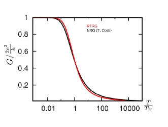
Figure 22: Comparism of the linear conductance as function of temperature from RTRG-FS (red curve) with NRG results from Costi costi . The Kondo temperature $T_{K}$ is defined such that $G(T=T_{K})={1\over 2}G_{0}$.

6 Summary and outlook

In this paper we have presented a formally exact renormalization group scheme to analyse the time evolution and the stationary state for a generic problem of dissipative quantum mechanics: An arbitrary local quantum system with a small number of states coupled to several grandcanonical reservoirs at different temperatures and chemical potentials. The RG scheme is set up by an expansion in the system-reservoir coupling using a compact diagrammatic representation which is based on a quantum field-theoretical formulation in Liouville space. It allows for a direct determination of the irreducible kernel which is the dissipative part of the kinetic equation for the reduced density matrix of the local system. This kernel determines at the same time the effective Liouville operator of the local system which is fed back into the RG equations to determine the effective propagator between the vertices. The RG scheme is set up in Laplace space allowing for an analysis of the time evolution in the presence of inhomogeneous boundary conditions leading to a nonequilibrium stationary state. Generically, we have shown how to avoid the occurence of the zero eigenvalue of the effective Liouville operator in the propagator. This provides a generic proof that the RG flow is ultimatively cut off by relaxation and dephasing rates. We have shown how to calculate the average of arbitrary observables. Correlation functions can also be calculated with similiar schemes which have not been shown here.

The RG equations represent an infinite hierarchy of coupled differential equations for effective vertices with an arbitrary number of reservoir field operators. The important input of this scheme is a cutoff-dependent correlation function for the reservoirs which can be chosen arbitrarily. However, to be able to truncate the infinite hierarchy in a systematic way, we discussed several criteria how an appropriate cutoff function has to be defined. To avoid the problem of the occurence of the zero eigenvalue in the effective propagators we developed a generic two stage procedure. First one integrates out the symmetric part of the reservoir distribution function by using perturbation theory. The result is used as an input for the following continuous RG flow with a cutoff dependent antisymmetric reservoir distribution function. The antisymmetry guarantees that the zero eigenvalue can not occur in the effective propagators between the vertices. Connected with this property is the fact that only the vertices averaged over the Keldysh indices occur in the RG scheme which simplifies the calculation. For the choice of the cutoff dependence of the reservoir correlation function within the continuous RG scheme, we proposed to integrate out the poles and branch cuts in the complex plane by defining the cutoff on the imaginary frequency axis. This has three advantages. First, high energy scales are integrated out systematically providing a high-energy cutoff for the frequency integrations in the effective perturbation theory. Secondly, with respect to the real frequencies, all energy scales are considered in each step of the RG procedure so that relaxation and dephasing rates are generated from the very beginning. Third, the numerical stability of the RG flow is improved considerably because the resolvents occuring on the r.h.s. of the RG equation contain large imaginary parts in the denominator which are of the order of the cutoff parameter.

The choice of the cutoff function is particularly simple for the special case of fermionic reservoirs with a flat density of states. In this case, the cutoff is defined by integrating out the Matsubara poles of the Fermi functions step by step. All integrations over the real frequencies can then be calculated analytically and the RG scheme can be set up on the Matsubara axis similiar to exact RG schemes for equilibrium problems. However, no analytic continuation to real frequencies is necessary to calculate transport properties. Furthermore, one has to consider a whole set of Matsubara axis shifted by the real part of the Laplace variable (to account for the time evolution) and by multiples of the chemical potentials of the reservoirs (to account for finite bias voltages). For different temperatures, each reservoir defines its own Matsubara axis. We have shown that the stability of the RG flow is expected to be very good because all imaginary parts in the denominators of the resolvents are strictly positive so that no cancellations can occur. From the real part of the denominators one can generically see that enhanced renormalizations are expected if the resonance condition $E-\bar{\mu}_{1\dots n}-h=0$ is fulfilled, where $E$ is the real part of the Laplace variable, $\bar{\mu}_{1\dots n}$ consists of the sum of arbitrary multiples of the chemical potentials of the reservoirs, and $h$ are the renormalized oscillation frequencies of the time evolution of the reduced density matrix of the local quantum system (e.g. magnetic field, level spacing, charging energy, etc.).

For the case of fermionic reservoirs with a flat density of states we have shown how to solve the RG equations analytically in the weak coupling regime. Following Ref. reininghaus_hs_preprint , we considered a system with generic spin and/or orbital fluctuations and derived the final result for the effective Liouvillian and the average of an arbitray observable up to order $J_{c}^{2}$. Here, $J_{c}$ is the order of magnitude of the effective vertex in leading order at scale $\Lambda_{c}=\mbox{Max}\{|E|,|\bar{\mu}_{1\dots n}|,|h|\}$. For the effective oscillation frequencies we found a logarithmic term $\sim\ln(\Lambda_{c}/|E-\bar{\mu}_{1\dots n}-h+i\Gamma|)$, where $\Gamma$ is the relaxation or dephasing rate corresponding to the oscillation frequency $h$. At resonance $E-\bar{\mu}_{1\dots n}-h=0$, the logarithmic term is cut off by $\Gamma$ and an enhancement $\sim J_{c}^{2}\ln(J_{c})$ is obtained. In arbitrary order one expects enhancements $\sim J_{c}^{k}(\ln{J_{c}})^{k-1}$ with $k\geq 2$. As shown in Ref. reininghaus_hs_preprint , similiar features are generically expected for the relaxation and dephasing rates and for averages of observables like the current, but the order of magnitude is one power less in $J_{c}$, i.e. one expects enhancements $\sim J_{c}^{k}(\ln{J_{c}})^{k-2}$ with $k\geq 3$ at resonance. For the special case of the nonequilibrium Kondo model at finite voltage $V$, this leads to the well-known logarithmic enhancements $\sim J_{c}^{3}\ln(V/|V-h+i\Gamma|)$ for the differential conductance at $V\sim h$ glazman_pustilnik_05 ; rosch_kroha_woelfle_PRL01 ; rosch_paaske_kroha_woelfle_PRL03 .

For strong coupling no systematic truncation scheme can be developed but we have shown that the presence of effective relaxation and dephasing rates cuts off the RG flow such that the coupling vertices will not diverge and stay of order one when the cutoff reaches the scale of the Kondo temperature (where usual poor man scaling equations diverge). We proposed a minimal set of RG equations for the strong coupling regime by truncating the RG equations and using a leading-order parametrization of the vertices. Preliminary results have been presented for the isotropic Kondo model, where a comparism to numerical renormalization group methods showed a promising coincidence for the linear conductance as function of temperature. However, within the lowest order approximation scheme, the RG equations showed an instability against exponentially small changes in the initial condition for the relaxation rate $\Gamma$. Therefore, a fitting procedure was necessary to fix the conductance at $T=V=0$ to the universal value. It remains an interesting subject for future research to include higher-order terms and study the stability of the RG equations against the choice of the initial conditions in the strong coupling regime in more detail.

Besides the strong coupling regime interesting open questions for the future concern especially the study of charge fluctuations, the time evolution, frequency-dependent density of states and bosonic systems. Especially for systems where the density of states has branch cuts in the upper half of the complex plane which do not coincide with the Matsubara axis, the RG equations get a different structure compared to fermionic systems with a flat density of states. Although the cutoff can be always defined by cutting off the imaginary part of all branch cuts, the presence of several branch cuts changes the result of the integration over the real frequencies. As a consequence, not all resolvents of the RG equations will contain the cutoff and the numerical stability of the equations has to be studied in more detail. However, the general two stage procedure and the systematic solution in the weak coupling regime can be used as well. Interesting systems in this connection are bosonic systems with particle number conservation (e.g. cold atom gases), where the condition $\omega>0>\mu_{\alpha}$ has to be fulfilled for the reservoir energies, or superconducting reservoirs where the density of states has a gap. Systems, where the frequency dependence of the density of states is analytic (besides possible poles lying at very high energies) or when the branch cuts can be turned into the lower half of the complex plane, can be described by RG equations with a similiar structure as the one for a flat density of states. The only difference is that the first step of the RG flow, where the symmetric part of the distribution function is integrated out, has to be considered again because the frequency integrals are different.

7 Acknowledgments

For the development and application of nonequilibrium RG methods I owe special thanks to S. Jakobs, M. Keil, T. Korb, J. König, V. Meden, M. Pletyukhov, and F. Reininghaus. Useful discussions are acknowledged with T. Costi, L. Glazman, S. Kehrein, H. Kroha, M. Kurz, J. Paaske, A. Rosch, D. Schuricht, M. Wegewijs, and P. Woelfle. Finally, I would like to acknowledge the support from the DFG-Forschergruppe 723 on “Functional Renormalization Group in Correlated Fermion Systems” and thank all members of this group for many fruitful discussions on general aspects of renormalization group, especially to H. Gies, W. Metzner, J. Pawlowski, M. Salmhofer, and K. Schönhammer.

Appendix A Appendix: Commutation of dot and reservoir operators

In this appendix we prove that all signs occuring from interchanges of fermionic dot and reservoir operators cancel exactly the signs emerging from the prefactor $\eta_{1}\dots\eta_{n}$ and the reversed sequence $:a_{n}\dots a_{1}:$ (compared to $:a_{1}\dots a_{n}:$) in the form (31) of the coupling

$$V\,=\,{1\over n!}\,\eta_{1}\dots\eta_{n}\,:a_{n}a_{n-1}\dots a_{1}:\,\,g_{12\dots n}\quad.$$ (584)

This means that after having defined the coupling vertex $g_{1\dots n}$ via this equation, one can use the simpler form (29) and consider dot and reservoir operators as commuting objects. This property can be proven for any average of a sequence of $V$-operators over the reservoir distribution $\rho_{res}$

$$\langle V(t_{1})V(t_{2})\dots V(t_{r})\rangle_{\rho_{res}}\quad,$$ (585)

where $V(t)$ is the interaction picture with respect to $H_{res}+H_{S}$. These are the expressions which occur for the dynamics of the reduced density matrix of the dot. For observables one of the $V$-operators is replaced by the observable but the proof remains the same since the observable is of the same form as $V$.

We start the proof for $n=1$. The coupling is of the form $V=\eta_{1}a_{1}g_{1}$ and (585) becomes (time-dependence not indicated)

$$\eta_{1}\eta_{2}\dots\eta_{r}\langle a_{1}g_{1}\,a_{2}g_{2}\dots a_{r}g_{r}\rangle_{\rho_{res}}\quad.$$ (586)

This average is only nonzero if $r$ is even and if $\sum_{i}\eta_{i}=0$, so that an equal number of annihilation and creation operators is present. Thus, taking all reservoir field operators to the right (starting with $a_{r}$), we get a total sign $(-1)^{r/2}$ from commuting them through the dot operators, and (586) reads

$$\eta_{1}\eta_{2}\dots\eta_{r}\,(-1)^{r/2}\,g_{1}g_{2}\dots g_{r}\,\langle a_{1}a_{2}\dots a_{r}\rangle_{\rho_{res}}\quad.$$ (587)

Using $\sum_{i}\eta_{i}=0$ and $r$ even, we get $\eta_{1}\dots\eta_{r}\,(-1)^{r/2}=(-1)^{r/2}(-1)^{r/2}=(-1)^{r}=1$ for the prefactor, and all sign factors have cancelled leaving an independent product of dot and reservoir operators.

For $n>1$, we formally imagine $g_{1\dots n}$ to consist of a product $g_{1}g_{2}\dots g_{n}$ of fermionic dot operators $g_{i}$ (which is allowed to determine the fermionic sign factors). From the proof for $n=1$, we know that if $V$ is of the form

$$V\,=\,{1\over n!}\,\eta_{1}\eta_{2}\dots\eta_{n}\,:(a_{1}g_{1})(a_{2}g_{2})\dots(a_{n}g_{n}):\quad,$$ (588)

all sign factors cancel in the end. Moving all reservoir field operators in (588) to the left (starting with $a_{n}$), each time involving an even number of permutations of fermionic operators, we obtain

$$V\,=\,{1\over n!}\,\eta_{1}\eta_{2}\dots\eta_{n}\,:a_{n}a_{n-1}\dots a_{1}:\,g_{1}g_{2}\dots g_{n}\quad,$$ (589)

which is precisely of the form (584) after replacing $g_{1}\dots g_{n}$ by $g_{1\dots n}$.

Appendix B Appendix: Coupling operator in Liouville space

In this appendix we prove Eq. (75) for the coupling vertex, originally defined by (71) with $V$ given by (29), i.e. we have to prove

$$L_{V}\,=\,{1\over n!}\,[g_{1\dots n}:a_{1}\dots a_{n}:\,,\cdot]_{-}\,=\,{1\over n!}\,\sigma^{p_{1}\dots p_{n}}\,G^{p_{1}\dots p_{n}}_{1\dots n}\,:J^{p_{1}}_{1}\dots J^{p_{n}}_{n}:\quad.$$ (590)

Since, due to the definition (77) of the coupling vertex, all $p_{i}$ in this expression are identical to a common index $p$, we distinguish the two cases $p=\pm$ and add them up finally. Thereby, $p=+$ produces the first term of the commutator in (590), and $p=-$ the second one.

For $p=+$, we get by acting on an arbitrary operator $A$

$$\sigma^{+\dots+}\,G^{+\dots+}_{1\dots n}\,:J^{+}_{1}\dots J^{+}_{n}:\,A\,=\,g_{1\dots n}\,:a_{1}\dots a_{n}:\,A\quad,$$ (591)

where we have used the definitions (78), (77), and (76) of the sign-operator, the coupling vertex and the reservoir field operators in Liouville space. As a consequence, the first term of the commutator in (590) is produced for $p_{i}=p=+$.

For $p=-$, we first consider bosons, where $\sigma^{-\dots-}=1$. We obtain

$$\sigma^{-\dots-}\,G^{-\dots-}_{1\dots n}\,:J^{-}_{1}\dots J^{-}_{n}:\,A\, = \,-A\,:a_{n}\dots a_{1}:\,g_{1\dots n}$$

$$= \,-A\,g_{1\dots n}\,:a_{1}\dots a_{n}:\quad,$$ (592)

coinciding with the second part of the commutator of (590).

For $p=-$ and fermions, we distinguish between $n$ even and $n$ odd. For $n$ even, we have $\sigma^{-\dots-}=(-1)^{n/2}$ and the same result is obtained for

$$\sigma^{-\dots-}\,G^{-\dots-}_{1\dots n}\,:J^{-}_{1}\dots J^{-}_{n}:\,A\, = \,-(-1)^{n/2}\,A\,:a_{n}\dots a_{1}:\,g_{1\dots n}$$

$$= \,-A\,g_{1\dots n}\,(-1)^{n/2}\,:a_{n}\dots a_{1}:\,=\,-A\,g_{1\dots n}\,:a_{1}\dots a_{n}:\quad.$$

Here we have used in the second equality the fact that operators from the reservoirs and the quantum system are considered to commute (a property which holds finally if all expressions are averaged with respect to the reservoir degrees of freedom, as explained in detail in Sec. 2.1 and appendix A). For $n$ odd, we use $\sigma^{-\dots-}=(-1)^{(n-1)/2}\sigma^{-}$, and, since $\sigma^{-}$ cancels with another $\sigma^{-}$ occuring in the definition (77) of the coupling vertex, we obtain again

$$\sigma^{-\dots-}\,G^{-\dots-}_{1\dots n}\,:J^{-}_{1}\dots J^{-}_{n}:\,A\, = \,-(-1)^{(n-1)/2}\,A\,:a_{n}\dots a_{1}:\,g_{1\dots n}$$

$$= \,-A\,g_{1\dots n}\,(-1)^{(n-1)/2}\,:a_{n}\dots a_{1}:\,=\,-A\,g_{1\dots n}\,:a_{1}\dots a_{n}:\quad,$$

and the proof of Eq. (590) is complete.

Appendix C Appendix: Kernel properties

Here we prove the property (117) of the kernel $\Sigma(E)$

$$(\Sigma(E))^{c}\,=\,-\Sigma(-E^{*})\quad.$$ (593)

We use the diagrammatic representation (112) for the kernel

$$\Sigma(E)\,\rightarrow\,{1\over S}\,(\pm)^{N_{p}}\,\left(\prod\gamma\right)_{irr}\,G\,{1\over E+X_{1}-L_{S}}\,G\,\dots\,G\,{1\over E+X_{r}-L_{S}}\,G\quad,$$ (594)

and calculate the transformation $(\Sigma(E))^{c}$ using the relation $(AB)^{c}=A^{c}B^{c}$ (see (99)). With the help of the properties (94) and (96), and renaming all summation variables by $p\rightarrow-p$ and $\eta\rightarrow-\eta$, we obtain the following replacements in (594)

$$\gamma^{pp^{\prime}}_{11^{\prime}}\, \rightarrow \,\gamma^{\bar{p},\bar{p}^{\prime}}_{\bar{1}\bar{1}^{\prime}}\,=\,\pm\,\gamma^{pp^{\prime}}_{11^{\prime}}\quad,$$ (595)

$$G^{p_{1}\dots p_{n}}_{1\dots n}\, \rightarrow \,-\,\sigma^{--\dots-}\,G^{p_{1}\dots p_{n}}_{1\dots n}\quad,$$ (596)

$${1\over E-X_{i}-L_{S}}\, \rightarrow \,{1\over E^{*}+X_{i}+L_{S}}\,=\,-{1\over-E^{*}-X_{i}-L_{S}}\quad,$$ (597)

where we have used the form $(\ref{liouville_contraction})$ for the contraction and the upper (lower) sign corresponds to bosons (fermions). Note the fact that $\eta\rightarrow-\eta$ implies also $x=\eta(\omega+\mu_{\alpha})\rightarrow-x$ and, consequently, $X_{i}\rightarrow-X_{i}$. Besides a factor $\pm$ for each contraction and a sign operator $\sigma^{--\dots-}$ for each vertex (which can give rise to a minus sign only for fermions), we obtain the replacement $E\rightarrow-E^{*}$ and a total minus sign since the number of vertices is by one larger than the number of resolvents in (594). Thus, to complete the proof of (593), we have to show for fermions that the occurence of the sign operators cancels the minus sign for each contraction. To show this, we shift all sign operators through the vertices $G$ to the left by using the property (81). As a consequence, all sign operators can be taken together to a single sign operator of the form $\sigma^{--\dots-}$, where the number of minus signs in this expression corresponds to the total number $Z$ of reservoir field operators of the diagram. Since $Z=2r$ must be an even number, the total sign operator is identical to $\sigma^{--\dots-}=(-1)^{r}$ according to the definition (78). Since $r$ is precisely the number of contractions, this sign factor cancels exacly one sign for each contraction.

Appendix D Appendix: Invariance of symmetry relations

Here we show that the symmetry properties (342)-(347) are invariant under the RG flow. Obviously, they are fulfilled initially. So we assume that we can use them on the r.h.s. of the RG equations (4.3) and (4.3), and prove them for the l.h.s.

The (anti-)symmetry relations (342) and (343) follow from the diagrammatic rules stated after (4.2). Since we sum in the RG equations over all permutations of the external indices and assign a corresponding fermionic sign, the effective vertices become automatically (anti-) symmetric.

The property (344) of conservation of probability is also trivially fulfilled, since by acting with $\mbox{Tr}_{S}$ on the RG equation and summing over the external Keldysh indices, we get zero since the first vertex already fulfils this property. Note that by summing over all Keldysh indices, the first vertex is just averaged over the Keldysh indices since the contractions do not depend on the left Keldysh index.

The properties (345)-(347), originally related to the hermiticity of the Hamiltonian, follow immediately by taking the $c$-transform (defined in Eq. (93)) of the RG equations and applying a proof in analogy to the one presented in Appendix C. The only difference is that, for the vertices, the total sign operator $\sigma^{--\dots-}$, obtained from shifting all sign operators to the left using (81), contains also the minus signs from the external indices. However, by using (80), this sign operator can be split into two sign operators, one containing the minus signs from the external vertices (leading to the sign operator on the r.h.s. of the properties (345)-(347)), the other containing the minus signs from the internal vertices which cancels the signs from all the contractions, see Appendix C.

Appendix E Appendix: Leading order RG equations

Here we prove various properties for the vertices $\bar{G}^{(1)}_{11^{\prime}}$, $\tilde{G}^{(1)}_{11^{\prime}}$, and $\bar{G}^{(2)}_{11^{\prime}}$, together with corresponding properties for the vertices $\bar{R}^{(1)}_{11^{\prime}}$ and $\bar{R}^{(2)}_{11^{\prime}}$, which are needed in Sec. 4.4. For notational simplicity, we omit in the following the index $(1)$ for all vertices.

First, we prove that the RG equations (413) and (425) for the vertices $\bar{G}^{(1)}_{11^{\prime}}$ and $\tilde{G}^{(1)}_{11^{\prime}}$ are consistent with the RG equation (420) for the vertex $g_{11^{\prime}}$ using the relations (418) and (424) between $G$ and $g$. From (418) and (420) we get

$${d\over d\Lambda}G^{pp}_{11^{\prime}}\,=\,{1\over\Lambda}\,(G^{pp}_{12}G^{pp}_{\bar{2}1^{\prime}}-G^{pp}_{1^{\prime}2}G^{pp}_{\bar{2}1})\quad,$$ (598)

by simply acting on an operator and using $G_{11^{\prime}}^{pp}=-G_{1^{\prime}1}^{pp}$. Summing this equation over $p$ gives the correct RG equation for $\bar{G}_{11^{\prime}}$

$${d\over d\Lambda}\bar{G}_{11^{\prime}}\, = \,{1\over\Lambda}\,\sum_{p}\,(G^{pp}_{12}G^{pp}_{\bar{2}1^{\prime}}-G^{pp}_{1^{\prime}2}G^{pp}_{\bar{2}1})$$ (599)

$$= \,{1\over\Lambda}\,\sum_{p}\,(G^{pp}_{12}G^{pp}_{\bar{2}1^{\prime}}-G^{pp}_{1^{\prime}2}G^{pp}_{\bar{2}1}+G^{pp}_{12}G^{\bar{p}\bar{p}}_{\bar{2}1^{\prime}}-G^{\bar{p}\bar{p}}_{1^{\prime}2}G^{pp}_{\bar{2}1})$$ (600)

$$= \,{1\over\Lambda}\,\sum_{p}\,(G^{pp}_{12}\bar{G}_{\bar{2}1^{\prime}}-\bar{G}_{1^{\prime}2}G^{pp}_{\bar{2}1})$$ (601)

$$= \,{1\over\Lambda}\,(\bar{G}_{12}\bar{G}_{\bar{2}1^{\prime}}-\bar{G}_{1^{\prime}2}\bar{G}_{\bar{2}1})\quad,$$ (602)

where $\bar{p}=-p$, and we have used $G^{pp}_{12}G^{\bar{p}\bar{p}}_{\bar{2}1^{\prime}}=G^{\bar{p}\bar{p}}_{\bar{2}1^{\prime}}G^{pp}_{12}=G^{\bar{p}\bar{p}}_{1^{\prime}2}G^{pp}_{\bar{2}1}$ to arrive at (600) (note that $2$ is a summation index which can be changed to $\bar{2}$).

Multiplying (598) with $p$ and then summing over $p$ gives the RG equation for $\tilde{G}_{11^{\prime}}$

$${d\over d\Lambda}\tilde{G}_{11^{\prime}}\, = \,{1\over\Lambda}\,\sum_{p}\,(pG^{pp}_{12}G^{pp}_{\bar{2}1^{\prime}}-pG^{pp}_{1^{\prime}2}G^{pp}_{\bar{2}1}+pG^{pp}_{12}G^{\bar{p}\bar{p}}_{\bar{2}1^{\prime}}-pG^{\bar{p}\bar{p}}_{1^{\prime}2}G^{pp}_{\bar{2}1})$$ (603)

$$= \,{1\over\Lambda}\,\sum_{p}\,(pG^{pp}_{12}\bar{G}_{\bar{2}1^{\prime}}-p\bar{G}_{1^{\prime}2}G^{pp}_{\bar{2}1})$$ (604)

$$= \,{1\over\Lambda}\,(\tilde{G}_{12}\bar{G}_{\bar{2}1^{\prime}}-\bar{G}_{1^{\prime}2}\tilde{G}_{\bar{2}1})\quad,$$ (605)

and with a similiar proof we can show the same with $\bar{G}\leftrightarrow\tilde{G}$ on the r.h.s.

Next we show that the RG equation (414) for $\bar{R}^{(1)}_{11^{\prime}}$ is consistent with the RG equation (421) for the vertex $r_{11^{\prime}}$ using the relation (419) between $R$ and $r$. As usual this holds only if one acts with the trace over the quantum system from the left. Doing this and acting with the r.h.s. of (414) on an arbitrary operator $A$, we get the correct RG equation for $\bar{R}_{11^{\prime}}$

$${1\over\Lambda}\mbox{Tr}_{S}(\bar{R}_{12}\bar{G}_{\bar{2}1^{\prime}}-\bar{R}_{1^{\prime}2}\bar{G}_{\bar{2}1})A$$ (606)

$$=\,{i\over\Lambda}\mbox{Tr}_{S}(r_{12}g_{\bar{2}1^{\prime}}-r_{1^{\prime}2}g_{\bar{2}1}-g_{\bar{2}1^{\prime}}r_{12}+g_{\bar{2}1}r_{1^{\prime}2})A$$ (607)

$$=\,{i\over\Lambda}\mbox{Tr}_{S}(r_{12}g_{\bar{2}1^{\prime}}-r_{1^{\prime}2}g_{\bar{2}1}+-g_{12}r_{\bar{2}1^{\prime}}-g_{1^{\prime}2}r_{\bar{2}1})A$$ (608)

$$=\,i{d\over d\Lambda}\mbox{Tr}_{S}\,r_{11^{\prime}}A\,=\,{d\over d\Lambda}\mbox{Tr}_{S}\,\bar{R}_{11^{\prime}}A\quad.$$ (609)

For the special case of the current vertex, we prove that the ansatz (426) for the current vertex fulfils the correct RG equation. For this we need the property

$$\mbox{Tr}_{S}\,\tilde{G}_{11^{\prime}}\bar{G}_{22^{\prime}}\,=\,-\,\mbox{Tr}_{S}\,\tilde{G}_{22^{\prime}}\bar{G}_{11^{\prime}}\quad,$$ (610)

which is based on applying several times the property $\mbox{Tr}_{S}\bar{G}_{11^{\prime}}=0$ (see (85)) or

$$\mbox{Tr}_{S}\,G^{pp}_{11^{\prime}}\,=\,-\mbox{Tr}_{S}\,G^{\bar{p}\bar{p}}_{11^{\prime}}\quad,$$ (611)

with $\bar{p}=-p$. As a consequence we also get

$$\mbox{Tr}_{S}\,G^{pp}_{11^{\prime}}G^{pp}_{22^{\prime}}\,=\,-\mbox{Tr}_{S}\,G^{\bar{p}\bar{p}}_{11^{\prime}}G^{pp}_{22^{\prime}}\,=\,-\mbox{Tr}_{S}\,G^{pp}_{22^{\prime}}G^{\bar{p}\bar{p}}_{11^{\prime}}\,=\,\mbox{Tr}_{S}\,G^{\bar{p}\bar{p}}_{22^{\prime}}G^{\bar{p}\bar{p}}_{11^{\prime}}\quad,$$ (612)

and (610) can be proven in the following way

$$\mbox{Tr}_{S}\,\tilde{G}_{11^{\prime}}\bar{G}_{22^{\prime}}\, = \,\mbox{Tr}_{S}\,\sum_{pp^{\prime}}pG^{pp}_{11^{\prime}}G^{p^{\prime}p^{\prime}}_{22^{\prime}}$$ (616)

$$=\,\mbox{Tr}_{S}\,\sum_{p}pG^{pp}_{11^{\prime}}G^{pp}_{22^{\prime}}\,+\,\mbox{Tr}_{S}\,\sum_{p}pG^{pp}_{11^{\prime}}G^{\bar{p}\bar{p}}_{22^{\prime}}$$

$$=\,\mbox{Tr}_{S}\,\sum_{p}pG^{\bar{p}\bar{p}}_{22^{\prime}}G^{\bar{p}\bar{p}}_{11^{\prime}}\,+\,\mbox{Tr}_{S}\,\sum_{p}pG^{\bar{p}\bar{p}}_{22^{\prime}}G^{pp}_{11^{\prime}}$$

$$=\,\mbox{Tr}_{S}\,\sum_{p}pG^{\bar{p}\bar{p}}_{22^{\prime}}\bar{G}_{11^{\prime}}\,=\,-\mbox{Tr}_{S}\,\sum_{p}pG^{pp}_{22^{\prime}}\bar{G}_{11^{\prime}}\,=\,-\mbox{Tr}_{S}\,\tilde{G}_{22^{\prime}}\bar{G}_{11^{\prime}}\quad,$$

where we have applied (612) in (616) and (616).

With the help of (610), we can now easily proof the correct RG equation for the current vertex using the ansatz (426)

$${d\over d\Lambda}\mbox{Tr}_{S}\,\bar{I}^{\gamma}_{11^{\prime}}\, = \,c^{\gamma}_{11^{\prime}}\mbox{Tr}_{S}\,{d\over d\Lambda}\tilde{G}_{11^{\prime}}\,=\,{1\over\Lambda}c^{\gamma}_{11^{\prime}}\mbox{Tr}_{S}\,(\tilde{G}_{12}\bar{G}_{\bar{2}1^{\prime}}-\bar{G}_{1^{\prime}2}\tilde{G}_{\bar{2}1})$$ (617)

$$= \,{1\over\Lambda}c^{\gamma}_{11^{\prime}}\mbox{Tr}_{S}\,\tilde{G}_{12}\bar{G}_{\bar{2}1^{\prime}}\,=\,{1\over\Lambda}\mbox{Tr}_{S}\,\left\{c^{\gamma}_{12}\tilde{G}_{12}\bar{G}_{\bar{2}1^{\prime}}+c^{\gamma}_{\bar{2}1^{\prime}}\tilde{G}_{12}\bar{G}_{\bar{2}1^{\prime}}\right\}$$ (618)

$$= \,{1\over\Lambda}\mbox{Tr}_{S}\,\left\{c^{\gamma}_{12}\tilde{G}_{12}\bar{G}_{\bar{2}1^{\prime}}-c^{\gamma}_{\bar{2}1^{\prime}}\tilde{G}_{\bar{2}1^{\prime}}\bar{G}_{12}\right\}$$ (619)

$$= \,{1\over\Lambda}\mbox{Tr}_{S}\,\left\{c^{\gamma}_{12}\tilde{G}_{12}\bar{G}_{\bar{2}1^{\prime}}-c^{\gamma}_{1^{\prime}2}\tilde{G}_{1^{\prime}2}\bar{G}_{\bar{2}1}\right\}$$ (620)

$$= \,{1\over\Lambda}\mbox{Tr}_{S}\,(\bar{I}^{\gamma}_{12}\bar{G}_{\bar{2}1^{\prime}}-\tilde{I}^{\gamma}_{1^{\prime}2}\bar{G}_{\bar{2}1})\quad,$$ (621)

where we have used $c^{\gamma}_{11^{\prime}}=c^{\gamma}_{12}+c^{\gamma}_{\bar{2}1^{\prime}}$ in (618) and applied (610) to arrive at (619).

We study now the RG equation for the vertices $\bar{G}^{(2)}_{11^{\prime}}$ and $\bar{R}^{(2)}_{11^{\prime}}$ which are defined by (438). For both cases we arrive with the same proof at the correct RG equation (437) in the following way (we have chosen $R$ for the proof)

$$\mbox{Tr}_{S}\,{d\over d\Lambda}\,R_{11^{\prime}}^{(2)}\, = \,-i{\pi\over 2}\mbox{Tr}_{S}\,\left\{{d\bar{R}_{12}\over d\Lambda}\tilde{G}_{\bar{2}1^{\prime}}+\bar{R}_{12}{d\tilde{G}_{\bar{2}1^{\prime}}\over d\Lambda}-(1\leftrightarrow 1^{\prime})\right\}$$ (625)

$$= \,-i{\pi\over 2\Lambda}\mbox{Tr}_{S}\,\left\{(\bar{R}_{13}\bar{G}_{\bar{3}2}-\bar{R}_{23}\bar{G}_{\bar{3}1})\tilde{G}_{\bar{2}1^{\prime}}+\right.$$

$$\hskip 56.9055pt\left.+\bar{R}_{12}(\tilde{G}_{\bar{2}3}\bar{G}_{\bar{3}1^{\prime}}-\bar{G}_{1^{\prime}3}\tilde{G}_{\bar{3}\bar{2}})-(1\leftrightarrow 1^{\prime})\right\}$$

$$= \,-i{\pi\over 2\Lambda}\mbox{Tr}_{S}\,\left\{\bar{R}_{12}(\bar{G}_{\bar{2}3}\tilde{G}_{\bar{3}1^{\prime}}-\bar{G}_{1^{\prime}3}\tilde{G}_{\bar{3}\bar{2}})+\right.$$

$$\hskip 56.9055pt\left.+\bar{R}_{13}\tilde{G}_{\bar{3}2}\bar{G}_{\bar{2}1^{\prime}}-\bar{R}_{23}\bar{G}_{\bar{3}1}\tilde{G}_{\bar{2}1^{\prime}}-(1\leftrightarrow 1^{\prime})\right\}$$

$$= {1\over\Lambda}\mbox{Tr}_{S}\,\left\{\bar{R}_{12}\bar{G}^{(2)}_{\bar{2}1^{\prime}}+\bar{R}^{(2)}_{12}\bar{G}_{\bar{2}1^{\prime}}-(1\leftrightarrow 1^{\prime})\right\}\,-$$

$$\hskip 2.84544pt-i{\pi\over 2\Lambda}\mbox{Tr}_{S}\,\bar{R}_{23}\left\{\tilde{G}_{\bar{3}1}\bar{G}_{\bar{2}1^{\prime}}-\bar{G}_{\bar{3}1}\tilde{G}_{\bar{2}1^{\prime}}-(1\leftrightarrow 1^{\prime})\right\}\quad,$$

where we have interchanged $2\leftrightarrow 3$ in the first and third term of the r.h.s. of (625) and have added and subtracted the term $\bar{R}_{23}\tilde{G}_{\bar{3}1}\bar{G}_{\bar{2}1^{\prime}}$ to (625). The first term of (625) gives the correct RG equation for $R_{11^{\prime}}^{(2)}$. The second term is zero as can be seen from

$$\bar{R}_{23}\left\{\tilde{G}_{\bar{3}1}\bar{G}_{\bar{2}1^{\prime}}-\bar{G}_{\bar{3}1}\tilde{G}_{\bar{2}1^{\prime}}-\tilde{G}_{\bar{3}1^{\prime}}\bar{G}_{\bar{2}1}+\bar{G}_{\bar{3}1^{\prime}}\tilde{G}_{\bar{2}1}\right\}$$ (626)

$$= \,\bar{R}_{23}\left\{\tilde{G}_{\bar{3}1}\bar{G}_{\bar{2}1^{\prime}}-\bar{G}_{\bar{3}1}\tilde{G}_{\bar{2}1^{\prime}}+\tilde{G}_{\bar{2}1^{\prime}}\bar{G}_{\bar{3}1}-\bar{G}_{\bar{2}1^{\prime}}\tilde{G}_{\bar{3}1}\right\}$$ (627)

$$= \,\bar{R}_{23}\sum_{pp^{\prime}}\left\{pG^{pp}_{\bar{3}1}G^{p^{\prime}p^{\prime}}_{\bar{2}1^{\prime}}-p^{\prime}G^{pp}_{\bar{3}1}G^{p^{\prime}p^{\prime}}_{\bar{2}1^{\prime}}+pG^{pp}_{\bar{2}1^{\prime}}G^{p^{\prime}p^{\prime}}_{\bar{3}1}-p^{\prime}G^{pp}_{\bar{2}1^{\prime}}G^{p^{\prime}p^{\prime}}_{\bar{3}1}\right\}$$ (628)

$$= \,2\,\bar{R}_{23}\sum_{p}\left\{pG^{pp}_{\bar{3}1}G^{\bar{p}\bar{p}}_{\bar{2}1^{\prime}}+\bar{p}G^{\bar{p}\bar{p}}_{\bar{2}1^{\prime}}G^{pp}_{\bar{3}1}\right\}$$ (629)

$$= \,2\,\bar{R}_{23}\sum_{p}p\left\{G^{pp}_{\bar{3}1}G^{\bar{p}\bar{p}}_{\bar{2}1^{\prime}}-G^{\bar{p}\bar{p}}_{\bar{2}1^{\prime}}G^{pp}_{\bar{3}1}\right\}\,=\,0\quad,$$ (630)

where we have interchanged $2\leftrightarrow 3$ in the third and fourth term of (626) and used $\bar{R}_{23}=-\bar{R}_{32}$.

Finally, we prove the properties (422) and (423). $(g_{11^{\prime}})^{\dagger}=g_{\bar{1}^{\prime}\bar{1}}$ and $(r_{11^{\prime}})^{\dagger}=r_{\bar{1}^{\prime}\bar{1}}$ follow trivially from the RG equations (420) and (421). For the vertices $\bar{G}_{11^{\prime}}$ and $\bar{R}_{11^{\prime}}$ we use the matrix representation

$$(\bar{G}_{11^{\prime}})_{s_{1}s_{1}^{\prime},s_{2}s_{2}^{\prime}}\, = \,(g_{11^{\prime}})_{s_{1}s_{2}}\delta_{s_{1}^{\prime}s_{2}^{\prime}}-\delta_{s_{1}s_{2}}(g_{11^{\prime}})_{s_{2}^{\prime}s_{1}^{\prime}}\quad,$$ (631)

$$(\bar{R}_{11^{\prime}})_{s_{1}s_{1}^{\prime},s_{2}s_{2}^{\prime}}\, = \,{i\over 2}\left\{(r_{11^{\prime}})_{s_{1}s_{2}}\delta_{s_{1}^{\prime}s_{2}^{\prime}}+\delta_{s_{1}s_{2}}(r_{11^{\prime}})_{s_{2}^{\prime}s_{1}^{\prime}}\right\}\quad,$$ (632)

and get for $\bar{G}_{11^{\prime}}^{\dagger}$

$$(\bar{G}^{\dagger}_{11^{\prime}})_{s_{1}s_{1}^{\prime},s_{2}s_{2}^{\prime}}\, = \,(\bar{G}_{11^{\prime}})^{*}_{s_{2}s_{2}^{\prime},s_{1}s_{1}^{\prime}}\,=\,(g_{11^{\prime}})^{*}_{s_{2}s_{1}}\delta_{s_{1}^{\prime}s_{2}^{\prime}}-\delta_{s_{1}s_{2}}(g_{11^{\prime}})^{*}_{s_{1}^{\prime}s_{2}^{\prime}}$$ (633)

$$= \,(g^{\dagger}_{11^{\prime}})_{s_{1}s_{2}}\delta_{s_{1}^{\prime}s_{2}^{\prime}}-\delta_{s_{1}s_{2}}(g^{\dagger}_{11^{\prime}})_{s_{2}^{\prime}s_{1}^{\prime}}$$

$$= \,(g_{\bar{1}^{\prime}\bar{1}})_{s_{1}s_{2}}\delta_{s_{1}^{\prime}s_{2}^{\prime}}-\delta_{s_{1}s_{2}}(g_{\bar{1}^{\prime}\bar{1}})_{s_{2}^{\prime}s_{1}^{\prime}}$$

$$= \,(\bar{G}_{\bar{1}^{\prime}\bar{1}})_{s_{1}s_{1}^{\prime},s_{2}s_{2}^{\prime}}\quad,$$

which proves (422). In the same way one proves (422) for the vertex $\bar{R}_{11^{\prime}}$.

References

- (1) H. Schoeller and J. König, Phys. Rev. Lett. 84, (2000) 3686.
- (2) M. Keil and H. Schoeller, Phys. Rev. B 63, (2001) 180302(R).
- (3) H. Schoeller, in Low-Dimensional Systems (T. Brandes, Lect. Notes Phys., Springer, 2000) p. 137.
- (4) T. Korb, F. Reininghaus, H. Schoeller, and J. König, Phys. Rev. B 76, (2007) 165316.
- (5) S. G. Jakobs, V. Meden, and H. Schoeller, Phys. Rev. Lett. 99, (2007) 150603.
- (6) U. Weiss, Quantum Dissipative Systems (World Scientific, Singapore, 2000); A. J. Leggett et al., Rev. Mod. Phys. 59, (1987) 1.
- (7) L. P. Kadanoff and G. Baym, Quantum Statistical Mechanics (Benjamin, New York, 1962); J. Rammer and H. Smith, Rev. Mod. Phys. 58, (1986) 323.
- (8) G. Baym and C. Pethick, in The Physics of Liquid and Solid Helium (K. H. Bennemann and J. B. Ketterson, Part II, Wiley, 78) p. 1.
- (9) D. Goldhaber-Gordon et al., Nature 391, (1998) 156; S.M. Cronenwett et al., Science 281, (1998) 540; F. Simmel et al., Phys. Rev. Lett. 83, (1999) 804; J. Nygard, D. H. Cobden, and P. E. Lindelof, Nature 408, (2000) 342; M. R. Buitelaar et al., Phys. Rev. Lett. 88, (2002) 156801; J. Park et al., Nature 417, (2002) 722.
- (10) L. I. Glazman and M. E. Raikh, Sov. Phys. JETP Lett. 47, (1988) 452; T. K. Ng and P. A. Lee, Phys. Rev. Lett. 61, (1988) 1768.
- (11) C. L. Kane and M. P. A. Fisher, Phys. Rev. B 46, (1992) 15233.
- (12) R. Landauer, IBM J. Res. Dev. 1, (1957) 223; M. Büttiker, Phys. Rev. Lett. 57, (1986) 1761; Phys. Rev. 46, (1992) 12485; Y. Imry, in Directions in Condensed Matter Physics (G. Grinstein and G. Mazenko, World Scientific, Singapore, 1986) p.101.
- (13) A. Daley, C. Kollath, U. Schollwöck, and G. Vidal, J. Stat. Mech.: Theor. Exp. (2004) P04005; S. R. White, and A. Feiguin, Phys. Rev. Lett. 93, (2004) 076401.
- (14) F. B. Anders and A. Schiller, Phys. Rev. Lett. 95, (2005) 196801.
- (15) F. B. Anders, arXiv:0802.0371.
- (16) J. E. Han and R. J. Heary, Phys. Rev. Lett. 99, (2007) 236808.
- (17) S. Weiss, J. Eckel, M. Thorwart, and R. Egger, Phys. Rev. B 77, (2008) 195316.
- (18) P. Mehta and N. Andrei, Phys. Rev. Lett. 96, (2006) 216802; ibid., Erratum cond-mat/0703246; E. Boulat and H. Saleur, Phys. Rev. B 77, (2008) 033409.
- (19) C. Caroli, R. Combescot, P. Nozieres, and D. Saint-James, J. Phys. C 5, (1972) 21.
- (20) A. P. Jauho, in Progress in Nonequilibrium Green’s Functions (M. Bonitz, World Scientific, Singapore, 2000) p. 250.
- (21) S.E. Barnes, J. Phys. F: Metal Phys. 6, (1976) 1375; P. Coleman, Phys. Rev. B 29, (1984) 3035; ibid., Phys. Rev. B 35, (1987) 5072.
- (22) S.E. Barnes, J. Phys. F: Metal Phys. 7, (1977) 2637.
- (23) N. S. Wingreen and Y. Meir, Phys. Rev. B 49, (1994) 11040.
- (24) J. Paaske, A. Rosch, H. Kroha, and P. Woelfle, Phys. Rev. B 70, (2004) 155301.
- (25) E. Fick and G. Sauermann, The Quantum Statistics of Dynamic Processes (Springer Series in Solid-State Sciences 86, Springer-Verlag, Berlin, 1990); C. W. Gardiner, Quantum Noise (Springer Series in Synergetics 56, Springer-Verlag, Berlin, 1991).
- (26) M. Grifoni, M. Sassetti, and U. Weiss, Phys. Rev. E 53, (1996) R2033.
- (27) H. Schoeller, in Mesoscopic Electron Transport (L. L. Sohn, L. P. Kouwenhoven, and G. Schön, Kluwer 1997) p. 291.
- (28) H. Schoeller and G. Schön, Phys. Rev. B 50, (1994) 18436.
- (29) J. König, H. Schoeller, and G. Schön, Europhys. Lett. 31, (1995) 31.
- (30) J. König, J. Schmid, H. Schoeller, and G. Schön, Phys. Rev. B 54, (1996) 16820.
- (31) A.C. Hewson, The Kondo Problem to Heavy Fermions (Cambridge University Press, 1993).
- (32) P. W. Anderson, J. Phys. C 3, (1970) 2436; F. D. M. Haldane, Phys. Rev. Lett. 40, (1978) 416.
- (33) E. Sela, H. S. Sim, Y. Oreg, M. E. Raikh, and F. von Oppen, Phys. Rev. Lett. 100, (2008) 056809.
- (34) P. Coleman, C. Hooley, and O. Parcollet, Phys. Rev. Lett. 86, (2001) 4088.
- (35) A. Kaminski, Yu. V. Nazarov, and L. I. Glazman, Phys. Rev. B 62, (2000) 8154.
- (36) A. Rosch, H. Kroha, and P. Woelfle, Phys. Rev. Lett. 87, (2001) 156802.
- (37) J. König and H. Schoeller, Phys. Rev. Lett. 81, (1998) 3511.
- (38) T. Pohjola, J. König, H. Schoeller, and G. Schön, Phys. Rev. B 59, (1999) 7579.
- (39) H. Schoeller, J. König, F. Kuczera, and G. Schön, J. Low Temp. Phys 118, (2000) 409.
- (40) D. Boese, W. Hofstetter, and H. Schoeller, Phys. Rev. B 64, (2001) 125309.
- (41) M. Keil and H. Schoeller, Phys. Rev. B 62, (2000) 2990.
- (42) M. Keil and H. Schoeller, Phys. Rev. B 66, (2002) 155314.
- (43) H. Schoeller and F. Reininghaus, preprint.
- (44) T. Korb, private communication.
- (45) A. Rosch, J. Paaske, H. Kroha, and P. Woelfle, Phys. Rev. Lett. 90, (2003) 076804; ibid., J. Phys. Soc. Jpn. 74, (2005) 118.
- (46) J. Paaske, A. Rosch, and P. Woelfle, Phys. Rev. B 69, (2004) 155330.
- (47) L. I. Glazman and M. Pustilnik, in Nanophysics: Coherence and Transport (H. Bouchiat et al., Elsevier, 2005) p. 427.
- (48) S. Kehrein, Phys. Rev. Lett. 95, (2005) 056602.
- (49) F. Wegner, Ann. Phys. (Leipzig) 3, (1994) 77; S. D. Glazek and K. G. Wilson, Phys. Rev. D 48, (1993) 5863; ibid., 49, (1994) 4214.
- (50) C. Wetterich, Phys. Lett. B 301, (1993) 90.
- (51) M. Salmhofer, Commun. Math. Phys. 194, (1998) 249.
- (52) R. Gezzi, T. Pruschke, and V. Meden, Phys. Rev. B 75, (2007) 045324.
- (53) S. Jakobs, diploma thesis, Aachen 2003.
- (54) S. Jakobs, M. Pletyukhov, and H. Schoeller, preprint.
- (55) A. Mitra, S. Takei, Y.B. Kim, and A.J. Millis, Phys. Rev. Lett. 97, (2006) 236808.
- (56) J. Berges, Nucl. Phys. A 699, (2002) 847.
- (57) T. Gasenzer and J. M. Pawlowski, arXiv:0710.4627v2.
- (58) M. Moeckel and S. Kehrein, Phys. Rev. Lett. 100, (2008) 175702.
- (59) J. Koch, M. E. Raikh, and F. von Oppen, Phys. Rev. Lett. 96, (2006) 056803.
- (60) M. Leijnse and M. R. Wegewijs, arXiv:0807.4027.
- (61) K. G. Wilson, Rev. Mod. Phys. 47, (1975) 773.
- (62) J. Polchinski, Nucl. Phys. B 231, (1984) 269.
- (63) H. Schoeller, private notes.
- (64) T. Korb, PhD thesis, Aachen 2007.
- (65) R. Kubo, M. Toda, and N. Hashitsume, Statistical Physics II (Springer, 1985).
- (66) M. Kurz, F. Reininghaus, R. Saptsov, H. Schoeller, and M. Wegewijs, in preparation.
- (67) A. Oguri, J. Phys. Soc. Jpn. 74, (2005) 110.
- (68) T. A. Costi, A. C. Hewson, and V. Zlatic, J. Phys.: Condens. Matter 6, (1994) 2519.