Wave Computation on the Hyperbolic Double Doughnut

Abstract.

We compute the waves propagating on the compact surface of constant negative curvature and genus 2. We adopt a variational approach using finite elements. We have to implement the action of the fuchsian group by suitable boundary conditions of periodic type. A spectral analysis of the wave allows to compute the spectrum and the eigenfunctions of the Laplace-Beltrami operator. We test the exponential decay due to a localized dumping and the ergodicity of the geodesic flow.

I. Introduction.

The Hyperbolic Double Doughnut $\mathbf{K}$ is the compact manifold of negative constant curvature with two holes. We can define it by the quotient of the hyperbolic Poincaré disc $\mathbf{D}$, by some Fuchsian group $\Gamma$. Alternatively, we can construct it as the quotient of the so-called Dirichlet polygon, or fundamental domain $\mathcal{F}\subset\mathbf{D}$ by a suitable relation of equivalence $\sim$ :

$$\mathbf{K}=\mathbf{D}/\Gamma=\mathcal{F}/\sim.$$

This beautiful object has many fascinating properties as regards the classical and quantum chaos (classical references are [1], [5]). Several important computational investigations of the spectrum were performed by using a stationnary method by R. Aurich and F. Steiner [4]. Moreover there has been much recent interest for the cosmological models with non trivial topology (a seminal work is the famous “Cosmic Topology” by M. Lachièze-Rey and J-P. Luminet [7]). In this context, $\mathbf{K}$ has been studied as a paradigm in [3], where a schema based on the finite differences on a euclidean grid was used to solve the D’Alembertian. In this paper we compute the solutions of the wave equations in the time domain, by using a variational method and a discretization with finite elements on very fine meshes. The domain of calculus is the Dirichlet polygon, therefore the initial Cauchy problem on the manifold without booundary $\mathbf{K}$, becomes a mixed problem on $\mathcal{F}$ and the action of the Fuchsian group is expressed as boundary conditions on $\partial\mathcal{F}$, analogous to periodic conditions. These boundary constraints are implemented in the choice of the basis of finite elements. By this way we obtain very accurate results on the transient waves. We test these results by performing a Fourier analysis of the transients waves that allows to find the first eigenvalues of the Laplace-Beltrami operator $\Delta_{\mathbf{K}}$ on $\mathbf{K}$. We compute also the solutions of the damped wave equation

$$\partial_{t}^{2}\psi-\Delta_{\mathbf{K}}\psi+a\partial_{t}\psi=0.$$

When $0\leq a\in L^{\infty}(\mathbf{K})$ and $a>0$ on $\partial\mathcal{F}$, the ergodicity of the geodesic flow assures that the geometric control condition of Rauch and Taylor [9] is satisfied. Our numerical experiments agree with their theoretical results, stating that the energy decays exponentially.

II. The Hyperbolic Double Doughnut.

In this part we describe the construction of the Hyperbolic Double Doughnut. First we recall some important properties of the 2-dimensional hyperbolic geometry. It is convenient to use the representation of the hyperbolic space by using the Poincaré disc

(II.1) $$\mathbf{D}:=\left\{(x,y)\in{\mathbb{R}}^{2},\;x^{2}+y^{2}<1\right\},$$

endowed with the metric expressed with the polar coordinates by

(II.2) $$ds_{\mathbf{D}}^{2}=\frac{4}{(1-r^{2})^{2}}\mbox{d}r^{2}+4\frac{r^{2}}{(1-r^{2})^{2}}\mbox{d}\varphi^{2}=\frac{4}{(1-x^{2}-y^{2})^{2}}[\mbox{d}x^{2}+\mbox{d}y^{2}].$$

It is useful to use the complex parametrization $z=x+iy$. We have to carefully distinguish the euclidean distance

(II.3) $$d(z,z^{\prime})=\mid z-z^{\prime}\mid,$$

and the hyperbolic distance associated with the hyperbolic metric, given by

(II.4) $$\cosh d_{H}(z,z^{\prime})=1+\frac{2|z-z^{\prime}|^{2}}{(1-|z|^{2})(1-|z^{\prime}|^{2})}.$$

We remark that

$$d(0,z)=\tanh\frac{d_{H}(0,z)}{2}$$

hence the euclidean circles centerd in $0$ are hyperbolic circles, and more generally, all the hyperbolic circles $\{z^{\prime};\;\;d_{H}(z^{\prime},z_{0})=R\}$, with $R>0$, $z_{0}\in\mathbf{D}$, are euclidean circles. The invariant measure $d\mu_{H}$ on the Poincaré disc allows to compute the area of any Lebesgue measurable subset $X\subset\mathbf{D}$ by the formula

(II.5) $$\mu_{H}(X)=\int_{X}\frac{4}{(1-|z|^{2})^{2}}\;dx\;dy,$$

in particular the hyperbolic area of a disc $D_{H}(0,R):=\{z;\;d_{H}(z,0)\leq R\}$ is :

(II.6) $$\mu_{H}(D_{H}(0,R))=4\pi\sinh^{2}\left(\frac{R}{2}\right).$$

The group of the isometries of $\mathbf{D}$ is generated by three kinds of transformations.

1. The Rotations of angle $\varphi_{0}\in{\mathbb{R}}$

   $$R_{\varphi_{0}}(z)=e^{i\varphi_{0}}z,$$

   and so $R_{\varphi_{0}}$ is defined in the $(x,y)$-coordinates by the matrix

   $$R_{\varphi_{0}}=\left(\begin{array}[]{cc}e^{i\frac{\varphi_{0}}{2}}&0\\ 0&e^{-i\frac{\varphi_{0}}{2}}\end{array}\right).$$

2. The Boosts, or Möbius transforms, associated with $\tau_{0}\in{\mathbb{R}}$ :

   $$T_{\tau_{0}}(z)=\frac{\cosh\frac{\tau_{0}}{2}z+\sinh\frac{\tau_{0}}{2}}{\sinh\frac{\tau_{0}}{2}z+\cosh\frac{\tau_{0}}{2}}$$

   expressed in $(x,y)$-coordinates by the matrix

   $$T_{\tau_{0}}=\left(\begin{array}[]{cc}\cosh\frac{\tau_{0}}{2}&\sinh\frac{\tau_{0}}{2}\\ \sinh\frac{\tau_{0}}{2}&\cosh\frac{\tau_{0}}{2}\end{array}\right).$$

   We remark that

   $$\cosh d_{H}(z,T_{\tau_{0}}(z))=1+2\frac{|z^{2}-1|^{2}}{(1-|z|^{2})^{2}}\sinh^{2}\left(\frac{\tau_{0}}{2}\right),$$

   therefore

   (II.7) $$\forall z\in]-1,1[,\;\;d_{H}(z,T_{\tau_{0}}(z))=\tau_{0}.$$

3. The Symmetry

   $$S(z)=\overline{z}.$$

Finally we recall that the geodesics of the Poincaré disc are the diameters and all the arcs of circles that intersect orthogonally the boundary of the disc.

Now we are ready to describe the double doughnut that is the quotient of the hyperbolic plane by the Fuchsian group of isometries, $\Gamma$, generated by the four transforms $g_{0},g_{1},g_{2},g_{3}$, where

(II.8) $$g_{k}\;=\;R_{k\frac{\pi}{4}}\;T_{\tau_{1}}\;R_{-k\frac{\pi}{4}}$$

with

(II.9) $$\tanh\frac{\tau_{1}}{2}=\sqrt{\sqrt{2}-1}.$$

The matrix of $g_{k}$ is given by :

(II.10) $$g_{k}=\left(\begin{array}[]{cc}1+\sqrt{2}&\sqrt{2+2\sqrt{2}}\,e^{ik\frac{\pi}{4}}\\ \sqrt{2+2\sqrt{2}}e^{-ik\frac{\pi}{4}}&1+\sqrt{2}\end{array}\right).$$

These isometries $g_{k}$ satisfy the relation :

(II.11) $$(g_{0}g_{1}^{-1}g_{2}g_{3}^{-1})(g_{0}^{-1}g_{1}g_{2}^{-1}g_{3})\;=\;I_{d}.$$

The Hyperbolic Double Doughnut is the quotient manifold

(II.12) $$\mathbf{K}:=\mathbf{D}/\Gamma,$$

endowed with the hyperbolic metric $ds_{\mathbf{K}}^{2}$ induced by $ds_{\mathbf{D}}^{2}$ . We know, see e.g. [1], [2], [5], that $\mathbf{K}$ is a two dimensional $C^{\infty}$ compact manifold, without boundary, its sectional curvature is constant, equal to $-1$, and its genus, that is the number of “holes”, is 2. The geodesic flow is very chaotic : it is ergodic, mixing (theorems by G.Hedlung, E. Hopf), Anosov and Bernouillian (D. Ornstein, B. Weiss).

To perform the computations of the waves on the doughnut, it is very useful to represent it by a minimal subset $\mathcal{F}\subset\mathbf{D}$ and a relation of equivalence $\sim$ such that

(II.13) $$\mathbf{K}=\mathcal{F}/\sim.$$

When $\mathcal{F}$ is choosen as small as possible, it is called Fundamental Polygon. We take

(II.14) $$\mathcal{F}:=\left\{z\in\mathbf{D};\;\;\forall i=0,...,3,\;|g_{i}(z)|\geq|z|,\;\;|g_{i}^{-1}(z)|\geq|z|\right\}.$$

We can see that $\mathcal{F}$ is a closed regular hyperbolic octogon, of which the boundary $\partial\mathcal{F}$ is the union of eight arcs of circle, that are parts of geodesics of $\mathbf{D}$. We denote $P_{j}$, $j\in{\mathbb{Z}}_{8}$, the tops of $\mathcal{F}$, and $\wideparen{P_{j}P_{j+1}}$ the eight wedges. The action of $\Gamma$ on the boundary is described by :

(II.15) $$\begin{array}[]{lllllll}P_{1}&=&g_{3}(P_{6}),&&P_{5}&=&g_{3}^{-1}(P_{2}),\\ P_{2}&=&g_{2}(P_{7}),&&P_{6}&=&g_{2}^{-1}(P_{3}),\\ P_{3}&=&g_{1}(P_{8}),&&P_{7}&=&g_{1}^{-1}(P_{4}),\\ P_{4}&=&g_{0}(P_{1}),&&P_{8}&=&g_{0}^{-1}(P_{5}),\end{array}$$

and

(II.16) $$\begin{array}[]{lllllll}\wideparen{P_{1}P_{2}}&=&g_{3}(\wideparen{P_{6}P_{5}}),&&\wideparen{P_{2}P_{3}}&=&g_{2}(\wideparen{P_{7}P_{6}}),\\ \wideparen{P_{3}P_{4}}&=&g_{1}(\wideparen{P_{8}P_{7}}),&&\wideparen{P_{4}P_{5}}&=&g_{0}(\wideparen{P_{1}P_{8}}).\end{array}$$

Figure 1. The Fundamental Domain $\mathcal{F}$.

We define the relation $\sim$ by specifying the classes of equivalence $\dot{z}$ of any $z\in\mathcal{F}$, $\dot{z}:=\Gamma(\{z\})\cap\mathcal{F}$, i.e.

(II.17) $$z\in\stackrel{{\scriptstyle\circ}}{{\mathcal{F}}}\Rightarrow\dot{z}=\{z\},$$

(II.18) $$\dot{P_{j}}=\{P_{1},\,P_{2},\;P_{3},\;P_{4},\;P_{5},\;P_{6},\;P_{7},\;P_{8}\},$$

(II.19) $$z\in\partial\mathcal{F}\setminus\dot{P_{j}}\Rightarrow\dot{z}=\{z,z_{equiv}\},$$

where according (II.16)

(II.20) $$z\in\wideparen{P_{i}P_{j}},\;\;\wideparen{P_{k}P_{l}}=g_{a}^{\pm 1}\left(\wideparen{P_{i}P_{j}}\right)\Rightarrow z_{equiv}=g_{a}^{\pm 1}(z)\in\wideparen{P_{k}P_{l}}.$$

We give some metric relations. We denote $P=\wideparen{P_{1}P_{8}}\cap{\mathbb{R}}^{-}$, $P^{\prime}=g_{0}(P)=T_{\tau_{1}}(P)$. We have

$$d_{H}(P,P^{\prime})=2d_{H}(O,P^{\prime})=\tau_{1},$$

and so

(II.21) $$\wideparen{P_{1}P_{8}}\subset\left\{z;\;\left(x+\sqrt{\frac{1+\sqrt{2}}{2}}\right)^{2}+y^{2}=\frac{\sqrt{2}-1}{2}\right\},$$

and by using the rotations we also have :

$$d_{H}(P_{i},P_{i+1})=\tau_{1}=2d_{H}(P,P_{1})=2d_{H}(O,P),$$

$$d_{H}(O,P_{i})=\tau_{2}\quad\mbox{with}\quad\tanh\frac{\tau_{2}}{2}=2^{-\frac{1}{4}},\;\;d(O,P_{i})=2^{-\frac{1}{4}}.$$

Finally the area of the fundamental domain is $\mu_{H}(\mathcal{F})=4\pi$.

III. The Waves on the Doughnut.

The Laplace Beltrami operator associated with a metric $g$, is defined by

$$\frac{1}{\sqrt{|g|}}\partial_{\mu}g^{\mu\nu}\sqrt{|g|}\partial_{\nu},\;\;g^{-1}=(g^{\mu\nu})\;,\qquad|g|=|\det g_{\mu\nu}|.$$

We consider the lorentzian manifold ${\mathbb{R}}_{t}\times\mathbf{K}$ endowed with the metric

(III.1) $$g_{\mu\nu}dx^{\mu}dx^{\nu}=dt^{2}-ds_{\mathbf{K}}^{2}.$$

We study the covariant wave equation

(III.2) $$\partial_{t}^{2}\psi-\Delta_{\mathbf{K}}\psi=0,\;\;$$

and more generally, the damped wave equation

(III.3) $$\partial_{t}^{2}\psi-\Delta_{\mathbf{K}}\psi+a\partial_{t}\psi=0,\;\;$$

whith $0\leq a\in L^{\infty}(\mathbf{K})$. Here $\Delta_{\mathbf{K}}$ is the Laplace Beltrami operator on $\mathbf{K}$. Since $\mathbf{K}$ is a smooth compact manifold without boundary, $\mathbf{K}$ endowed with its natural domain $\{u\in L^{2}(\mathbf{K});\;\;\Delta_{\mathbf{K}}u\in L^{2}(\mathbf{K})\}$ is self-adjoint and the global Cauchy problem is well posed in the framework of the finite energy spaces. Given $m\in{\mathbb{N}}$, we introduce the Sobolev space

(III.4) $$H^{m}(\mathbf{K}):=\left\{u\in L^{2}(\mathbf{K}),\;\nabla_{H}^{\alpha}u\in L^{2}(\mathbf{K}),\;\mid\alpha\mid\leq m\right\}$$

where $\nabla_{H}$ are the covariant derivatives. We can also interpret this space as the set of the distributions $u\in H^{m}_{loc}(\mathbf{D})$ such that $u\circ g=u$ for any $g\in\Gamma$. Then for all $\psi_{0}\in H^{1}(\mathbf{K})$, $\psi_{1}\in L^{2}(\mathbf{K})$, there exists a unique $\psi\in C^{0}\left({\mathbb{R}}^{+}_{t};H^{1}(\mathbf{K})\right)\cap C^{1}\left({\mathbb{R}}^{+}_{t};L^{2}(\mathbf{K})\right)$ solution of (III.3) satisfying

(III.5) $$\psi(t=0)=\psi_{0},\;\;\partial_{t}\psi(t=0)=\psi_{1},$$

and we have

(III.6) $$\int_{\mathbf{K}}\mid\partial_{t}\psi(t)\mid^{2}+\mid\nabla_{H}\psi(t)\mid^{2}d\mu_{H}+\int_{0}^{t}\int_{\mathbf{K}}a\mid\partial_{t}\psi(t)\mid^{2}d\mu_{H}dt=Cst.$$

To perform the numerical computation of this solution, we take the fundamental polygon as the domain of calculus. Then the Cauchy problem on ${\mathbb{R}}_{t}\times\mathbf{K}$ is equivalent to the mixed problem

(III.7) $$\partial_{tt}\psi-\frac{(1-x^{2}-y^{2})^{2}}{4}\left[\frac{}{}\partial_{xx}\psi+\partial_{yy}\psi\right]+a(x,y)\partial_{t}\psi=0,\;\;(t,x,y)\in{\mathbb{R}}^{+}\times\mathcal{F},$$

with the boundary conditions

(III.8) $$\forall(t,z)\in{\mathbb{R}}\times\partial\mathcal{F},\;\;z\sim z^{\prime}\Rightarrow\psi(t,z)=\psi(t,z^{\prime}).$$

We denote $H^{m}(\mathcal{F})=\{u\in L^{2}(\mathcal{F}),\;\;\forall\alpha\in{\mathbb{N}}^{2},\;\;\mid\alpha\mid\leq m,\;\;\partial_{x,y}^{\alpha}u\in L^{2}(\mathcal{F})\}$ the usual Sobolev space $H^{m}$ for the euclidean metric, and we introduce the spaces $W^{m}(\mathcal{F})$ that correspond to the spaces $H^{m}(\mathbf{K})$ :

(III.9) $$W^{m}(\mathcal{F}):=\left\{u|_{\mathcal{F}};\;\;u\in H^{m}_{loc}(\mathbf{D}),\;\;\forall g\in\Gamma,\;\;u\circ g=u\right\},$$

endowed with the norm

(III.10) $$\|u\|_{W^{m}}:=\|u|_{\mathcal{F}}\|_{H^{m}(\mathcal{F})}.$$

In particular, we have

(III.11) $$W^{1}(\mathcal{F})=\left\{u\in H^{1}(\mathcal{F}),\;\;z\sim z^{\prime}\Rightarrow u(z)=u(z^{\prime})\right\},$$

and for all $\psi_{0}\in W^{1}(\mathcal{F})$, $\psi_{1}\in L^{2}(\mathcal{F})$, there exists a unique $\psi\in C^{0}\left({\mathbb{R}}_{t}^{+};W^{1}(\mathcal{F})\right)\cap C^{1}\left({\mathbb{R}}_{t}^{+};L^{2}(\mathcal{F})\right)$ solution of (III.5), (III.7) and (III.8), and we have the energy estimate :

(III.12) $$\begin{split}\int_{{\mathcal{F}}}\frac{4}{(1-x^{2}-y^{2})^{2}}\mid\partial_{t}\psi(t,x,y)&\mid^{2}+\mid\partial_{x}\psi(t,x,y)\mid^{2}+\mid\partial_{y}\psi(t,x,y)\mid^{2}dxdy\\ &+\int_{0}^{t}\int_{{\mathcal{F}}}\frac{4a(x,y)}{(1-x^{2}-y^{2})^{2}}\mid\partial_{t}\psi(t,x,y)\mid^{2}dxdy=Cst.\end{split}$$

Since $a\in L^{\infty}(\mathcal{F})$ we have a result of regularity : when $\psi_{0}\in W^{2}(\mathcal{F})$, $\psi_{1}\in W^{1}(\mathcal{F})$, then $\psi\in C^{0}\left({\mathbb{R}}_{t};W^{2}(\mathcal{F})\right)\cap C^{1}\left({\mathbb{R}}_{t};W^{1}(\mathcal{F})\right)\cap C^{1}\left({\mathbb{R}}_{t};L^{2}(\mathcal{F})\right)$. In this case the mixed problem can be expressed as a variational problem : $\psi$ is solution iff for all $\phi\in W^{1}(\mathcal{F})$, we have :

$$\begin{split}\frac{d^{2}}{dt^{2}}\int_{{\mathcal{F}}}\frac{4}{(1-x^{2}-y^{2})^{2}}\psi(t,z)\phi(z)&dxdy+\frac{d}{dt}\int_{{\mathcal{F}}}\frac{4a(z)}{(1-x^{2}-y^{2})^{2}}\psi(t,z)\phi(z)dxdy\\ &-\int_{{\mathcal{F}}}\Delta_{x,y}\psi(t,z)\phi(z)dxdy=0.\end{split}$$

To invoke the Green formula, we denote $\nu(z)$ the unit outgoing normal at $z\in\partial\mathcal{F}$. We suppose that $\wideparen{P_{k}P_{l}}=g_{a}\left(\wideparen{P_{i}P_{j}}\right)$. Then for $z\in\wideparen{P_{i}P_{j}}$

$$g_{a}(\nu_{z})=-\nu_{g_{a}(z)},$$

Since $u\circ g_{a}=u$, we have for $u\in W^{2}(\mathcal{F})$

$$\partial_{\nu(z)}u(z)=g_{a}[\nu(z)].\nabla u(g_{a}(z))=-\partial_{\nu(g_{a}(z))}u(g_{a}(z)).$$

We deduce that for $u\in W^{2}(\mathcal{F})$, $v\in W^{1}(\mathcal{F})$, we have

$$\int_{\wideparen{P_{i}P_{j}}}v(z)\partial_{\nu(z)}ud\lambda(z)=-\int_{\wideparen{P_{k}P_{l}}}v(z)\partial_{\nu(z)}ud\lambda(z),$$

and therefore

$$\int_{\partial\mathcal{F}}v(z)\partial_{\nu(z)}ud\lambda(z)=0,\;\;\int_{\mathcal{F}}\Delta_{x,y}u(z)v(z)dxdy=-\int_{\mathcal{F}}\partial_{x}u\partial_{x}v+\partial_{y}u\partial_{y}vdxdy.$$

We have proved the following

Theorem III.1.

Given $\psi_{0}\in W^{2}(\mathcal{F})$, $\psi_{1}\in W^{1}(\mathcal{F})$, the solution $\psi$ of the Cauchy problem (III.3), (III.5), is the unique solution satisfying (III.5) of the variational problem

(III.13) $$\begin{split}\forall\phi\in W^{1}(\mathcal{F}),\;\;\frac{d^{2}}{dt^{2}}\int_{{\mathcal{F}}}\frac{4}{(1-\mid z\mid^{2})^{2}}\psi(t,z)\phi(z)&dxdy+\frac{d}{dt}\int_{{\mathcal{F}}}\frac{4a(z)}{(1-\mid z\mid^{2})^{2}}\psi(t,z)\phi(z)dxdy\\ &+\int_{{\mathcal{F}}}\partial_{x}\psi(t,z)\partial_{x}\phi(z)+\partial_{y}\psi(t,z)\partial_{y}\phi(z)dxdy=0.\end{split}$$

We solve this variational problem by the usual way. We take a family $V_{h}$, $0<h\leq h_{0}$, of finite dimensional vector subspaces of $W^{1}(\mathcal{F})$. We assume that

(III.14) $$\overline{\cup_{0<h\leq h_{0}}V_{h}}=W^{1}(\mathcal{F}).$$

We choose sequences $\psi_{0,h},\;\psi_{1,h}\in V_{h}$ such

$$\psi_{0,h}\rightarrow\psi_{0}\;\;in\;\;W^{1}(\mathcal{F}),\;\psi_{1,h}\rightarrow\psi_{1}\;\;in\;\;L^{2}(\mathcal{F}).$$

We consider the solution $\psi_{h}\in C^{\infty}({\mathbb{R}}_{t};V_{h})$ of

(III.15) $$\begin{split}\forall\phi_{h}\in V_{h},\;\;\frac{d^{2}}{dt^{2}}\int_{{\mathcal{F}}}\frac{4}{(1-\mid z\mid^{2})^{2}}\psi_{h}(t,z)\phi_{h}(z)&dxdy+\frac{d}{dt}\int_{{\mathcal{F}}}\frac{4a(z)}{(1-\mid z\mid^{2})^{2}}\psi_{h}(t,z)\phi_{h}(z)dxdy\\ &+\int_{{\mathcal{F}}}\partial_{x}\psi_{h}(t,z)\partial_{x}\phi_{h}(z)+\partial_{y}\psi_{h}(t,z)\partial_{y}\phi_{h}(z)dxdy=0,\end{split}$$

satisfying $\psi_{h}(0,.)=\psi_{0,h}(.)$, $\partial_{t}\psi_{h}(0,.)=\psi_{1,h}(.)$. Thanks to the conservation of the energy, this scheme is stable :

$$\forall T>0,\;\;\sup_{0<h\leq h_{0}}\sup_{0\leq t\leq T}\|\psi_{h}(t)\|_{W^{1}}+\|\frac{d}{dt}\psi_{h}(t)\|_{L^{2}}<\infty.$$

Moreover, when $\psi\in C^{2}\left({\mathbb{R}}^{+}_{t};W^{1}(\mathcal{F})\right)$, it is also converging :

$$\forall T>0,\;\;\sup_{0\leq t\leq T}\|\psi_{h}(t)-\psi(t)\|_{W^{1}}+\|\frac{d}{dt}\psi_{h}(t)-\frac{d}{dt}\psi(t)\|_{L^{2}}\rightarrow 0,\;\;h\rightarrow 0.$$

If we take a basis $\left(e_{j}^{h}\right)_{1\leq j\leq N_{h}}$ of $V_{h}$, we expand $\psi_{h}$ on this basis :

$$\psi_{h}(t)=\sum_{j=1}^{N_{h}}\psi_{j}^{h}(t)e_{j}^{h},$$

and we introduce

$${\mathbb{M}}=\left(M_{ij}\right)_{1\leq i,j\leq N_{h}},\;\;M_{ij}:=\int_{{\mathcal{F}}}\frac{4}{(1-\mid z\mid^{2})^{2}}e_{i}^{h}(z)e_{j}^{h}(z)dxdy,$$

$${\mathbb{D}}=\left(D_{ij}\right)_{1\leq i,j\leq N_{h}},\;\;D_{ij}:=\int_{{\mathcal{F}}}\frac{4a(z)}{(1-\mid z\mid^{2})^{2}}e_{i}^{h}(z)e_{j}^{h}(z)dxdy,$$

$${\mathbb{K}}=\left(K_{ij}\right)_{1\leq i,j\leq N_{h}},\;\;K_{ij}:=\int_{{\mathcal{F}}}\partial_{x}e_{i}^{h}(z)\partial_{x}e_{j}^{h}(z)+\partial_{y}e_{i}^{h}(z)\partial_{y}e_{j}^{h}(z)dxdy,$$

$$X:=\left(\begin{array}[]{c}\psi_{1}^{h}\\ \psi_{2}^{h}\\ .\\ .\\ .\\ \psi_{N_{h}}^{h}\end{array}\right).$$

Then the variational formulation is equivalent to

(III.16) $${\mathbb{M}}X^{\prime\prime}+{\mathbb{D}}X^{\prime}+{\mathbb{K}}X=0.$$

This differential system is solved very simply by iteration by solving

(III.17) $${\mathbb{M}}(X^{n+1}-2X^{n}+X^{n-1})+\frac{\Delta T}{2}{\mathbb{D}}(X^{n+1}-X^{n-1})+(\Delta T)^{2}{\mathbb{K}}X^{n}=0.$$

We know that this scheme is stable, and so convergent by the Lax theorem, when

(III.18) $$\sup_{X\neq 0}\frac{<{\mathbb{K}}X,X>}{<{\mathbb{M}}X,X>}<\frac{4}{\Delta T^{2}},$$

and if there exists $K>0$ such that

(III.19) $$\forall h\in]0,h_{0}],\;\;\forall\phi_{h}\in V_{h},\;\;\|\nabla_{x,y}\phi_{h}\|_{L^{2}(\mathcal{F})}\leq\frac{K}{h}\left\|\frac{2}{1-\mid z\mid^{2}}\phi_{h}\right\|_{L^{2}(\mathcal{F})},$$

the CFL condition

(III.20) $$K\Delta T<2h,$$

is sufficient to assure the stability and the convergence of our scheme.

IV. Numerical resolution

IV.1. Mesh

First of all we construct the boundary $\partial\mathcal{F}$ from the equation (II.21) and we perform a discretization that is equidistant for the hyperbolic metric. Next we use the mesh generators Emc2™and bamg™created by INRIA. If we only use Emc2™, the mesh contains too many vertices and is not suitable for the hyperbolic metric. So a first mesh is created by Emc2™. We also consider a circle which is uniformly discretized with the same hyperbolic step than the exterior geometry. The radius is choosen as the final mesh is almost uniform. At last, we impose on every point of the exterior and interior geometry a metric, in the sense of bamg™. This software can next create a mesh which is more uniform, with respect to the hyperbolic metric, than the first mesh, and that has a reasonnable number of vertices.

To test the uniformity of the mesh, we compute the extrema of the hyperbolic distance between two neighbor vertices. As a check of the accuracy of the meshes we evaluated the area of the polygons created by the meshes, and we compared to $4\pi$ (area of the domain). Here are some examples:

$$\begin{array}[]{lcccl}Mesh&number\ of\ vertices&\max d_{H}&\min d_{H}&area/4\pi\\ Mesh1\;:&7448&0.087&0.027&1.00012\\ Mesh2\;:&17574&0.049&0.0177&1.00007\\ Mesh3\;:&37329&0.036&0.012&1.00003\\ Mesh4\;:&67517&0.027&0.009&1.000018\\ \end{array}$$

In our meshes, the greater hyperbolic distance between consecutive vertices is not reached near the exterior boundary. To give an idea of the accuracy of this dicretization, we show in the following figure, a very rough mesh :

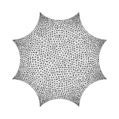
Figure 2. A very rough mesh with 1756 vertices.

IV.2. $V_{h}$ space

We construct the finite element spaces of ${\mathbb{P}}_{1}$ type. We note $\mathcal{T}_{h}$ all triangles of a mesh, and $\displaystyle{\mathcal{F}_{h}=\cup_{K\in\mathcal{T}_{h}}K}$.

$$V_{h}:=\left\{v:\mathcal{F}_{h}\rightarrow{\mathbb{R}},\;v\in\mathcal{C}^{0}(\mathcal{F}_{h}),\;\forall K\in\mathcal{T}_{h}\;v_{|K}\in{\mathbb{P}}_{1}(K),\;M\sim M^{\prime}\Rightarrow v(M)=v(M^{\prime})\right\}$$

If $M_{i}$ and $M_{j}$ denote two vertices of the mesh, we define a basis $\left(e_{j}^{h}\right)_{1\leq j\leq N_{h}}$ of $V_{h}$ by:

1. If $M_{j}\not\in\partial\mathcal{F}$ : $e_{j}^{h}(M_{i})=\delta_{ij}$

2. If $M_{j}$ is a $P_{j}$ point: $e_{j}^{h}(M_{i})=\left\{\begin{array}[]{ll}1&if\ M_{i}=P_{i}\\ 0&otherwise\end{array}\right.$

3. If $M_{j}\in\partial\mathcal{F}$, and is not a $P_{j}$ point: $e_{j}^{h}(M_{i})=\left\{\begin{array}[]{ll}1&if\ M_{i}\sim M_{j}\\ 0&otherwise\end{array}\right.$

In particular, we have to determine the equivalent points on $\partial\mathcal{F}$. To that, we write a program implementing the relations (II.20).

The number of nodes $N_{h}$ is the sum of the number of the vertices which are not in $\partial\mathcal{F}$, the number of vertices which are on four consecutive arcs of $\partial\mathcal{F}$ without beeing a $P_{i}$ point, and one (because all $P_{i}$ points are equivalent to one of them).

IV.3. Matrix form of the problem

${\mathbb{K}}(i,j)$ and ${\mathbb{M}}(i,j)$ are found with a numerical integration using the value at the middle of the edges of the triangles.

The stiffness matrix ${\mathbb{K}}$ and the mass matrix ${\mathbb{M}}$ are sparse and symetric matrices. So we choose a Morse stockage of their lower part, and all of the calculations will be performed with this stockage.

To solve the linear problem we use a preconditionned conjugate gradient method. The preconditionner is an incomplete Choleski factorisation, and the starting point is the solution obtained with a diagonal preconditionner.

IV.4. Initial data

We consider the case where the initial velocity $\psi_{1}=0$, i.e. $X^{0}=X^{1}=0$, and we choose first initial datas with a more or less small support near a given point. For instance, for the wave depicted in Figure 3, we have taken

(IV.1) $$\psi_{0}(x,y)=100e^{\frac{1}{100x^{2}+100y^{2}-1}},\;\;for\;x^{2}+y^{2}<\frac{1}{100},\;\psi_{0}(x,y)=0,\;\;for\;x^{2}+y^{2}\geq\frac{1}{100}.$$

IV.5. Discretized energy

In order to see the stability of our method we perform $E_{d}(t)$ the discretized energy at the time $t$:

$$E(n\Delta t)=\left<{\mathbb{M}}\;\frac{X^{n}-X^{n-1}}{\Delta t}\;,\;\frac{X^{n}-X^{n-1}}{\Delta t}\right>\;+\;\left<{\mathbb{K}}\;X^{n-1}\;,\;X^{n}\right>$$

It is well known that our schema is conservative when $a=0$, hence $E_{d}$ must be invariant all along the resolution. We test this property with the previous initial data.

$$\begin{array}[]{|lc|cc|}\hline\cr&E_{d}(0):&E_{d}(100):&\\ &&&\\ &&\quad\rm{with\ }\Delta t=0.001:&\quad\rm{with\ }\ \Delta t=0.0005:\\ Mesh1\;:&8455.89602005935&8455.89602005865&\\ Mesh2\;:&8484.17400988788&8484.17400988815&8484.17400988936\\ Mesh3\;:&8494.43409419468&8494.43409419464&8494.43409419511\\ Mesh4\;:&8498.39023175937&8498.39023175945&8498.39023175923\\ \hline\cr\end{array}$$

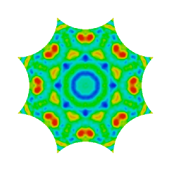
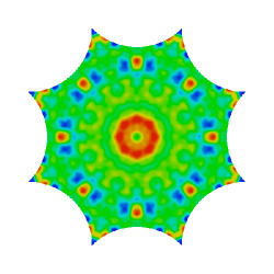
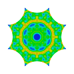
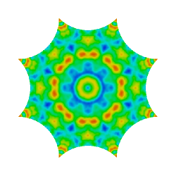
Figure 3. The transient wave at $t=34$, $t=35$, $t=36$, $t=37$.

IV.6. Eigenvalues

We test our scheme in the time domain, by looking for the eigenvalues of the hamiltonian when $a=0$. Since the Laplace-Beltrami operator $\Delta_{\mathbf{K}}$ on the Hyperbolic Double Doughnut is a non positive, self-adjoint elliptic operator on a compact manifold, its spectrum is a discrete set of eigenvalues $-q^{2}\leq 0$, and by the Hilbert-Schmidt theorem, there exists an orthonormal basis in $L^{2}(\mathbf{K})$, formed of eigenfunctions $\left(\psi_{q}\right)_{q}\subset H^{\infty}(\mathbf{K})$ associated to $q^{2}$, i.e.

(IV.2) $$-\frac{(1-x^{2}-y^{2})^{2}}{4}\left[\frac{}{}\partial_{xx}\psi_{q}+\partial_{yy}\psi_{q}\right]=q^{2}\psi_{q},\;\;\psi_{q}\in W^{\infty}(\mathcal{F}).$$

We take $\psi_{0}=\frac{1}{2\sqrt{\pi}}$. Therefore any finite energy solution $\psi(t,x,y)$ of $\partial_{t}^{2}\psi-\Delta_{\mathbf{K}}\psi=0$ has an expansion of the form $\sum_{q}e^{iqt}\psi_{q}(x,y)$ (such expansions exist also for the damped wave equation, when $a>0$, see [6]). More precisely, if we denote $<,>$ the scalar product in $L^{2}(\mathbf{K})$, we write

(IV.3) $$\begin{split}\psi(t,x,y)=&\frac{1}{4\pi}(<\partial_{t}\psi(0,.),1>t+<\psi(0,.),1>)\\ &+\sum_{q\neq 0}<\partial_{t}\psi(0,.),\psi_{q}>\frac{\sin qt}{q}\;\psi_{q}(x,y)+\;<\psi(0,.),\psi_{q}>\cos qt\;\psi_{q}(x,y).\end{split}$$

To compute the eigenvalues $q$, we investigate the Fourier transform in time of the signal $\psi(t,x,y)$ in the case where $\partial_{t}\psi(0,x,y)=0$. We fix some large $T>>1$, and we put $\Psi_{\omega}(X):=\int_{0}^{T}\psi(t,X)e^{i\omega t}\;dt.$ Then $\Psi_{\omega}(t)\sim CT^{2}(\omega^{2}-q^{2})^{-1}$, $T\rightarrow\infty$. Practically, during the time resolution of the equation we store the values of the solution at some points $M$, including the origin, $P^{\prime}$, $M_{0}$ near $P_{4}$, for the discrete time $k\Delta t$, $N_{i}\leq k\leq N_{f}$. We choose the initial step $N_{i}$ in order to the transient wave is stabilized, that to say $N_{i}\Delta t$ is greater than the diameter of the doughnut, i.e. $N_{i}\Delta t\geq 2*d_{H}(0,P_{i})\simeq 4.8969$. Then we compute a DFT of $(\psi_{h}(k\Delta t,M))_{N_{i}\leq k\leq N_{f}}$ with the free FFT library fftw. Let us note $(\Psi_{j}(M))_{0,N_{f}-N_{i}+1}$ the result. If $\Psi_{j}(M):=\sum_{k=0}^{N_{f}-N_{i}+1}\psi((N_{i}+k)\Delta t,x,y)e^{-(\frac{2\pi}{N_{f}-N_{i}+1}jk)i}$, we search the values $jmax_{1}$, $jmax_{2}$, … for which $(\|\Psi_{j}(M)\|^{2})_{j}$ has a maximum. Then the eigenvalues found by the algoritm expressed as:

$$q=\frac{2\pi}{(N_{f}-N_{i}+1)\Delta t}jmax$$

We have made a lot of tests by varying parameters such as: $\Delta t$, $N_{i}$, $N_{f}$, the mesh, the observation point $M$. With the initial data (IV.1), we find the following values for $q$ :

$$\begin{array}[]{cc}1,96\pm 0,02&2,85\pm 0,04\\ 4,34\pm 0,06&4,83\pm 0,06\\ 6,00\pm 0,06&6,63\pm 0,06\end{array}$$

These results agree with the results obtained with a stationnary method with a mesh of 3518 vertices in [4].
Alternatively, we could also use the power spectrum and calculate the square of the modulus of $\Psi_{\omega}(x,y)$

$$\begin{split}\|\Psi_{\omega}\|_{L^{2}(\mathbf{K})}^{2}&=\frac{1}{4\pi}\mid<\psi(0,.),1>\mid^{2}\\ &+\frac{1}{2}\sum_{q}<\psi(0,.),\psi_{q}>^{2}\left[\frac{\sin^{2}\frac{(q+\omega)T}{2}}{(q+\omega)^{2}}+\frac{\sin^{2}\frac{(\omega-q)T}{2}}{(\omega-q)^{2}}+\frac{1}{\omega^{2}-q^{2}}\left(\cos^{2}\omega T-\cos\omega T\cos qT\right)\right]\end{split}$$

Therefore, for an eigenvalue $q_{0}$:

$$\|\Psi_{\omega}\|_{L^{2}(\mathbf{K})}^{2}\geq\;<\psi(0,.),\psi_{q}>^{2}\left(\frac{T^{2}}{4}-\frac{T}{2q}\right).$$

IV.7. Damped waves

We test our scheme for the damped wave equation (III.3) when the damping function $a\geq 0$ is non zero (for deep theoretical results, see [6], [8], [9]). We know that the energy of any finite energy solution decays exponentially (uniformly with respect to the initial energy) iff the dumping $a$ satisfies the assumption of geometric control introduced by J. Rauch and M. Taylor in [9]. This condition means

(IV.4) $$\int_{0}^{\infty}a(x(t),y(t))dt=+\infty$$

for any geodesic $(x(t),y(t))$. Since the geodesic flow on the compact Riemaniann manifold with constant negative curvature is very chaotic (more precisely ergodic, mixing, Anosov, Bernouillian see e.g. [1], [2], [5]), it is sufficient to have $a>0$ near $\partial\mathcal{F}$. Nevertheless we constat an exponential decay for some solution, even if we choose a dumping function $a$ equal to a positive constant on very small support that does not satisfy (IV.4) : $a>0$ only on one triangle and its close neighbors.

The next figures are obtained with mesh3 and $a$ defined by:

$$a(x,y)=0,\;{\rm for\ },\mid z\mid<0.6\quad;\quad a(x,y)=0.1,\;{\rm otherwise.}$$

Figure 4. Logarithm of the energy as a function of time.

Figure 5. Solution at the origin.

References

- [1] N.L. Balazs, A. Voros. Chaos on the pseudosphere. Phys. Rep., 143-3: 109-240, 1986.
- [2] M. B. Bekka, M. Mayer. Ergodic Theory and Topological Dynamics of Group Actions on Homogeneous Spaces. London Mathematical Society Lecture Notes Series, 269, Cambridge University Press, 2000.
- [3] N.J. Cornish, N.G. Turok. Ringing the eigenmodes from compact manifolds. Class. Quantum Grav., 15:2699-2710, 1998.
- [4] R. Aurich, F. Steiner. Periodic-orbit sum rules for the Hadamard-Gutzwiller model. Phys. D, 39: 169-193, 1989.
- [5] M. C. Gutzwiller. Chaos in Classical and Quantum Mechanics. Interdisciplinary Applied Mathematics, 1, Springer-Verlag, 1990.
- [6] M. Hitrik. Eigenfrequencies and expansions for damped wave equations. Methods Appl. Anal., 10,4 : 543-564, 2003.
- [7] M. Lachièze-Rey, J.P. Luminet. Phys. Rep., 254:135-214, 1995.
- [8] G. Lebeau. Equations des ondes amorties. Séminaire X-EDP, 15, Ecole Polytechnique, 1994.
- [9] J. Rauch, M. Taylor. Decay of solutions to nondissipative hyperbolic systems on compact manifolds. Comm. pure Appl. Math., 28:501-523, 1975.