Neutral triplet Collective Mode as a new decay channel in Graphite

Abstract

In an earlier work we predicted the existence of a neutral triplet collective mode in undoped graphene and graphite [Phys. Rev. Lett. 89 (2002) 016402]. In this work we study a phenomenological Hamiltonian describing the interaction of tight-binding electrons on honeycomb lattice with such a dispersive neutral triplet boson. Our Hamiltonian is a generalization of the Holstein polaron problem to the case of triplet bosons with non-trivial dispersion all over the Brillouin zone. This collective mode constitutes an important excitation branch which can contribute to the decay rate of the electronic excitations. The presence of such collective mode, modifies the spectral properties of electrons in graphite and undoped graphene. In particular such collective mode, as will be shown in this paper, can account for some part of the missing decay rate in a time-domain measurement done on graphite.

I introduction

Recently Novoselov and coworkers have been able to fabricate graphene, a single atomic layer of graphite Novoselov . This discovery has brought graphene to the center of attention of many researchers NetoRMP . The fundamental difference of the electronic spectrum of graphene with respect to the usual metals is the existence of Fermi points around which an effective Dirac theory describes the electronic states semenoff . The suspended graphene now can be fabricated in which the effects of impurity and substrate is substantially reduced and one can approach the ballistic limit of transport with Dirac electrons AnderiNanotech2007 .

Starting from a single layer of graphene, and adding further layers, one obtains, graphene multi-layers. For few layers the even-odd effects due to quantum confinement arise NetoRMP . However, as the number of layers exceeds $\sim 10$, one approaches the bulk limit, or graphite. The Dirac part of the energy dispersion of graphite is qualitatively similar to graphene SaitoBook . The only important difference between the electronic states of graphite and graphene is the presence of small pockets up to $\sim 40$ meV, beyond which the Dirac description applies to low-energy physics of graphite as well Kopeldhv ; LanzaraGraphite . Ignoring such pockets which originate from the weak interlayer coupling, the electronic structure of bulk graphite can be approximately described by a tight binding model on a 2D honeycomb lattice. In our approach both highly oriented pyrolitic graphite (HOPG) as well as undoped graphene are treated within this model. The calculations of this paper is aimed to explain the life-time anomaly in HOPG, but applies to undoped graphene as well.

The presence of Dirac points makes the nature of particle-hole excitations in graphene, drastically different from systems possessing extended Fermi surface. Due to such cone like spectrum, there will be a region below the particle-hole continuum, where no particle-hole pairs can exist. Such a ”window” does not exist in usual metals baskaranjafari . A simple random phase approximation (RPA) analysis shows that presence of such window below the particle-hole continuum, provides a unique opportunity for existence of a triplet bound state of electron-hole excitation baskaranjafari . An intuitive way to understand such a triplet electron-hole bound state is to view the semi-metallic graphene from semiconducting side. From this point of view, such collective excitation can be regarded as analogue of triplet excitons jafaribaskaran .

In this work we focus on the life time experiment done on HOPG sample which corresponds to undoped graphite. The time resolved photoemission spectroscopy (TRPES) done by Moos and coworkers moos on HOPG, was employed to measure the decay rate of quasi particles in graphite. There are two salient features of the TRPES experiment reported by Moos et. al. moos which for convenience has been included in Fig. 1: (i) The plateau in the energy range $1-2$ eV is already a marked deviation from Fermi liquid prediction which was qualitatively explained in Refs. moos ; spataru , in terms of the peculiar from of the graphite dispersion near the saddle point. Such a plateau has been reported in the carrier life time of doped graphene in angular resolved photoemission spectroscopy (ARPES) experiments as well bostwick which can be understood in terms of a similar G₀W type of treatment DasSarmaLifetime . (ii) The second important observation of the above TRPES experiment was that the decay rate of excitations in the whole range of energies over which the measurement was performed, was larger than the ab-initio calculation of Ref. spataru . This clearly means that there should be another decay channel for quasi particles, especially in the energy range $1-2$ eV. In the whole measurement range the experimentally observed decay rate is almost a factor of $2$ larger than the GW calculation.

Obviously the phonons cease to exist beyond $0.2$ eV, and hence can not be responsible for the missing decay channel in the energies reported in Ref moos . Moreover, both in HOPG and undoped graphene, there are no plasmons whatsoever HwanDasSarma . Therefore we believe this lifetime experiment already point to the existence of an unnoticed bosonic branch of neutral excitations baskaranjafari ; jafaribaskaran . There are also other evidences based on the Fermi velocity renormalization measurements: If one appeals to electron-phonon coupling to explain the experimentally observed reduction in Fermi velocity $v_{F}$ with respect to band structure prediction, one has to use an electron-phonon coupling which is almost $\sim 5$ times larger than the density functional theory estimates andrei . Therefore it seems that the phonons are not enough to account for about $20\%$ Fermi velocity renormalization andrei . The second experimental hint for the existence of such a bosonic mode, is the remarkable observation of the Bose metal-insulator transition tuned by magnetic field bosemetal .

Based on the above evidences, in this paper we employ a triplet bosonic mode predicted in Ref. baskaranjafari with a gapless dispersion up to $\omega_{\rm max}\sim 2.1$ eV. Our model is a natural generalization of the polaron problem, with spin-flip processes included. We generalize the momentum average (MA) approximation developed in the context of the polaron problem by Berciu berciu1 to take into account the spin-flip vertices as well as the nontrivial dispersion in the spectrum of bosons. First we introduce our model and the MA method. Next we apply the MA approximation to discuss the coupling of a triplet boson to electronic states of graphene quasi particles. The details of generalization of MA approximation to spin-flip processes is discussed in the appendix.

II Model and method

We start with the Hamiltonian (1) describing the tight-binding electrons on honeycomb lattice (first term), along with dispersive triplet bosons (second term) and the interaction between electrons and bosons (third term):

$$H=\sum_{\vec{k},\alpha=\uparrow,\downarrow}\epsilon_{\vec{k}}c^{{\dagger}}_{\vec{k},\alpha}c_{\vec{k},\alpha}+\sum_{\vec{q},m=\pm 1}\omega_{\vec{q}}S^{{\dagger}}_{\vec{q},m}S_{\vec{q},m}$$

$$+g\sum_{\vec{k},\vec{q},m,m^{\prime},\alpha,\alpha^{\prime}}(S^{{\dagger}}_{\vec{q},m}+S_{-\vec{q},m^{\prime}})c^{{\dagger}}_{\vec{k}-\vec{q},\alpha}c_{\vec{k},\alpha^{\prime}},$$ (1)

where $\epsilon_{\vec{k}}=\pm t\sqrt{1+\cos(\sqrt{3}k_{y}/2)\cos(k_{x}/2)+4\cos^{2}(k_{x}/2)}$ is spectrum of fermions for (conduction/valance) band and $\omega_{\vec{q}}$ describes the dispersion of spin-1 bosons baskaranjafari . Here $c^{{\dagger}}_{\vec{k},\alpha}(c_{\vec{k},\alpha})$ is creation (annihilation) operator for fermions with momentum $\vec{k}$ and spin $\alpha=\uparrow,\downarrow$ in either of the valence or conduction bands, while $S^{{\dagger}}_{\vec{q},m},S_{\vec{q},m}$ are ladder operator for spin-1 bosons with momentum $\vec{q}$, and magnetic quantum numbers $m=\pm 1,0$. In this Hamiltonian, $g$ is the coupling strength and describes how strongly the exchange of triplet excitons takes place among the electrons. Estimates of a similar coupling in doped solid C₆₀ suggests $g\sim 0.3$ for those systems BaskaranTosatti . Presence of such term, favours singlet pairing under suitable conditions BaskaranTosatti ; Shenoy .

The interaction term of the Hamiltonian (1) describes both spin flip ($m=\pm 1$) as well as non spin flip ($m=0$) processes. Since non spin flip processes can exist in presence of spin-0 bosons as well, to isolate the contribution of the spin flip processes, we focus on $m=\pm 1$ terms only. In this sector, requiring the Hamiltonian (1) to be Hermitian, gives rise to the following restrictions on possible values of $m,m^{\prime},\alpha,\alpha^{\prime}$:

$$m=1(-1)\rightarrow m^{\prime}=-1(1)\rightarrow\alpha=\downarrow(\uparrow)\rightarrow\alpha^{\prime}=\uparrow(\downarrow).$$

We use momentum average (MA) approximation to calculate the Green’s function and self-energy of system  berciu1 ; berciu2 which yields various physical quantities such as decay rate. Comparison of MA and its descendants (e.g. MA(1), MA(2), etc) with other methods demonstrated that this method is accurate for the entire spectrum (both low and high energy) and for all coupling strengths and in all dimensions berciu2 . This approximation was also used successfully for analysis of the effects of ripples on graphene sheet berciu-graphene . In the following, we use MA(1) approximation, the details of which for the case of dispersive mode with spin-1 are derived in the appendix.

The single electron Green’s function can be written as:

$$G_{\alpha,\beta}(\vec{k},\tau)=-i\theta(\tau)\langle 0|c_{\vec{k},\alpha}e^{iH\tau}c^{{\dagger}}_{\vec{k},\tau}|0\rangle,$$ (2)

where $\alpha,\beta$ are spin indices, and $|0\rangle$ is vacuum state. In the absence of bosons the free propagator is

$$G_{0}(\vec{k},\omega)=\frac{1}{\omega-\epsilon_{\vec{k}}+i\eta}.$$ (3)

To take into account the coupling to triplet bosons, we use the equation of motion for $G_{\alpha,\beta}(\vec{k},\tau)$ to obtain (see appendix),

$$G_{\alpha,\beta}(\vec{k},\omega)=G_{0}(\vec{k},\omega)[\delta_{\alpha,\beta}+\!g\!\!\sum_{\vec{q}_{1},m_{1}}\!\!F^{\alpha,-\beta}_{1}(\vec{k},\vec{q}_{1},m_{1};\omega)],$$ (4)

where

$$F^{\alpha,-\beta}_{1}(\vec{k},\vec{q}_{1},m_{1};\omega)=\langle 0|c_{\vec{k},\alpha}\frac{1}{\omega-\hat{H}+i\eta}c^{{\dagger}}_{\vec{k}-\vec{q},-\beta}S^{{\dagger}}_{\vec{q},m_{1}}|0\rangle.$$ (5)

Here, $F_{1}$ is the amplitude for the process in which the initial state contains a fermion and a boson, and the final states contains only a fermion with opposite spin. Hence, physically it corresponds to the amplitude of annihilating one triplet ($\Delta m=\pm 1$) boson. Applying again the equation of motion to $F_{1}$ generates hierarchy of equations containing amplitudes with multi-boson states:

$$F^{\alpha,-\beta}_{1}(\vec{k},\vec{q}_{1},m_{1},\omega)=$$ (6)

$$G_{0}(\vec{k}-\vec{q}_{1},\omega-\omega_{\vec{q}_{1}})[g^{2}\!+\!\!\!\sum_{\vec{q}_{2},m_{2}}\!\!F^{\alpha,\beta}_{2}(\vec{k},\vec{q}_{1},\vec{q}_{2},m_{1},m_{2};\omega)].$$

Although each internal vertex may contain spin flip scatterings, since the Hamiltonian (1) preserves the spin, the incoming and outgoing fermions must have the same spin. Hence the Green’s function (2) must be diagonal with respect to the spin indices. The rigorous proof of this is given in the appendix. Also, by Dyson equation, the self-energy is also diagonal with respect to spin indices:

$$G_{\alpha,\alpha}(\vec{k},\omega)=[\omega-\epsilon_{\vec{k}}-\Sigma^{\alpha,\alpha}(\vec{k},\omega)+i\eta]^{-1}.$$ (7)

The self-energy $\Sigma^{\alpha,\alpha}(\vec{k},\omega)$ in MA(1) approximation is given by (see appendix),

$$\Sigma^{\alpha,\alpha}(\omega)=\frac{g^{2}\sum_{\vec{k},q_{1}}G_{0}(\vec{k}-\vec{q}_{1},\omega-\omega_{\vec{q}_{1}}-g^{2}A_{1}(\omega))}{1-g^{2}\sum_{\vec{k},\vec{q}_{1}}G_{0}(\vec{k}-\vec{q}_{1},\omega-\omega_{\vec{q}_{1}}-g^{2}A_{1}(\omega))(A_{2}(\omega)-A_{1}(\omega))},$$ (8)

where $A_{1},A_{2}$ are functions of $\omega$, defined in the appendix. The self-energy contains all interaction effects, and can be used to calculate spectral weights, decay rates, etc. in a straightforward way mahan .

III Results

Now we are in position to derive decay rate or lifetime of quasi particles (QP) of HOPG/graphene in presence of spin-1 bosonic collective mode. There are some other decay mechanisms such as electron-hole spataru , electron-phonon GonzalezPerfetto , and electron-plasmon scatterings HwanDasSarma . In doped graphene, all the above mechanisms might contribute to the renormalization of QP properties. However, in HOPG graphite and undoped graphene there are no plasmons to couple to electronic degrees of freedom.

III.1 The decay rate

The imaginary part of self-energy related to life-time and decay rate of QP,

$$\frac{1}{\tau}\propto-\mbox{Im}[\mbox{Tr}{\Sigma^{\alpha,\alpha}(\vec{k},\omega)}].$$ (9)

We have numerically evaluated the integrals necessary to get the self-energy (8). In Fig. 1, we have plotted the decay rate measured in TRPES experiment of Ref. moos (triangles) along with the electron-hole decay mechanisms captured within GW approximation (open circles) spataru . As can be seen in this figure, the decay into incoherent electron-hole pairs within GW approximation can only account for half of the experimentally reported QP decay rate. In this figure, we plot the total decay rate in presence of the spin flip scatterings from a tripled bosonic mode for the coupling values $g=0.25$ (filled circles) and $g=0.3$ (dashed line). The triplet bosonic collective mode has a wide dispersion between zero to $\omega_{\rm max}\sim 2.1$ eV.

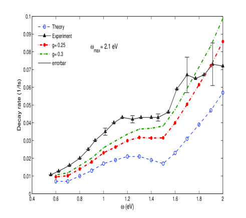
Figure 1: (Color online) Quasi particle decay rate in HOPG graphite. The triangles indicate TRPES measurements in Ref. moos , the open circles are ab-initio GW calculation of Ref. spataru . Filled circles and dashed lines show the total decay rate in presence of a new decay mechanism caused by triplet bosons for the electron-boson couplings $g=0.25,0.3$. In this calculation we have taken $\omega_{\rm max}=2.1$ eV. See the text for explanation.

As can be seen, a dispersive bosonic collective mode can account for the missing decay rate in HOPG graphite. The same result applies to undoped graphene as well. The fact that GW approximation falls a factor of two behind the experimentally measured decay rate, indicates that in addition to incoherent electron-hole decay processes, there should be another decay channel provided by a coherent bound state of electron-hole pairs, which is what our phenomenological Hamiltonian (1) describes. A simple RPA analysis showed that such a bound state can occur in triplet channel baskaranjafari ; jafaribaskaran .

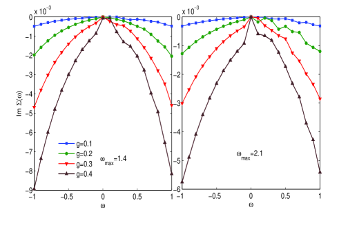
Figure 2: (Color online) Imaginary part of self-energy $vs$ energy (eV) for $\omega(q)_{max}=1.4eV$, $\omega(q)_{max}=2.1eV$.

III.2 Dependence on $\omega_{\rm max}$

The dispersion of triplet bosonic mode is over a wide energy range from zero to $\omega_{\rm max}\sim 2.1$ eV. The shape of dispersion and the value of $\omega_{\rm max}$ in the original work or Ref. baskaranjafari ; jafaribaskaran is essentially controlled by the short range part of the interaction (Hubbard $U$). It was also shown that the long-range part of the Coulomb interaction does not play a crucial role in the dispersion of the spin-1 collective mode jafaribaskaran . In the present calculation, we have fitted the dispersion relation obtained from the RPA analysis of Refs. baskaranjafari ; jafaribaskaran with $\sim 10$ cosine harmonics. over the whole Brillouin zone.

In Fig. 2 we explore the dependence of decay rates on the dispersion bandwidth ($\omega_{\rm max}$). Left panel shows the imaginary part of the self-energy for various values of the electron-boson coupling $g$, and for $\omega_{\rm max}=1.4$, while the left panel shows the same result for $\omega_{\rm max}=2.1$. As can be seen in both panels, by increasing the coupling strength $g$, the decay rate at a given energy scale increases. Comparison of the left and right panels for the same values of $g$ shows that smaller width of dispersion ($\omega_{\rm max}$), the bosonic mode leads to stronger spin flip scattering. The limit $\omega_{\rm max}\to 0$ can be thought of an Einstein like phonon mode which was studied within MA(1) in Ref berciu-graphene . Smaller $\omega_{\rm max}$ in our phenomenological Hamiltonian (1) corresponds to larger $U$ in the Hamiltonian of the original electrons in Ref. jafaribaskaran . Hence the observation of Fig. 2 can be justified as follows: In terms of the Hubbard type Hamiltonian of Ref. baskaranjafari , larger $U$ naturally leads to stronger decay rates.

III.3 Spectral function

Once we calculate the self-energy $\Sigma^{\alpha,\alpha}(\omega)$ at any approximation, we are able to immediately calculate the spectral weight $A(\vec{k},\omega)=-\frac{1}{2\pi}\mbox{Im}[\mbox{Tr}G_{\alpha,\alpha}(\vec{k},\omega)]$. We have plotted the spectral weight along high-symmetry cut $\Gamma-K-M$ of the Brillouin zone in Fig. 3. We have plotted the spectral weight for different energies. Panels (a)-(d) correspond to different values of $g$ as indicated in the figure caption.

The first point to notice in all panels is that the cone like dispersion of the Dirac electrons remains quite robust against increase in the electron-boson coupling $g$. To see this more transparently, in panel (a) we have plotted some negative energy spectral functions as well. As can be seen in panel (d), large values of coupling $g\sim 1$ lead to a remarkable broadening in the quasi particle peaks. Direct comparison with ARPES experiments on graphene indicates that $g$ can not be as large as $g\sim 1$.

Negative energy plots of panel (a) indicates that there is an asymmetry between the positive energy states and the negative energy states. This is natural, as the collective mode is an excitation and does not carry negative energies.

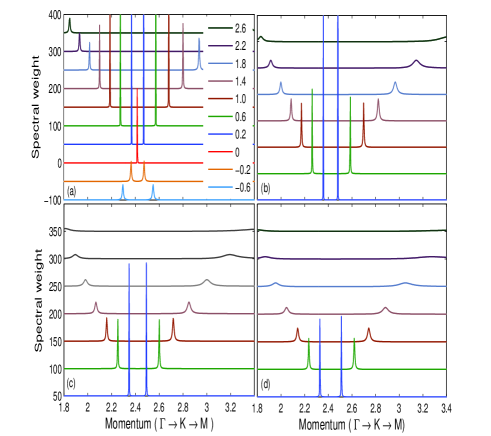
Figure 3: The spectral weight along high-symmetry cut in the $BZ$ for $\omega_{max}=2.1eV$ and (a) $g=0.3$ for different energy from -0.6 to 2.6 eV, (b) $g=0.6$, (c) $g=0.8$, (d) $g=1.0$ for different energy from 0.2 to 2.6 eV

IV conclusion

In this work we considered a phenomenological Hamiltonian containing a neutral spin-1 collective mode as a new bosonic branch of excitaitons predicted to exist in HOPG and undoped graphene baskaranjafari . Employing the momentum average self-energy we showed that such a coherent particle-hope bound state in triplet channel can account for substantial part of the missing decay rate in TRPES experiment of Ref. moos in HOPG. Another supporting evidence for existence of such a spin-1 collective mode which is a natural generalization of triplet excitations of ordinary semiconductors to the case of semi metallic HOPG comes from the downward renormalization of $v_{F}$ andrei . Apparently phonons fail to account for such renormalization. Moreover, the remarkable observation of Bose metal-insulator transition tuned by magnetic field in HOPG bosemetal , might indicate that there such spin excitation branch can have interesting consequences for the behavior of HOPG and graphene in magnetic fields.

V acknowledgement

We wish to thank M.R. Abolhassani, Y. Kopelevich, M. Berciu and G. Baskaran for comments and suggestions. S.A.J. was supported by the Vice Chancellor for Research Affairs of the Isfahan University of Technology, and the National Elite Foundation (NEF) of Iran.

Appendix A Generalization of MA(1) for spin-flip Hamiltonians

We start by writing Eqn. (4) with explicit spin indices. The matrix elements of Green’s function become,

$$G_{\uparrow,\uparrow}(\vec{k},\omega)= \!\!G_{0}(\vec{k},\omega)[1\!+\!g\!\sum_{\vec{k},\vec{q}_{1}}\!F^{\uparrow,\downarrow}_{1}(\vec{k},\vec{q}_{1},+1;\omega)]$$ (10)

$$G_{\downarrow,\downarrow}(\vec{k},\omega)= \!\!G_{0}(\vec{k},\omega)[1\!+\!g\!\sum_{\vec{k},\vec{q}_{1}}\!F^{\downarrow,\uparrow}_{1}(\vec{k},\vec{q}_{1},-1;\omega)]$$ (11)

$$G_{\uparrow,\downarrow}(k,\omega)= \!\!\!G_{0}(k,\omega)[g\sum_{k,q_{1}}F^{\uparrow,\uparrow}_{1}(k,q_{1},-1;\omega)]$$ (12)

$$G_{\downarrow,\uparrow}(\vec{k},\omega)= \!\!\!G_{0}(\vec{k},\omega)[g\sum_{\vec{k},\vec{q}_{1}}F^{\downarrow,\downarrow}_{1}(\vec{k},\vec{q}_{1},+1;\omega)].$$ (13)

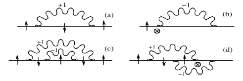
Figure 4: First and second order Feynman diagrams for the scattering vertex from a spin-1 collective mode. At each vertex the spin of electron is flipped. Therefore, the incoming and outgoing spins end up to be identical as in diagrams (a), (c). However, if we insist to have the spin of outgoing state to be opposite to that of incoming state, some vertices (denoted by $\otimes$) will not do flip the spin; that is they will not correspond to scattering from a spin-1 collective mode, as in diagrams (b), (d).

As can be intuitively seen in Fig 4, the non diagonal element of Green’s function should be zero. To see this more systematically, one writes the one bosons Green’s function as,

$$\sum_{\vec{k},\vec{q}_{1}}F^{\uparrow,\uparrow}_{1}(\vec{k},\vec{q}_{1},-1;\omega)=\frac{G_{\downarrow,\uparrow}(\vec{k},\omega)}{gG_{0}(\vec{k},\omega)}.$$ (14)

Repeating the equation of motion we obtain the two boson amplitude:

$$\sum_{\vec{q}_{1},\vec{q}_{2}}F^{\uparrow,\downarrow}_{2}(\vec{k},\vec{q}_{1},\vec{q}_{2},-1,+1;\omega)=$$ (15)

$$\frac{G_{\downarrow,\uparrow}(\vec{k},\omega)}{gG_{0}(\vec{k},\omega)}\left[\frac{1}{gG_{0}(\vec{k},\omega)}-gG_{0}(\vec{k}-\vec{q},\omega-\omega(\vec{q}))\right]$$

Finally for order $N+1$, we obtain for even $N$:

$$\sum_{\vec{k},\vec{q}_{1},\vec{q}_{2},...,\vec{q}_{N+1}}F^{\alpha,\alpha}_{N+1}(\vec{k},\vec{q}_{1},\vec{q}_{2},...,+1,-1,...;\omega)=$$

$$A(\vec{k},\vec{q}_{1},\vec{q}_{2},...,+1,-1,...;\omega)G_{\uparrow,\downarrow}(\vec{k},\omega)=0,$$ (16)

and for odd $N$:

$$\sum_{\vec{k},\vec{q}_{1},\vec{q}_{2},...,\vec{q}_{N+1}}F^{\uparrow,\downarrow}_{N+1}(\vec{k},\vec{q}_{1},\vec{q}_{2},...,+1,-1,...;\omega)=$$

$$B(\vec{k},\vec{q}_{1},\vec{q}_{2},...,+1,-1,...;\omega)G_{\uparrow,\downarrow}(\vec{k},\omega)=0.$$ (17)

The $A,B$ coefficients for various orders can be seen by inspection to be non zero. This proves that the spin off-diagonal components of the Green’s function are zero. This can be seen intuitively in Fig. 4.

To proceed further, we define a modified form of the bosonic Green’s function in MA(1) approximation as:

$$f^{\alpha,-\alpha}_{n}(\vec{k},\vec{q}_{1},...,\vec{q}_{n},...+1,-1,...;\omega)=$$

$$\frac{g^{n}F^{\alpha,(-1^{n})\alpha}_{n}(\vec{k},\vec{q}_{1},...,\vec{q}_{n},...+1,-1,...;\omega)}{G_{\alpha,\alpha}(\vec{k},\omega)}.$$ (18)

By inserting this in Eq.(4) one finds,

$$G_{\alpha,\alpha}(\vec{k},\omega)=$$

$$\!\!\!\!\!\!\!\!\!\!G_{0}(\vec{k},\omega)[1+g\sum_{\vec{k},\vec{q}_{1}}f^{\alpha,-\alpha}_{1}(\vec{k},\vec{q}_{1},1;\omega)G_{\alpha,\alpha}(\vec{k},\omega)].$$ (19)

where the matrix form of the Green’s function is:

$$G(k,\omega)=\left(\begin{array}[]{cc}G_{\uparrow,\uparrow}(\vec{k},\omega)&0\\ 0&G_{\downarrow,\downarrow}(k,\omega)\end{array}\right).$$ (22)

Dyson’s equation,

$$G_{\alpha,\alpha}(\vec{k},\omega)=[\omega-\epsilon_{\vec{k}}-\Sigma^{\alpha,\alpha}(\vec{k},\omega)+i\eta]^{-1},$$ (23)

give the spin diagonal self-energy as,

$$\Sigma^{\alpha,\alpha}(\omega)=\sum_{\vec{k},\vec{q}_{1}}f^{\alpha,-\alpha}_{1}(\vec{k},\vec{q}_{1},+1;\omega).$$ (24)

So the MA(1) self-energy is diagonal and can be casted into the final form given by Eq. (8), where

$$A_{1}(\omega) = \frac{\bar{g}_{0,2}(\omega)}{1-\frac{2\bar{g}_{0,3}(\omega)\bar{g}_{0,2}(\omega)}{1-\ldots}},$$

$$A_{2}(\omega) = \frac{2\bar{g}_{0,2}(\omega)}{1-\frac{3\bar{g}_{0,3}(\omega)\bar{g}_{0,2}(\omega)}{1-\ldots}},$$ (25)

$$\bar{g}_{0,n}(\omega) = \sum_{\vec{k},\vec{q}_{1},...,\vec{q}_{n}}G_{0}(\vec{k}-\sum_{i}\vec{q}_{i},\omega-\sum_{i}\omega_{\vec{q}_{i}}).$$

References

- (1) K. S. Novoselov, A. K. Geim, S. V. Morozov, D. Jiang, Y. Zhang, S. V. Dubonos, I. V. Grigorieva, and A. A. Firsov, Science 306, 666 (2004); K. S. Novoselov, A. K. Geim, S. V. Morozov, D. Jiang, M. I. Katsnelson, I. V. Grigorieva, S. V. Dubonos, A. A. Firsov, Nature 438, 197 (2005).
- (2) For a review see: A. H. Castro Neto, F. Guinea, N. M. R. Peres, K. S. Novoselov, A. K. Geim, Rev. Mod. Phys. 81, 109 (2009).
- (3) G. W. Semenoff, Phys. Rev. Lett. 53, 2449 (1984).
- (4) Xu Du, I. Skachko, A. Barker, E. Y. Anderi, Nature Nanotech. 3, 495 (2007).
- (5) R. Saito, Physical Properties of Carbon Nanotubes, World Scientific, 1998.
- (6) I. A. Luk’yanchuk, Y. Kopelevich, Phys. Rev. Lett. 93, 166402 (2004).
- (7) S. Y. Zhou, G.-H. Gweon, J. Graf, A. V. Fedorov, C. D. Spataru, R. D. Diehl, Y. Kopelevich, D.-H. Lee, S. G. Louie, A. Lanzara, Nature Phys. 2, 595-599 (2006).
- (8) G. Baskaran, S. A. Jafari, Phys. Rev. Lett. 89, 016402 (2002).
- (9) S. A. Jafari, G. Baskaran, Eur. Phys. J. B. 43, 175 (2005).
- (10) G. Moos, C. Gahl, R. Fasel, M. Wolf and T. Hertel, Phys. Rev. Lett. 87, 267402 (2001).
- (11) C. D. Spataru, M. A. Cazalilla, A. Rubio, L. X. Benedict, P. M. Echenique and S. G. Louie Phys. Rev. Lett. 87, 246405 (2001).
- (12) A. Bostwick, T. Ohta, T. Seyller, K. Horn, and E. Rotenberg. Nature Physics 3, 36 (2007).
- (13) E. H. Hwang, Ben Yu-Kuang Hu and S. Das Sarma, Phys. Rev. B. 76, 115434 (2007).
- (14) E. H. Hwang, S. Das Sarma, Phys. Rev. B. 75, 205418 (2007).
- (15) J. Gonzalez, F. Guinea and M. A. H. Vozmediano, Phys. Rev. Lett. 77, 3589 (1996); J. Gonzalez, F. Guinea and M. A. H. Vozmediano, Phys. Rev. B. 63, 134421 (2001).
- (16) J. Gonzalez, E. Perfetto, Phys. Rev. Lett. 101, 176802 (2008); Cheol-Hwan Park, F. Giustino, Marvin L. Cohen, S. G. Louie, Phys. Rev. Lett. 99, 086804 (2007).
- (17) G. Li, A. Luican and E. Y. Andrei. arXiv:0803.4016 (2008); J.L. McChesney, A. Bostwick, T. Ohta, K. Emtsev, T. Seyller, K. Horn, E. Rotenberg, arXiv:0809.4046 (2008).
- (18) Y. Kopelevich, Braz. J. Phys. 33, 737 (2003); Y. Kopelevich, J.C.Medina Pantoja, R. R. da Silva, S. Moehlecke, Phys. Rev. B 73, 165128 (2006).
- (19) M. Berciu, Phys. Rev. Lett. 97, 036402 (2006).
- (20) G. Baskaran, E. Tosatti, Current Science, 61, 33 (1991).
- (21) S. Pathak, V. B. Shenoy, G. Baskaran, arXiv:0809.0244v1
- (22) Glen L. Goodvin, Mona Berciu, and George A. Sawatzky, Phys. Rev. B. 74, 245104 (2006); M. Berciu and G. L. Goodvin, Phys. Rev. B 76, 165109 (2007).
- (23) L. Covaci and M. Berciu, Phys. Rev. Lett. 100, 256405 (2008).
- (24) G. D. Mahan, (Plenum, New York, 1981).