Decoherence-enhanced measurements

Quantum-enhanced measurements use highly non-classical quantum states in order to enhance the sensitivity of the measurement of classical quantities, like the length of an optical cavity Giovannetti04 . The major goal is to beat the standard quantum limit (SQL), i.e. a sensitivity of order $1/\sqrt{N}$, where $N$ is the number of quantum resources (e.g. the number of photons or atoms used), and to achieve a scaling $1/N$, known as the Heisenberg limit. Doing so would have tremendous impact in many areas Huelga97 ; Goda08 ; Budker07 , but so far very few experiments have demonstrated a slight improvement over the SQL Leibfried05 ; Nagata07 ; Higgins07 . The required quantum states are generally difficult to produce, and very prone to decoherence. Here we show that decoherence itself may be used as an extremely sensitive probe of system properties. This should allow for a new measurement principle with the potential to achieve the Heisenberg limit without the need to produce highly entangled states.

Decoherence arises when a quantum system interacts with an environment with many uncontrolled degrees of freedom, such as the modes of the electromagnetic field, phonons in a solid, or simply a measurement instrument Zurek91 . Decoherence destroys quantum mechanical interference, and plays an important role in the transition from quantum to classical mechanics Giulini96 . It becomes extremely fast if the “distance” between the components of a “Schrödinger cat”-type superposition of quantum states reaches mesoscopic or even macroscopic proportions. Universal power laws rule the scaling of the decoherence rates in this regime Braun01 and lead to time scales so small that in fact the founding fathers of quantum mechanics postulated an instantaneous collapse of the wave-function during measurement. Only recently could the collapse be time-resolved in experiments with relatively small “Schrödinger cat”–states Brune96 ; Guerlin07 . However, different superpositions may decohere with very different rates. In particular, if the coupling of the quantum system to the environment enjoys a certain symmetry, entire decoherence-free subspaces (DFS) may exist, in which superpositions of states retain their coherence, regardless of the “distance” between the superposed states. In essence, the symmetry prevents the environment to distinguish the states, such that no information leaks out of the system and the quantum superpositions remain intact. DFS have found widespread use in quantum information theory after their formulation for Markovian master equations Zanardi97 ; Lidar98 ; Duan98 , experimental demonstration Kwiat00 ; Kielpinski01 ; Viola01 , and once it was realized that quantum computation might be performed inside a DFS Beige00 . Given the reliance of the DFS on a symmetry in the coupling to the environment, it is clear that for a large “Schrödinger cat”-type superposition prepared in a DFS, the decoherence rate should be extremely sensitive to any changes that modify the symmetry of the coupling. This is the basic idea underlying the new measurement principle which we call “Decoherence-Enhanced Measurements” (DEM). Two fortunate circumstances make us believe that this idea may be turned into something of practical relevance. First, while it may seem that DEMs would again require the extremely difficult initial preparation of a highly entangled macroscopic state, surprisingly the Heisenberg limit can be reached with a much simpler to prepare product state of pairs of atoms. Second, the required initial “symmetry” of the coupling to the environment means nothing more but a degenerate eigenvalue of the Lindblad operators in the master equation, or, more generally, of the coupling Hamiltonian of the system to the environment Lidar98 . Actual symmetries in the system (e.g. spatial symmetries) may lead to such degeneracy, but are by no means necessary Braun01B . The scheme is therefore much more general than it may appear at first sight.

In order to illustrate the concept, we consider $N$ two–level atoms or ions ($N$ even, ground and excited states $|0\rangle_{i}$, $|1\rangle_{i}$ for atom $i$, $i=1,\ldots,N$) localized in a cavity with one semi-reflecting mirror, and resonantly coupled with coupling constants $g_{i}$ to a single e.m. mode of the cavity of frequency $\omega$. The reduced density matrix $\rho$ of the atoms evolves according to the master equation in the interaction picture

$$\frac{d}{dt}\rho(t)={\cal L}_{s}[\rho(t)]+{\cal L}_{c}[\rho(t)]\,,$$ (1)

where

$${\cal L}_{s}[\rho(t)]=\frac{\Gamma}{2}\sum_{i=1}^{N}\left(\big{[}\sigma_{-}^{(i)}\rho(t),\sigma_{+}^{(i)}\big{]}+\big{[}\sigma_{-}^{(i)},\rho(t)\sigma_{+}^{(i)}\big{]}\right)$$ (2)

describes individual spontaneous emission with rate $\Gamma$, while

$${\cal L}_{c}[\rho(t)]=\gamma\,([J_{-}\rho(t),J_{+}]+[J_{-},\rho(t)J_{+}])$$ (3)

models collective decoherence, $J_{-}=\sum_{i=1}^{N}\tilde{g}_{i}\sigma_{-}^{(i)}$, $J_{+}=J_{-}^{\dagger}$, $\sigma^{(i)}_{+}=|1\rangle_{i}\langle 0|_{i}$ ($\sigma^{(i)}_{-}=|0\rangle_{i}\langle 1|_{i}$), and $\tilde{g}_{i}=g_{i}/g$ where $g$ is the average coupling strength over all atoms coupled to the cavity field. The rate $\gamma=g^{2}/\kappa$ (with $\kappa$ the single photon cavity decay rate) is independent of $N$. Equation (1) is a well–known and experimentally verified Gross76 ; Skribanowitz73 master equation which for $\tilde{g}_{i}=1\,\,\forall i$ and in the bad cavity limit $\Gamma\ll g\sqrt{N}\ll\kappa$ describes superradiance Agarwal70 ; Bonifacio71a ; Glauber76 ; Gross82 . Due to the spatial envelope of the e.m. mode in resonance with the atoms, the $g_{i}$ depend on the position $x_{i}$ of the atoms along the cavity axis and on the length $L$ of the cavity (the waist of the mode is taken to be much larger than the size of the atomic ensemble),

$$g_{i}=\sqrt{\frac{\hbar\omega}{\epsilon_{0}V}}\sin(k_{x}x_{i})\,\mbox{\boldmath{$\epsilon$}}\cdot{\bf d}\,,$$ (4)

where $k_{x}=\pi n_{x}/L$, $\epsilon_{0}$ denotes the dielectric constant of vacuum, $V=LA$ the mode volume (with an effective cross–section $A$), $\epsilon$ the polarization vector of the mode, and ${\bf d}$ the vector of electric dipole transition matrix elements between the states $|0\rangle_{i}$ and $|1\rangle_{i}$, taken identical for all atoms. Decoherence in this system has been extensively studied, see Braun01B for a review. The initial state $\rho_{0}=|\psi_{0}\rangle\langle\psi_{0}|$ belongs to the DFS with respect to collective emission, ${\cal L}_{c}[\rho_{0}]=0$, if and only if $J_{-}|\psi_{0}\rangle=0$ Lidar98 . If $\tilde{g}_{i}=1$ for $i=1,\ldots,N$, this DFS is well known Beige00b ; Braun01B . It contains ${N\choose N/2}\sim 2^{N}/\sqrt{N}$ DF states, including a $2^{N/2}$ dimensional subspace $\bigotimes_{l=1}^{N/2}\{|t_{-}\rangle_{l},|s\rangle_{l}\}$ in which the pair formed by the atoms $l$ and $l+N/2$ can be in a superposition of the triplet ground state $|t_{-}\rangle_{l}=|0\rangle_{l}|0\rangle_{l+N/2}$ and the singlet $|s\rangle_{l}=\frac{1}{\sqrt{2}}(|0\rangle_{l}|1\rangle_{l+N/2}-|1\rangle_{l}|0\rangle_{l+N/2})$. For arbitrary $\tilde{g}_{i}$, $|s\rangle_{l}$ should be replaced by $\frac{1}{\sqrt{|\tilde{g}_{l}|^{2}+|\tilde{g}_{l+N/2}|^{2}}}(\tilde{g}_{l}|0\rangle_{l}|1\rangle_{l+N/2}-\tilde{g}_{l+N/2}|1\rangle_{l}|0\rangle_{l+N/2})$.

Consider now the situation where the atoms can be grouped into two sets with $N/2$ atoms each and coupling constants $G_{1}$ in the first set ($i\in S_{1}\equiv\{1\ldots,N/2\}$), and $G_{2}$ in the second set ($i\in S_{2}\equiv\{N/2+1,\ldots,N\}$). One way of obtaining two coupling constants may be to trap the atoms in two two–dimensional lattices perpendicular to the cavity axis (see Fig.1).

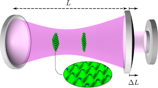
Figure 1: $N$ atoms (or ions) are trapped at fixed positions in two 2D optical lattices perpendicular to the cavity axis. A dipole transition of the atoms is in resonance with a single, leaky cavity mode. The atoms are initially prepared in a DFS state relative to a given cavity length. When the cavity length changes slightly, the DFS evolves, and the initial state is exposed to collective decoherence, detectable by photons leaking out through the semi-reflecting mirror at a rate proportional to $N^{2}$.

Suppose that after preparing the atoms in a DFS state corresponding to the initial couplings $\tilde{G}_{I}^{(0)}=G_{I}^{(0)}/g$ ($I=1,2$), the length $L$ of the cavity changes slightly. The coupling constants will evolve, $\tilde{G}_{I}^{(0)}\rightarrow\tilde{G}_{I}\equiv G_{I}/g$, and so will the DFS. It is this collective change of the coupling constants which can be revealed very sensitively through the decoherence it induces as the original state becomes exposed to decoherence. The induced decoherence therefore provides for a very precise measurement of the change of the length of the cavity, as we shall show now.

In order to simplify notation we will assume in the following $\tilde{G}_{1}^{(0)}=\tilde{G}_{2}^{(0)}$ (i.e. the atoms are located for instance symmetrically with respect to an antinode of the cavity mode, or at a distance given by an integer multiple of the wavelength of the mode), but we emphasize that everything goes through for different initial couplings, unless otherwise mentioned. Assume that an initial pure product state of pairs of atoms is prepared in the initial DFS, $\rho_{0}=|\psi_{0}\rangle\langle\psi_{0}|$, where

$$|\psi_{0}\rangle=\bigotimes_{l=1}^{N/2}|\varphi_{l}\rangle_{l}$$ (5)

with $|\varphi_{l}\rangle_{l}=a_{l}|t_{-}\rangle_{l}+b_{l}|s\rangle_{l}$. The decoherence mechanism (3) is directly linked to photon loss from the cavity. The induced decoherence can be measured through the number of photons $n_{\rm ph}$ which escape through the cavity mirror during a small time interval $\Delta t$. In the superradiant regime considered here ($\Gamma\ll g\sqrt{N}\ll\kappa$), any photon created leaves the cavity immediately, such that the quantum expectation value of $n_{\rm ph}$ is given by $\langle n_{\rm ph}\rangle=-\langle\dot{J}_{z}(t=0)\rangle_{c}\Delta t=-{\rm tr}\big{(}J_{z}\mathcal{L}_{c}[\rho_{0}]\big{)}\Delta t$, where the collective pseudo-spin component $J_{z}=\frac{1}{2}\sum_{i=1}^{N}\sigma_{z}^{(i)}$ measures total population inversion of the atoms. As long as $|\psi_{0}\rangle$ resides in the DFS, we have $\langle n_{\rm ph}\rangle=0$. If the coupling constants undergo slight changes and get replaced by general values $\tilde{g}_{i}$ for atom $i$, a straightforward calculation (see Methods) shows that

$$\langle\dot{J}_{z}(0)\rangle_{c} = -\gamma\Big{(}\sum_{i=1}^{N/2}|\tilde{g}_{i}-\tilde{g}_{i+N/2}|^{2}|b_{i}|^{2}$$ (6)

$$+\sum_{\stackrel{{\scriptstyle i,j=1}}{{i\neq j}}}^{N/2}\left(\tilde{g}_{i}^{*}-\tilde{g}_{i+N/2}^{*}\right)\left(\tilde{g}_{j}-\tilde{g}_{j+N/2}\right)b_{i}^{*}b_{j}a_{i}a_{j}^{*}\Big{)}\,,$$

which is in general of order $N^{2}$. In particular, if the $\tilde{G}_{I}$ undergo collective changes $\tilde{G}_{I}^{(0)}\rightarrow\tilde{G}_{I}$ with $\tilde{G}_{1}\neq\tilde{G}_{2}$ and if all pairs of atoms were prepared in the same initial state $a_{l}=a$, $b_{l}=b$ for $l=1,2,\ldots,N/2$, we have

$$\langle\dot{J}_{z}(0)\rangle_{c} = -\gamma|\delta\tilde{G}|^{2}f(N,b)$$ (7)

$$f(N,b) = 4|b|^{2}\Big{[}\frac{N}{2}+\frac{N}{2}\left(\frac{N}{2}-1\right)(1-|b|^{2})\Big{]}\,\,,$$ (8)

where $\delta\tilde{G}\equiv(\tilde{G}_{1}-\tilde{G}_{2})/2$. The term quadratic in $N$ is maximized for $|b|=1/\sqrt{2}$, i.e. an equal weight superposition of the two DF basis states $|t_{-}\rangle_{l}$ and $|s\rangle_{l}$ for each pair of atoms, and gives for $N\gg 1$ a signal $\langle n_{\rm ph}\rangle\simeq\gamma\Delta t|\delta\tilde{G}|^{2}N^{2}/4$. As long as the two lattices are not situated at anti-nodes of the mode, the relation between $\delta\tilde{G}$ and $\delta L/L$ is linear to lowest order. If we choose $x_{2}-x_{1}=m\lambda$ with $n_{x}-1\geq m\in\mathbb{N}$ we have

$$\delta\tilde{G}=m\pi\cot(\frac{n_{x}\pi x_{1}}{L})\frac{\delta L}{L}\,,$$ (9)

where we see that $\delta\tilde{G}$ and $\delta L/L$ are related by a factor independent of $N$. Note that the measurement of $\langle n_{\rm ph}\rangle$ allows the measurement of $\delta L/L$, and not just a detection of a change of $L$ : $\delta L/L=\Big{(}\langle n_{\rm ph}\rangle/(\gamma\Delta t(m\pi\cot(n_{x}\pi x_{1}/L))^{2}f(N,b))\Big{)}^{1/2}$. The ultimate sensitivity achievable depends not only on the scaling of the signal $\langle n_{\rm ph}\rangle$ with $N$, but also of the noise, quantified through the standard deviation $\sigma(n_{\rm ph})=(\langle n_{\rm ph}^{2}\rangle-\langle n_{\rm ph}\rangle^{2})^{1/2}$. The most fundamental noise associated with the measurement of $n_{\rm ph}$ is its fluctuation due to the quantum mechanical nature of the prepared state. Our approach of calculating initial time-derivatives of observables by tracing them over with the Lindbladian implies $\langle n_{\rm ph}\rangle\ll 1$, as $J_{-}$ can change the number of excitations by at most 1, and this condition sets an upper bound on $\Delta t$. In this regime, $\langle n_{\rm ph}^{2}\rangle\simeq\langle n_{\rm ph}\rangle$, and, therefore, $\sigma(n_{\rm ph})\simeq\sqrt{\langle n_{\rm ph}\rangle}$. It follows that the signal-to-noise ratio is given by $\langle n_{\rm ph}\rangle/\sigma(n_{\rm ph})\simeq|\delta\tilde{G}|\sqrt{\gamma\Delta t}\sqrt{f(N,b)}$. The ultimate sensitivity achievable can be estimated from a fixed $\langle n_{\rm ph}\rangle/\sigma(n_{\rm ph})$ of order 1, independent of $N$, which leads to a minimal $|\delta\tilde{G}|={\cal O}(1/(\sqrt{\gamma\Delta t}N))$. We have thus shown that a precision measurement based on the purely dissipative dynamics (3) and an initial product state can achieve the Heisenberg limit. This is in contrast to unitary dynamics of $N$ independent quantum resources, where the SQL cannot be surpassed when using an initial product state Giovannetti06 .

In a real experiment there may be additional fundamental noise sources. One obvious concern is spontaneous emission. It is easily verified that ${\cal L}_{s}[\rho_{0}]$ leads to a contribution $\langle\dot{J}_{z}(0)\rangle_{s}=-\Gamma\sum_{i=1}^{N/2}|b_{i}|^{2}$ to $\langle\dot{J}_{z}(0)\rangle$ which scales as ${\cal O}(N)$ and leads to a background signal against which, one might think, the collective decoherence signal $\langle\dot{J}_{z}(0)\rangle_{c}$ has to be compared. However, note that spontaneous emission sends photons into the entire open space but not into the cavity, whereas the collective emission escapes exclusively through the leaky cavity mirror. Therefore, the two contributions can be well separated by observing only the photons escaping through the cavity mirror.

Another obvious concern are fluctuations of the coupling constants. In order to measure $\langle n_{\rm ph}\rangle$, the experiment has to be repeated $\nu$ times with $\nu\gg 1$. However, $\nu$ is independent of $N$ and only given by the desired signal/noise, or, equivalently, by $\langle n_{\rm ph}\rangle$ itself. Increasing $\nu$ does therefore not influence the scaling with $N$. It increases the sensitivity by a factor $\sqrt{\nu}$, but reduces the bandwidth by $1/\nu$ in the standard way. While we assume that the time scale of the mirror motion is sufficiently long compared to the time needed for averaging, the exact coupling constants might fluctuate about their slowly evolving mean values during the averaging, e.g. due to fluctuating traps caused by vibrations in the set up. But even for perfectly stable traps, the micro–motion of the atoms in their respective trapping potentials, thermal motion, or even quantum fluctuations in the traps will lead to fluctuating $g_{i}$. The cost in sensitivity of these fluctuations depends on their correlations. To see this, let us consider fluctuations $\delta\tilde{g}_{i}$ of the $\tilde{g}_{i}$ about their mean values $\tilde{G}_{I}$, $\tilde{g}_{i}=\tilde{G}_{1}+\delta\tilde{g}_{i}$ for $i=1,\ldots,N/2$, $\tilde{g}_{i}=\tilde{G}_{2}+\delta\tilde{g}_{i}$ for $i=N/2+1,\ldots,N$. We introduce the correlation matrix $C_{ij}=\overline{\delta\tilde{g}_{i}^{*}\delta\tilde{g}_{j}}$, where the over-line denotes an average over the ensemble describing the fluctuations. Equation (6) then leads to a background $\alpha_{\rm bg}$ in the photon counting rate and to fluctuations $\delta\alpha_{f}$ on top of $\alpha_{c}\equiv-\langle\dot{J}_{z}(0)\rangle_{c}$, i.e. $\alpha=\alpha_{c}+\alpha_{\rm bg}+\delta\alpha_{f}$. The average background $\overline{\alpha}_{\rm bg}$, given by

$$\overline{\alpha}_{\rm bg} = \gamma\Big{\{}\sum_{i=1}^{N/2}\Big{(}C_{ii}+C_{i+\frac{N}{2}\,i+\frac{N}{2}}-C_{i\,i+\frac{N}{2}}-C_{i+\frac{N}{2}\,i}\Big{)}|b_{i}|^{2}\Big{\}}\,,$$

can be determined independently at $\delta\tilde{G}=0$, and subtracted from the signal; it does therefore not influence the sensitivity of the measurement. The remaining noise $\delta\alpha_{f}$ fluctuates about zero,

$$\delta\alpha_{f} = 2\gamma\Big{\{}\sum_{i=1}^{N/2}(\delta\tilde{G}^{*}\Delta\tilde{g}_{i}+\delta\tilde{G}\Delta\tilde{g}_{i}^{*})|b_{i}|^{2}+\sum_{\stackrel{{\scriptstyle i,j=1}}{{i\neq j}}}^{N/2}(\delta\tilde{G}^{*}\Delta\tilde{g}_{j}+\delta\tilde{G}\Delta\tilde{g}_{i}^{*})b_{i}^{*}b_{j}a_{i}a_{j}^{*}\Big{\}}\,,$$ (10)

where $\Delta\tilde{g}_{i}\equiv\delta\tilde{g}_{i}-\delta\tilde{g}_{i+N/2}$. Assuming real coupling constants, we find the standard deviation $(\overline{\delta\alpha_{f}^{2}})^{1/2}=4\gamma|\delta\tilde{G}|K$, where $K=(\sum_{i,j=1}^{N/2}(C_{i,j}+C_{i+N/2,j+N/2}-C_{i,j+N/2}-C_{i+N/2,j})S_{i}S_{j})^{1/2}$, and $S_{i}=|b_{i}|^{2}+b_{i}^{*}a_{i}\sum_{j|j\neq i}b_{j}a_{j}^{*}$ is in general of order ${\cal O}(N)$. This leads to fluctuations in the measured photon number with a standard deviation $(\overline{\delta n_{\rm ph}^{2}})^{1/2}$, and to a signal-to-noise ratio $\langle n_{\rm ph}\rangle/(\overline{\delta n_{\rm ph}^{2}})^{1/2}=|\delta\tilde{G}|f(N,b)/(4K)$.

Several interesting cases can be considered:

1. Fully uncorrelated fluctuations, $C_{ij}=C_{i}\delta_{ij}$, where $\delta_{ij}$ stands for the Kronecker-delta: Here we get $K=\left(\sum_{i=1}^{N/2}(C_{i}+C_{i+N/2})S_{i}^{2}\right)^{1/2}$, which is in general of order $N^{3/2}$, and leads back to the SQL.

2. Pairwise identical fluctuations between the two sets: $C_{ij}=C_{i+\frac{N}{2}\,j}=C_{i\,j+\frac{N}{2}}=C_{i+\frac{N}{2}\,j+\frac{N}{2}}$ for $i,j=1,\ldots,N/2$. This can be the consequence of fully correlated fluctucations, $C_{ij}=C\,\,\,\forall\,\,\,i,j$. Alternatively, such a situation arises for example for atoms initially arranged symmetrically with respect to an anti-node such that $\tilde{G}_{1}^{(0)}=\tilde{G}_{2}^{(0)}$, if the two atoms (or ions) in each pair $l$ ($l=1,\ldots,N/2$) are locked into a common oscillation. This should be the case for two trapped ions repelling each other through a strong Coulomb interaction, and cooled below the temperature corresponding to the frequency of the breathing mode. Equation (10) then gives $\delta\alpha_{f}=0$. Note, however, that for initial $\tilde{G}_{1}^{(0)}\neq\tilde{G}_{2}^{(0)}$ the more general DFS leads to a more complicated condition for the correlations, $C_{ij}|\tilde{G}_{2}^{(0)}|^{2}+C_{i+\frac{N}{2}\,j+\frac{N}{2}}|\tilde{G}_{1}^{(0)}|^{2}-C_{i\,j+\frac{N}{2}}\tilde{G}_{2}^{(0)*}\tilde{G}_{1}^{(0)}-C_{i+\frac{N}{2}\,j}\tilde{G}_{1}^{(0)*}\tilde{G}_{2}^{(0)}=0$, which might be harder to achieve.

3. Correlated fluctuations within a set, but uncorrelated between the two sets, $C_{ij}=C$ for $i,j\in S_{1}$ or $i,j\in S_{2}$, but $C_{ij}=0$ for $i\in S_{1}$ and $j\in S_{2}$ or vice versa. In this case both sums in (10) survive and lead to a noise of order ${\cal O}(N^{2})$, the worst case scenario. However, this comes to no surprise, as such correlations are indistinguishable from the signal: all the atoms in a given set move in a correlated fashion, but independently from the atoms of the other set. This leads to a collective difference in the couplings, just as if the length of the cavity was changed.

Case (2) above is clearly the most favorable situation. If there are no other background signals depending on $N$, we keep the $1/N$ scaling of $\delta\tilde{G}$ characteristic of the Heisenberg limit. In order to favor case (2) over cases (1),(3), it appears to be advantageous to work with ions and to try to bring the ions in a pair as closely together as possible, thus strongly correlating their fluctuations, while separating the ions in the same set as far as possible.

To summarize, we have shown for a particular example how the very sensitive dependence of collective decoherence on system parameters can be exploited to reach the Heisenberg limit in precision measurements while using an initial product state — something which is known to be impossible with unitary dynamics Giovannetti06 . It should be clear that the principle of DEM is far more general than the example exposed here. Decoherence is itself a process in which interference effects play an important role. This is exemplified by the very existence of DFS, and can lead to exquisite sensitivity. One might therefore as well try to exploit these effects instead of trying to suppress decoherence at all costs.

Methods
Derivation of Eq. (6): The commutation relation $[J_{\pm},J_{z}]=\mp J_{\pm}$, valid for any choice of couplings $\tilde{g}_{i}$, allows to rewrite $\langle\dot{J}_{z}(0)\rangle_{c}=-2\gamma\langle\psi_{0}|J_{+}J_{-}|\psi_{0}\rangle$. A short calculation yields $J_{-}|\psi_{0}\rangle=-(1/\sqrt{2})\sum_{i=1}^{N/2}(\tilde{g}_{i}-\tilde{g}_{i+\frac{N}{2}})b_{i}|t_{-}\rangle_{i}\bigotimes_{l\neq i}^{N/2}|\varphi_{l}\rangle_{l}$ and leads immediately to Eq. (6). Preparation of initial state: In order to prepare the product state (5) it is helpful to use three–level atoms with a lambda structure. Let $|0\rangle$ and the additional state $|2\rangle$ be hyperfine (HF) states, and assume that their energies are split in a sufficiently strong magnetic field, such that only the transition $|0\rangle\leftrightarrow|1\rangle$ resonates with the cavity mode. We assume further that the second optical lattice can be moved along the cavity axis, such that controlled pairwise collisions of corresponding atoms in the two lattices can be induced. Entangled pairs of atoms in their HF split ground states can thus be created (for atoms in the same lattice this has been demonstrated experimentally, see Bloch08 for a review). After the creation of an entangled HF state $|\psi^{\prime}_{0}\rangle$, that differs from (5) by the replacement of states $|1\rangle$ by states $|2\rangle$, the second lattice is moved back to its original position. Now one can selectively excite the $|2\rangle$ states by a laser pulse in resonance with the $|2\rangle\leftrightarrow|1\rangle$ transition, that replaces the singlets in the (very long lived) HF states by the desired singlets of the $|0\rangle$ and $|1\rangle$ states and thus produce the product state (5). However, as such, the method is not of much practical use yet, as it will be virtually impossible to park the second lattice at the exact position corresponding to coupling constants which render the state (5) decoherence free. The extreme sensitivity of the collective decoherence with respect to changes of the coupling constants plays against us here, and will lead to a superradiant flash of light from the cavity after the excitation $|\psi^{\prime}_{0}\rangle\to|\psi_{0}\rangle$, if the exact position corresponding to $|\psi_{0}\rangle\in$ DFS is not achieved. But it is possible to position the second lattice at the required position with a precision of ${\cal O}(1/N)$ for the case (2) considered above, using a feed-back mechanism and a part of the quantum ressources. With the atoms in the state $|\psi^{\prime}_{0}\rangle$, do the following repeatedly in order to find the optimal position: Excite a part of the entangled HF pairs containing ${\cal O}(N/\ln N)$ atoms with the laser, measure $\langle n_{\rm ph}\rangle$, and use the measurement results to bracket the minimum of $\langle n_{\rm ph}\rangle$ as function of the lattice position. The minimum of $\langle n_{\rm ph}\rangle$ indicates that the position corresponding to the DFS is achieved. Using golden section search, the minimum can be bracketed to precision $1/N$ in ${\cal O}(\ln N)$ moves, as at each step the sensitivity of the measurement of the position of the lattice is of order ${\cal O}(\ln N/N)\sim{\cal O}(1/N)$. Once the minimum is found, excite the remaining unused pairs (there should be still a number of pairs of ${\cal O}(N)$) to the desired state $|\psi_{0}\rangle$. That state is now decoherence-free, and the system ready to detect small changes of the position of one of the mirrors. Note that for this method it is not necessary to know which exact state is produced in the controlled collisions and subsequent laser excitation.

Imperfections in preparation of $|\psi_{0}\rangle$: Suppose that instead of the state (5) a state

$$|\tilde{\psi}_{0}\rangle=\bigotimes_{l=1}^{N/2}|\varphi\rangle_{l}\mbox{ with }|\varphi\rangle_{l}=a|t_{-}\rangle_{l}+b|s\rangle_{l}+c|t_{0}\rangle_{l}+d|t_{+}\rangle_{l}$$ (11)

was prepared (we consider the same state for all pairs for simplicity, but this is not essential). Repeating the calculation that leads to Eq. (8) and assuming real $\tilde{G}_{i}$, we now find

$$\langle n_{\rm ph}\rangle = \gamma\Delta t\Big{[}\frac{N}{2}\Big{(}\big{(}(c-b)\tilde{G}_{1}+(c+b)\tilde{G}_{2}\big{)}^{2}+d^{2}(\tilde{G}_{1}^{2}+\tilde{G}_{2}^{2})\Big{)}$$ (12)

$$+\frac{N}{2}\left(\frac{N}{2}-1\right)\Big{(}(\tilde{G}_{2}-\tilde{G}_{1})b(a-d)+(\tilde{G}_{2}+\tilde{G}_{1})c(a+d)\Big{)}^{2}\Big{]}\,.$$

The derivative of $\langle n_{\rm ph}\rangle$ with respect to $\tilde{G}_{2}$ is of order ${\cal O}(N^{2})$, and thus still allows to find the minimum of $\alpha$ as function of the position of the second lattice with a precision of order ${\cal O}(1/N)$ in case 2. At the minimum a component outside the DFS persists, such that photons will leak out of the cavity, but the average background is only of order ${\cal O}(N)$, and can be measured separately and subtracted from the singal. Changes $\delta\tilde{G}_{2}$ of $\tilde{G}_{2}$ away from the position of the minimum still lead to a signal that scales, for large $N$, quadratically with $N$, $\langle n_{\rm ph}\rangle=\frac{\gamma\Delta t}{4}\left(a(c+b)+d(c-b)\right)^{2}N^{2}\delta\tilde{G}_{2}^{2}$, and the previous analysis leading to the Heisenberg limit still applies.

Alternatively, one can get rid of the additional background by letting the system relax before measuring changes of $L$. Indeed, any state with a component outside the DFS will relax to a DFS state (and thus a dark state) or mixtures of DFS states within a time of order $1/\gamma$ or less. Components with large total pseudo-angular momentum $J$ relax in fact in much shorter time of order $1/(J\gamma)$. The DFS states reached through relaxation starting from $|\tilde{\psi}_{0}\rangle$ still allow a scaling of $\langle n_{\rm ph}\rangle$ close to $N^{2}$. We have shown this by simulating the relaxation process with the help of the stochastic Schrödinger equation (SSE) corresponding to Eq. (3). For real values of the coupling constants, the SSE reads

$$d\psi(t) = D_{1}(\psi(t))\,dt+D_{2}(\psi(t))\,dW(t)$$ (13)

$$D_{1}(\psi) = \gamma\left(2\langle J_{-}\rangle_{\psi}J_{-}-J_{+}J_{-}-\langle J_{-}\rangle^{2}_{\psi}\right)\psi$$ (14)

$$D_{2}(\psi) = \sqrt{2\gamma}\left(J_{-}-\langle J_{-}\rangle_{\psi}\right)\psi\,,$$ (15)

where $dW(t)$ is a Wiener process with average zero and variance $dt$, and $\langle J_{-}\rangle_{\psi}=\langle\psi|J_{-}|\psi\rangle$ Breuer06 . Using an Euler scheme with a time step of $0.01/\gamma$, we followed the convergence of $\psi(t)$ to DFS states for states with $(a,b,c,d)=(\cos\delta,1,0,\sin\delta)/\sqrt{2}$, until the norm of the difference $|\psi(t+dt)\rangle-|\psi(t)\rangle$ dropped below $10^{-12}$. In these final dark states, randomly distributed over the DFS, we calculated $\alpha$, and averaged over a large number $n_{r}$ of realizations of the stochastic process ($n_{r}=10^{5}$, $10^{4}$, $10^{4}$, $2.5\cdot 10^{3}$, $10^{3}$, $1.25\cdot 10^{3}$, 250, 200, and 250 for $N=2,4,6,8,10,12,14,16$, and $18$). Figure 2 shows the scaling of $\alpha$ as function of $N$ for different values of $\delta$ for $0\leq\delta\leq\pi/2$ up to $N=18$. Within this numerically accessible range of $N$, $\alpha$ follows a power law $\alpha\propto N^{p}$ with an exponent $p$ that decays only gradually with $\delta$ for $\delta\leq\pi/4$. Moreover, that decay might be a finite size effect: Note that, surprisingly, $\alpha(\delta)$ appears to be close to symmetric with respect to $\delta=\pi/4$. This is corroborated by exact analytical calculations based on the diagonalization of ${\cal L}_{c}$, which lead to $\alpha=1/2$ for $N=2$, $\alpha=(55-12\sin(2\delta)-\cos(4\delta))/36$ for $N=4$, and $\alpha=(303-110\sin(2\delta)-3\cos(4\delta))/100$ for $N=6$ (in units $\gamma|\tilde{G}_{1}-\tilde{G}_{2}|^{2}$). The plot shows that all numerical data can be very well fitted by $\alpha=A+B\sin(2\delta)+C\cos(4\delta)$. From Eq. (8) we know that $A+C$ has to scale as $N^{2}$ for sufficiently large $N$. Both $B$ and $C$ are negative for all $N$ for which we have data, and $C$ appears to be negligible. Fig. 2 shows that $-B$ increases even more rapidly than $N^{2}$ (a fit in the range $N=8,\ldots,18$ gives a power law $N^{2.4}$). But $B$ has to cross over to a power law $N^{p}$ with $p\leq 2$, unless other Fourier components start contributing significantly. Otherwise, $\alpha$ would become negative for $\delta>0$. This indicates that for large $N$ the scaling of $\alpha$ is in fact $N^{2}$ for all $\delta$.

In summary, our method still works, even if the product state (5) is not prepared perfectly. One has the choice to start measurement immediately after state preparation, which gives an additional background of order $N$, or to wait a time of the order of a few $1/\gamma$ after preparation of the initial state, until no more photons leave the cavity through the mirror, with no additional background. In both cases the scaling of the signal-to-noise ratio is still $\sim\sqrt{\gamma\Delta t}|\delta L/L|N$, and allows to reach the Heisenberg limit in the measurement of a subsequent small change of $L$.

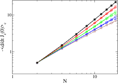
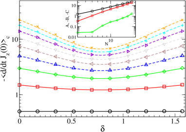
Figure 2: (a) Scaling of collective photon emission rate $\alpha=-\langle\dot{J}_{z}(0)\rangle_{c}$ (in units $\gamma|\tilde{G}_{1}-\tilde{G}_{2}|^{2}$) in the mixture of DFS states reached by relaxation from state $|\tilde{\psi}_{0}\rangle$, Eq. (11). Data for $\delta=\delta_{0}$ ($\delta=\pi/2-\delta_{0}$) denoted by squares and full lines (diamonds and dashed lines), respectively; $\delta_{0}=0,\pi/9,2\pi/9,3\pi/9$ and $4\pi/9$ in black, red, green, blue, and brown. Exact analytical results for $\delta=0$, Eq. (8) shown with black crosses. Full and dashed lines are guides to the eye only. (b) Dependence of $\alpha$ on $\delta$. $N=2$, 4,6,8,10,12,14,16,18 in black circles, red squares, green diamonds, blue triangles up, brown triangles left, grey triangles down, violet triangles right, cyan pluses, orange Xs, respectively. The full lines for $N$=2,4,6 are exact analytical results. The dashed lines for $N=8,\ldots,18$ are fits to $A+B\sin(2\delta)+C\cos(4\delta)$. The inset shows the scaling of the coefficients $A$ (black circles), $-B$ (red squares), and $-C$ (green diamonds) as function of $N$.

Another class of states in the DFS that allows quadratic scaling of $\alpha$ with $N$, are Schrödinger cat states of macroscopic pseudo-angular momentum $j_{1}=j_{2}\equiv\ell\sim N$ in the two sublattices (i.e. states $|(\ell,\ell)j,-j\rangle$),

$$\langle(\ell,\ell)j,-j|J_{1+}J_{1-}|(\ell,\ell)j,-j\rangle={} |\tilde{G}_{1}|^{2}\frac{(2j+1)(2j+2)}{4(j+1)^{2}-1}\left[\ell(\ell+1)-\frac{j(j+2)}{4}\right]\,,$$ (16)

with $J_{1-}=\tilde{G}_{1}\sum_{i=1}^{N/2}\sigma^{(i)}_{-}$ in agreement with the initial intuitive reasoning. If the total system is initially in a singlet state ($j=0$) and the angular momentum of each of the two sets of $N/2$ atoms has its maximal value $\ell=N/4$, we have

$$\langle n_{\rm ph}\rangle=\frac{\gamma\Delta t}{3}|\delta\tilde{G}|^{2}\,N(N+4)\,.$$ (17)

While these states are protected by the DFS and thus do not suffer the fate of rapid decoherence of the highly entangled states proposed for QEM, it appears to be still more challenging to produce them compared to the product states (5). Our numerical simulations also show that states chosen randomly inside the DFS lead on the average only to $\langle n_{\rm ph}\rangle\propto N$. Therefore, it is rather remarkable that the product states (5) and the above Schrödinger cat states share the property of scaling of $\langle n_{\rm ph}\rangle\propto N^{2}$.

The authors declare to have no competing financial interests.

Acknowledgments: DB thanks Eite Tiesinga and Peter Braun for useful discussions. This work was supported by the Agence National de la Recherche (ANR), project INFOSYSQQ. Numerical calculations were partly performed at CALMIP, Toulouse. J.M. thanks the Belgian F.R.S.-FNRS for financial support.

References

- (1) Giovannetti, V., Loyd, S., & Maccone, L., Quantum-Enhanced Measurements: Beating the Standard Quantum Limit, Science 306, 1330 (2004).
- (2) Huelga, S. F. et al., Improvement of Frequency Standards with Quantum Entanglement, Phys. Rev. Lett. 79, 3865–3868 (1997).
- (3) Goda, K. et al., A quantum-enhanced prototype gravitational-wave detector, Nature Physics 4, 472 (2008).
- (4) Budker, D. & Romalis, M., Optical magnetometry, Nature Physics 3, 227 (2007).
- (5) Leibfried, D. et al., Creation of a six-atom ’Schrodinger cat’ state, Nature 438, 639 (2005).
- (6) Nagata, T., Okamoto, R., O’Brien, J. L., & Takeuchi, K. S. S., Beating the Standard Quantum Limit with Four-Entangled Photons, Science 316, 726 (2007).
- (7) Higgins, B. L., Berry, D. W., Bartlett, S. D., Wiseman, H. M., & Pryde, G. J., Entanglement-free Heisenberg-limited phase estimation, Nature 450, 393 (2007).
- (8) Zurek, W. H., Decoherence and the Transition from Quantum to Classical, Phys. Today 44, 36 (1991).
- (9) Giulini, D. et al., Decoherence and the Appearance of a Classical World in Quantum Theory (Springer, Berlin, Heidelberg, 1996).
- (10) Braun, D., Haake, F., & Strunz, W., Universality of Decoherence, Phys. Rev. Lett. 86, 2913 (2001).
- (11) Brune, M. et al., Observing the Progressive Decoherence of the “Meter” in a Quantum Measurement, Phys. Rev. Lett. 77, 4887 (1996).
- (12) Guerlin, C. et al., Progressive field-state collapse and quantum non-demolition photon counting, Nature 448, 889 – 893 (2007).
- (13) Zanardi, P. & Rasetti, M., Noiseless Quantum Codes, Phys. Rev. Lett. 79, 3306–3309 (1997).
- (14) Lidar, D. A., Chuang, I. L., & Whaley, K. B., Decoherence-Free Subspaces for Quantum Computation, Phys. Rev. Lett. 81, 2594 (1998).
- (15) Duan, L. M. & Guo, G. C., Prevention of dissipation with two particles, Phys. Rev. A 57, 2399 (1998).
- (16) Kwiat, P. G., Berglund, A. J., Altepeter, J. B., & White, A. G., Experimental Verification of Decoherence-Free Subspaces, Science 290, 498–501 (2000).
- (17) Kielpinski, D. et al., A Decoherence-Free Quantum Memory Using Trapped Ions, Science 291, 1013–1015 (2001).
- (18) Viola, L. et al., Experimental Realization of Noiseless Subsystems for Quantum Information Processing, Science 293, 2059–2063 (2001).
- (19) Beige, A., Braun, D., Tregenna, B., & Knight, P. L., Quantum Computing Using Dissipation to Remain in a Decoherence-Free Subspace, Phys. Rev. Lett. 85, 1762 (2000).
- (20) Braun, D., Dissipative Quantum Chaos and Decoherence, vol. 172 of Springer Tracts in Modern Physics (Springer, 2001).
- (21) Gross, M., Fabre, C., Pillet, P., & Haroche, S., Observation of Near-Infrared Dicke Superradiance on Cascading Transitions in Atomic Sodium, Phys. Rev. Lett. 36, 1035 (1976).
- (22) Skribanowitz, N., Herman, I. P., MacGillivray, J. C., & Feld, M. S., Observation of Dicke Superradiance in Optically Pumped HF Gas, Phys. Rev. Lett. 30, 309 (1973).
- (23) Agarwal, G. S., Master-Equation Approach to Spontaneous Emission, Phys. Rev. A 2, 2038 (1970).
- (24) Bonifacio, R., Schwendiman, P., & Haake, F., Quantum Statistical Theory of Superradiance I, Phys. Rev. A 4, 302 (1971).
- (25) Glauber, R. J. & Haake, F., Superradiant pulses and directed angular momentum states, Phys. Rev. A 13, 357 (1976).
- (26) Gross, M. & Haroche, S., Superradiance: An Essay on the Theory of Collective Spontaneous Emission, Phys. Rep. 93, 301 (1982).
- (27) Beige, A., Braun, D., & Knight, P. L., Driving atoms into decoherence-free states, New Journal of Physics 2, 22 (2000).
- (28) Giovannetti, V., Lloyd, S., & Maccone, L., Quantum Metrology, Phys. Rev. Lett. 96, 010401 (2006).
- (29) Bloch, I., Quantum coherence and entanglement with ultracold atoms in optical lattices, Nature 453, 1016 (2008).
- (30) Breuer, H.-P. & Petruccione, F., The Theory of Open Quantum Systems (Oxford University Press, 2006).