A complementary view on the growth of directory trees

Abstract

Trees are a special sub-class of networks with unique properties, such as the level distribution which has often been overlooked. We analyse a general tree growth model proposed by Klemm et. al. (2005) to explain the growth of user-generated directory structures in computers. The model has a single parameter $q$ which interpolates between preferential attachment and random growth. Our analysis results in three contributions: First, we propose a more efficient estimation method for $q$ based on the degree distribution, which is one specific representation of the model. Next, we introduce the concept of a level distribution and analytically solve the model for this representation. This allows for an alternative and independent measure of $q$. We argue that, to capture real growth processes, the $q$ estimations from the degree and the level distributions should coincide. Thus, we finally apply both representations to validate the model with synthetically generated tree structures, as well as with collected data of user directories. In the case of real directory structures, we show that $q$ measured from the level distribution are incompatible with $q$ measured from the degree distribution. In contrast to this, we find perfect agreement in the case of simulated data. Thus, we conclude that the model is an incomplete description of the growth of real directory structures as it fails to reproduce the level distribution. This insight can be generalised to point out the importance of the level distribution for modeling tree growth.

1 Introduction

Tree structures are pervasive in natural systems as well as in artificial ones [1]. For example, in geology, river networks are a paradigmatic example [2]. Moreover, trees also appear in biology, for example in the vascular systems of animals and plants [4, 3]. Recently, it was shown that these transport systems exhibit universal scaling properties, which only depend on the dimensionality of the space they are embedded in [5]. Apart from that, trees are fundamental in computer models of plant growth, also called Lindenmayer-systems, [6].

Trees are not only pervasive in nature but also in the way humans structure knowledge and information: Different species have been historically classified based on trees where each node represents one species. First, through the linnaean taxonomic classification, where the complete hierarchy is known as the tree of life [7]. Later through more evolved techniques, such as cladorams [8], and (more recently) phylogenetic trees which have helped to understand the diversification patterns at increasing resolution [9]. Interestingly, these phylogenetic trees show an outstanding invariance when seen at different scales, ranging from inter- to intra-species ones [10, 11]. Another example of trees is the categorisation of entries in Wikipedia. Even though Wikipedia is non-hierarchically organised, the categorisation forms an emergent tree structure [12].

Likewise, trees are dominant in computer systems. They are a fundamental concept of algorithms: data compression, sorting, searching and analysis of recursion are all tied to often highly sophisticated hierarchical structures [13, 14, 15]. This also applies to one of the most obvious tree in everyday work life: the directory structure in our computers. The first popular fully hierarchical file system was introduced with the UNIX operating system. Despite new non-hierarchical organisation paradigms such as tagging [16] or relational data bases [17], the hierarchical organisation in directories remains the indispensable basis of data storage in all modern computer systems. A model to describe the growth of these directory trees has been proposed in [18, 19].

From a formal point of view, trees are a special sub-class of networks. For example, in the network growth model by Krapivsky et al. [20], if the number of added edges per time unit is one, the resulting network is a tree. Furthermore, each weighted network can easily by reduced to a minimum spanning tree. This method was for example used to describe the backbones of complex networks [21, 22]. The fact that trees are a sub-class of networks, however, should not lead to the misconception that they are trivial. Indeed they often show a high degree of complexity and offer a set of unique properties, not existent in general networks. For example, many existing tree structures exhibit scaling laws in the sub-tree size or branch size distribution, named allometric scaling [1]. Furthermore, in trees there is a special node, the root, from which the tree grows. Thus, all trees also possess a level distribution as a characteristic property. Given these significant differences between networks and trees and their remarkable features, such allometric scaling and level distribution, the tools developed for complex networks are not sufficient to capture the idiosyncratic properties of trees.

Notwithstanding this insight, trees are all to often just treated as simplified networks. The aim of this paper is to fill this gap. We focus on the tree growth model presented in [18]. Although introduced as a model to explain the growth of computer directories, this model constitutes a very general and straight-forward approach to the growith hierarchical structures. As the main idea, it interpolates two fundamental growth mechanisms: random growth and preferential attachment. In this paper we complement the results on this general model in several ways: We show that, when rewritten in terms of the level distribution, the equations describing the growth of the tree can be solved and easily validated against the data. Moreover, we introduce an alternative method to estimate the parameters of the model based on the degree distribution. We find that both methods allow us to obtain unbiased, independent estimations of the relevant model parameters. Finally we contrast the parameter estimation for computer simulated data of the model with real world data. We confirm that the model presented in [18] reproduces the properties of the degree distribution of user generated directories, but we find that it falls short in reproducing the corresponding level distribution.

The paper is organised as follows. In Section 2 we review the stochastic model of Refs. [18, 19] and the main results therein. In Section 3 we solve two complementary representations of the stochastic model: one written in terms of the degree distribution, and another in terms of the level distribution. Section 4 shows the comparison between the estimation of the relevant parameters with simulations and data gathered from different computer pools. The closing Section 5 presents the final summary and discusses the main results.

2 Model

The model introduced in Ref. [18] interpolates between two growth processes: one based on preferential attachment, and the other based on random attachment. Initially, at $t=1$, there is one node: the “root” node. Then, at every time step $t$, a node is added to the tree by one of two different processes: (i) with probability $q$, the node is added following a preferential attachment rule: the larger the in-degree ($k-1$) of a node, the more probable the new node is linked to it. (ii) otherwise, with probability $1-q$, the node is added at random to one of the existing ones. Thus, at time $t$ the network size is $N=t$. Throughout this Paper, we will use $N$ and $t$ interchangeably depending on the context.

The probability of adding a node to an existing one with degree $k$ is defined by the following equation:

$$\Pi(k)=q\frac{k-1}{N}+(1-q)\frac{1}{N}.$$ (1)

The normalisation of the second term (on the right-hand side) is straight-forward: each node is equally likely to be chosen at random; thus it is divided by $N$, the number of nodes in the system. The normalisation of the first term deserves a brief explanation. First, it is assumed that edges in the tree are directed from child to parent. Each node has thus an out-degree of $1$. The in-degree is consequently $k-1$. The proper normalisation would be $N-2$ as in a tree the sum of all degrees equals $2(N-1)$. We assume however that the root node has an initial degree of $2$, otherwise in the case of $q=1$ and time $t=1$, $\Pi(k)$ for the only existing node, root, would be zero. For this reason, also the $q$ term is normalised with $N$.

The authors of Ref [18] verified this model against real directory data in two ways. First, by a comparison of the allometric scaling defined by the model and the one found in the data. The authors showed that the model matches the data in this respect. In the second test, the authors calculated from the data the second, third, and fourth moment of the degree distribution as well as the average distance between nodes. For each of these four observed variables, the most probable value of $q$ was then estimated by extensive computer simulation of the model, rejecting/accepting randomly drawn values of $q$ via a Monte Carlo method. The authors found an excellent agreement between these values of $q$ estimated independently.

Apart from these tests, Ref. [18] shows that the degree distributions of the directory trees exhibit a non-universal exponent while the scaling exponent of the distribution of branch sizes (i.e. sub-tree size distribution) is a power law with a universal exponent which equals 2. In Ref. [19] these findings were complemented: In directory structures, the average distance to the root increases logarithmically with system size and the exponent of the allometric scaling is in all the cases close to 1.

3 Analysis

3.1 Degree distribution

In this section we present the results of our analysis of the model defined in equation (1). The first part is dedicated to the degree distribution generated by the model, while Section 3.2 addresses the level distribution.

Just like networks, trees have a certain degree distribution which depends on their growth process. To analyse this, we first write down the exact discrete equations for the evolution of this distribution over time. Next, we present closed forms for the recursive solution and analyse their validity. Finally, we analyse how far concrete realisations of trees grown based on the model defined in Section 2 divert on average from the expected average solution. This indicates how well the parameter $q$ can be estimated from a given degree distribution.

3.1.1 Discrete description

The evolution of the degree distribution can be formalised as a set of recursive discrete equations. Let $K(k,t)$ be the number of nodes with degree $k$ at time $t$. The initial condition is the following: at time $t=1$ only one node exists, the root. It has by definition $k=2$ (see equation (2)). Equation (3) shows that the set of nodes with $k=1$ is decremented by the expected number of its members being chosen to be linked to a freshly added node. Furthermore new nodes are added here, hence a one is added. Finally, the number of nodes with degree $k$ bigger than one are incremented by the expected number of nodes with degree $k-1$ attracting a connection to a new node and decremented by the expected number of nodes with degree $k$ attracting one (cf. equation (3.1.1)). Thus, the whole set of equations is:

$$K(k,1) = \delta_{k,2},$$ (2)

$$K(1,t) = K(1,t\!-\!1)+1-(1-q)\frac{K(k,t\!-\!1)}{t},$$ (3)

$$K(k,t) = K(k,t\!-\!1)$$

$$+(1-q)\frac{K(k\!-\!1,t\!-\!1)-K(k,t\!-\!1)}{t}$$

$$+q\frac{(k\!-\!1)K(k\!-\!1,t\!-\!1)-(k\!-\!2)K(k,t\!-\!1)}{t}.$$

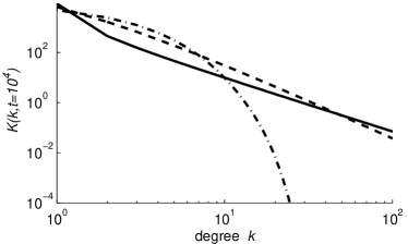
Figure 1 shows the numerical solution of these equations for different values of $q$. First, for $q=0.0$, it can be seen that the degree distribution is exponential. This is because for this value, the growth of the tree is equivalent to a fully random network. For larger values of $q$, the preferential attachment term has an increasing weight. The curves for $q=0.5$ and $q=0.9$ show that asymptotically (i.e. for large values of $k$) the distribution approaches a scale-free behaviour. The limit case $q=1$, however evolves into a star as nodes with degree $k=1$ can never be chosen as target of a new node. Thus, the degree distribution for this case is simply: $K(t-1,t)=1$, $K(1,t)=t-1$. This fact causes the dent in fgure 1 for $q=0.9$ at $k=1$.

Figure 1: Degree distribution $K(k,t)$ at $t=10^{4}$ for different values of $q$ obtained by recourse of iteration of the discrete equations (2-3.1.1). The different lines correspond to: $q=0.0$ (dash-dotted), $q=0.5$ (dashed) and $q=0.9$ (solid). The plot shows that for increasing values of $q$, the distribution is approaches a power law. The extreme case $q=1$ corresponds to a star, with the root having $k=t-1$ and all other nodes having $k=1$.

3.1.2 Closed forms

As pointed out in Ref [18], the model constitutes a particular case of the network growth model developed in Ref. [23], given that only one link is added each time step. The authors of Ref. [23] also derived a closed form for the stationary degree distribution in the limit in infinitely large networks (i.e. when $t\to\infty$). From this, we can infer the time dependent degree distribution. We substitute the variables used in Ref. [23] by the ones used in Ref [18] as follows: $m=1$ and $a=1+1/q$. The result is

$$\frac{K(k,t)}{t}=\frac{1}{q}\frac{\Gamma(2q^{-1}-1)}{\Gamma(q^{-1}-1)}\frac{\Gamma(k-1+q^{-1})}{\Gamma(k+2q^{-1})}.$$ (5)

We use $\Gamma$ to denote the Gamma function. For large values of $k$ the asymptotic limit of the distribution is

$$K(k)\propto k^{-(1+q)/q}.$$ (6)

While solving equations in the limit of infinitely large networks is a common practice in the field of complex networks, one must be cautious when dealing with real data. The question is whether or not the systems is large enough to justify the assumption $N\to\infty$. For example, real directory structures analysed contain between $10^{2}$ and $10^{5}$ nodes.

We have empirically computed the deviation of the numerical solution of equations (2–3.1.1) from the limit distribution defined by Eq. 6. The deviation is strongest for low values of $q$, i.e. $q=0$ is the worst case scenario. Figure 2 shows how the thermodynamic limit is approached for the case $q=0.1$ (Eq. 6 is undefined for $q=0$) for networks of coparable sizes to those found in our data ($10^{2}$ and $10^{5}$). The lines $K(k,t)/N=10^{-2}$ and $K(k,t)/N=10^{-5}$ are marked to indicate the areas relevant for estimating $q$ for these trees.

Figure 2: Comparison of the normalised degree distribution $K(k,t)/N$ for $q=0.1$ for different system sizes with the asymptotic behaviour of the degree distribution in the thermodynamic limit (cf. Eq. 6), depicted with solid line. The different system sizes are: $N=10^{2}$ (dash-dotted) and $N=10^{5}$ (dashed). Eq. (6) matches Eqs. (2–3.1.1) in the relevant regions $K(k,t)/N\geq 10^{-2}$ and $K(k,t)/N\geq 10^{-5}$ (dotted lines).

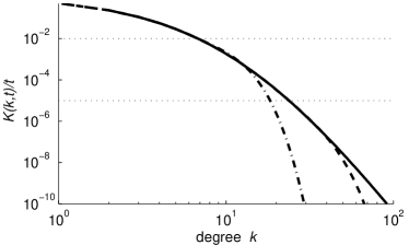
To test whether Eq. 6 is a sufficient approximation, there must not be a deviation between Eq. 6 and the Eqs. (2–3.1.1) at values larger than $t^{-1}$. It can be seen that the degree distribution found for small system sizes are such that the limit case is still a good approximation of the distribution found for real systems: The curve for the system size $N=10^{2}$ matches Eq. 6 for $K(k,t)/N\geq 10^{-2}$. Also for $N=10^{5}$ the limiting case is a good approximation for $K(k,t)/N\geq 10^{-5}$. Effectively, the finite-size effects are only observed with low probability and are all below the $K(k,t)=1$ line. For this reason, equation (5) could constitute an appropriate basis for estimating $q$ in a real data set.

3.1.3 Estimation of $q$ from the degree distribution

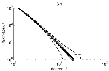
When fitting $q$ from the degree distribution of a single data set, it is important to bear in mind that equation (5) only describes the expected degree distribution (i.e. the one obtained after building the average of a large number of concrete tree manifestations). Particular realisations may deviate from it. Figure 3(a), shows (with points) the average value for the degree distribution over $10^{3}$ realisations of the tree obtained by numerical simulation. The dashed lines display the intervals in which 90% of the degree distributions lie. The expected values obtained via equation (5) are represented with circles. It can be seen that the intervals around the average values are relatively narrow.

In order to estimate the value of $q$ for a given tree of size $N$, one can proceed as follows. First, the degree distribution $K^{*}(k,t)$ of the tree, is measured. Then, this distribution is compared to the expected ones obtained through Eq. (5) for different values of $q$. The value $\bar{q}_{k}$ is the one whose associated degree distribution minimises the root mean square distance to the empirical $K^{*}(k,t)$.

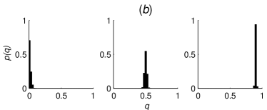
How accurate the estimation actually is, can be found by determining the specific error margins while estimating $q$ for a single tree. To do so, we generated $10^{4}$ different trees for each $q-$value: $q=0.0$, $q=0.5$ and $q=0.9$, and a system size $N=2\,500$. For each run, $q$ was estimated by fitting equation (5) with the least squares method described above. Figure 3(b) shows the distributions of the estimated values of $q$. In the case of $q=0.5$ the empirically estimated error margins for $q$ are $[0.48,0.53]$. Then, for $q=0.0$, the corresponding estimated error margins for $q$ are $[0.0,0.05]$. For $q=1.0$ the estimation is always exact as the only possible manifestation corresponds to a star. For this reason we analysed the case $q=0.9$ and found error margins of $[0.91,0.89]$. In all the cases, we set a confidence level of 90%. We can conclude that, using this method, the parameter $q$ can be well approximated by means of the degree distribution.

Figure 3: (a) Deviation of single simulated trees from the calculated degree distribution ($q=0.5$, $t=2\,500$). The solid line shows the mean of the simulations, circles the calculated mean, the dashed lines mark the tunnel in which 90% of the simulated trees lie. Panel (b): distribution of estimated values of $q$ by means of the degree distribution (see in-line text for details) for trees generated by computer simulations of the stochastic model described in Section 2. In the different plots: $q=0.0$ (left), $q=0.5$ (middle) and $q=0.9$ (right). The tree size is $N=2\,500$ and the distribution is based on $10^{4}$ simulation runs each.

3.2 Level distribution of nodes

At difference with what occurs in non-hierarchical networks, trees possess a special node, root, from which the tree starts its growth. Knowing the dynamics of the distribution of distances towards the root, unveils an alternative description of the process of tree growth. In this section, the evolution over time of this level distribution is solved. Moreover, it is shown that the equations describing the growth in terms of the level distribution are quite simple for the considered model, and allow for an independent estimation of the parameter $q$.

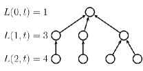
Let $L(l,t)$ be the number of nodes at distance $l$ to the root node at time $t$; i.e. $l$ defines the level of the node. From the set of the levels of all nodes, the level distribution of the tree can be compiled (for an illustration see figure 4).

Figure 4: Representation of the tree structure in terms of the level distribution: At level 0, there is only one node, the root. From it, the tree is grown with the stochastic model described in the text. The level distribution $L(l,t)$ is simply given by the number of nodes at a distance $l$ of the root. In the figure we represent each link with an arrow from child to parent.

3.2.1 Discrete description

In analogy to the recursive description of the degree distribution in section 3.1.1, we forumulate recursive equations for the level distribution:

$$L(l,1) = \delta_{l,0}$$ (7)

$$L(0,t) = 1$$ (8)

$$L(l,t) = L(l,t\!-\!1)$$

$$+(1-q)\frac{L(l\!-\!1,t\!-\!1)}{t}+q\frac{L(l,t\!-\!1)}{t},l\geq 1.$$

First, equation (7) refers to the initial condition of system in which only one node exists at level zero. Equation (8) explicits the condition of uniqueness of the root node over time. To understand Eq. (3.2.1) keep in mind that, adding a node at level $l$ means that a node at level $l-1$ was selected as parent. The first non-trivial term – the one preceded by the factor $(1-q)$ – corresponds to the process of random attachment. When nodes are selected at random, this term is proportional to $L(l-1,t)$. The last term represents the preferential attachment part, which occurs with probability $q$. To explain it, one has to consider that the probability to attach a new node to an existing one in level $l-1$ is proportional to the sum of the in-degrees on level $l-1$. Interestingly, in a tree, the sum of the in-degrees on level $l-1$ is equal to the number of nodes in the next level, i.e. $L(l,t)$.

Figure 5: Level distribution $L(l,t)$ at $t=10^{4}$ for different values of $q$ obtained by recourse of iteration of the discrete equations (7-3.2.1). The different lines correspond to: $q=0.0$ (dash-dotted), $q=0.5$ (dashed) and $q=0.9$ (solid). The plot shows that for increasing values of $q$, the distribution is sharper, corresponding to flatter structures and the average level approaches $l=1$. The extreme case $q=1$ corresponds to a star, with the root node as centre.

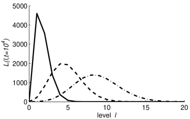
Figure 5 shows the expected level distributions obtained by direct integration of Eqs. (7–3.2.1) for different values of $q$ at time $t=10^{4}$. By increasing $q$, the distribution shifts closer to the root, and the tree is more shallow. In the limiting case of $q=1$, the tree takes the form of a star with the root at level zero and all the other nodes at level 1. Lower values of $q$ produce a broader level distribution, generating deeper trees. The influence of time (not shown in the figure) is straight-forward: The larger a tree grows, the higher the average node depth will be. This effect is stronger for lower values of $q$. In the next section we investigate the closed forms description of this relationship.

3.2.2 Closed forms

In order to take a closer look at the influence of $t$ on the level distribution, it is needed to solve the set of Eqs. (7-3.2.1), which define its evolution. In particular it is possible to derive closed forms for the extreme cases $q=1$ and $q=0$.

First, the case of $q=1$ is trivial: it produces a star with the root node as centre and the $N-1$ other nodes located at level 1, i.e.

$$L(0,t)=1\,;\,\,\,L(1,t)=t-1.$$ (10)

The average level $\langle L(l,t)\rangle=1-1/t$ in this case, approaches the constant value 1 for large enough trees.

Second, by rewriting the discrete time $t$ into the continuous limit, the following differential equation represents the case $q=0$:

$$\frac{dL(l,t)}{dt}=\frac{L(l-1,t)}{t}.$$ (11)

The initial condition is $L(0,1)=\delta_{1,l}$. As $L(l,t)$ does not appear on the right hand side of the differential equation the solution for level $l$ can trivially be obtained by direct integration of the solution for level $l-1$, divided by $t$. The general solution is found to be

$$L(l,t) = \int_{1}^{t}\frac{L(l-1,\tau)}{\tau}d\tau=\frac{1}{l!}\left[\ln(t)\right]^{l}.$$ (12)

It is easy to see that, in order to obtain the normalised distribution, the normalisation constant is $N$, i.e. the number of nodes at time $t$. For any given time, the distribution corresponds to a Poisson distribution, with parameter $\ln(t)$. Thus, the average level for the distribution is $\langle L(l,t)\rangle=\ln(t)$ and the variance $\hbox{Var}(L(l,t))=\ln(t)$.

Thus, the broadest level distribution generated by this model has a mean that grows logarithmically in time.

3.2.3 Estimation of $q$ from the level distribution

Figure 6: Top: Deviation of single simulated trees from the calculated level distribution ($q=0.5$, $t=2\,500$). The solid line shows the mean of the simulations, circles the calculated mean, the dashed lines mark the tunnel in which 90% of the simulated trees lie. Bottom: Distribution of estimated q for simulations with $q=0.0$ (left), $q=0.5$ (middle) and $q=0.9$ (right). The tree size is $N=2\,500$ and the distribution is based on $10^{4}$ simulation runs each.

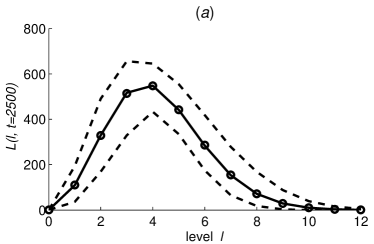
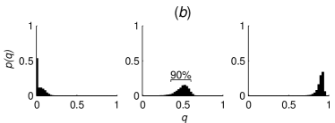
In a similar fashion as was done for the degree distribution, by means of equations (7–3.2.1) the expected level distributions can be calculated. Again, the level distribution obtained from a single realisation of the stochastic model in Section 2 might deviate from it. Panel (a) of figure 6 shows how large this deviation really is. For $10^{3}$ independent trees generated through simulations of the stochastic model, the dashed lines depict the interval in which 90% of the obtained level distributions lie. The broad intervals for the expected distribution suggest that estimating the parameter $q$ based on one tree instance might not be as accurate as the estimation based on the degree distribution.

Out of an empirically obtained level distribution of a tree with size $N$, the parameter $q$ is estimated as follows: First, the empirical level distribution $L^{*}(l,t)$ is measured. Then, this distribution is compared to the expected ones (Eqs. 7–3.2.1) obtained for different values of $q$ and the same integration time $t=N$. The estimated value $\bar{q}_{l}$ is the one whose associated level distribution minimises the root mean square distance to the empirical distribution $L^{*}(l,t)$.

It is important to know how the deviation of an estimated $q$ from the real value used to synthetically generate the tree according to the model (Section 2). This is done in analogy to the analysis of the estimation based on the degree distribution (see section 3.1.3). The growth model was simulated $10^{4}$ times for three different values of $q$: $q=0.0$, $q=0.5$ and $q=0.9$ and system size $N=2\,500$. Then, the value of $q$ was estimated according to the above algorithm. Figure 6 (panel (b)) shows the distributions of the estimated $q$. In the case of $q=0.0$ (left plot), 90% of the estimated values are in the interval $[0.0,0.13]$. In the case of $q=0.5$ (middle plot), 90% of the estimated values lie in the interval $[0.35,0.60]$, and $q=0.9$ (right plot) yields error margins of $[0.83,0.95]$. Finally, for the trees generated with $q=1.0$, the situation is similar to the one in section 3.1.3: the only possible tree is a star and thus $q$ is always correctly estimated.

Compared to the accuracy with which $q$ can be calculated from the degree distribution (see section 3.1.3) the level distribution turns out to be a less accurate indicator of $q$.

However, it is worth remarking that (if a tree is produced by the process introduced in Section 2) both estimations must agree quantitatively. In the next section, we test whether this is the case for user-generated directory structures.

4 Comparison of real-world data and model

In the previous theoretical investigations, we have represented the same model, equation (1), in terms of two different distributions, degree and level distribution. They can be seen as alternative ways of studying the same tree growth process. Thus, the two methods for computing the value of the parameter $q$ can be used to test whether the growth of a tree occurred following the studied model. Effectively, if the model is able to correctly reproduce the degree as well as the level distribution found in real directory structures, the $q$ calculated based on $L(l,t)$ should strongly correlate with the $q$ calculated based on $K(k,t)$.

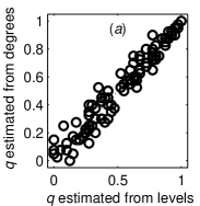
In Figure 7(a), the estimation of $q$ based on the level distribution (horizontal axis) and degree distribution (vertical axis) is shown for 100 trees generated by the model of Section 2. Each point corresponds to a tree of size $N=10^{3}$ and a value of $q$ uniformly drawn within the interval $[0,1]$. As expected, both measures are strongly correlated, and the points barely depart from the identity function.

In order to test whether the same applies to directory structures, we have collected $20$ user-generated directories corresponding to Linux/UNIX computer facilities. We have only considered directories as nodes of the network and did not include files or hard or soft links in the network. Also configuration directories (those with a leading dot, which are automatically generated either by the system or by particular programs) have been discarded, as they are not consciously generated by the user, and they present approximately the same structure for every user. With this, the trees obtained contain between $N=119$ and $N=75\,307$ directories (with median: $3467$).

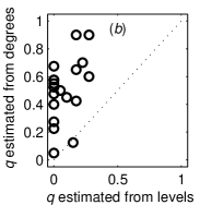
Figure 7(b) shows correlation between the two estimation methods when applied to the directory data collected. It can be seen that the correlation between the two measures is lost. Thus, the two estimated values of $q$ are incompatible with each other. This leads us to the conclusion that the model by Klemm et al. in its current state reproduces the degree distributions of directory structures quite well as shown in Ref. [18], but fails to produce the corresponding level distribution.

It is interesting to note that the parameter $q$ is wide spread, covering the range $[0,0.9]$ when estimating it by means of the degree distribution. This is in agreement with the experimental findings of Ref. [18], although in that reference an alternative Monte Carlo method was applied. However, when the level distribution is used to estimate the parameter $q$, the values found lay in the interval $[0,0.28]$. This implies that the tree structures found in real-world directory structures are much deeper than the predicted by the model.

It could be argued that the values of $q$ measured are lower because users might start their directory structure after a phony directory, such as the Desktop folder. Yet, performing the same regression analysis on shifted level distributions shows that in most of the cases the distribution must be shifted 3 or more levels in order to improve the correlation between both estimators of $q$. Such shifts, it is important to remark, are unrealistic in this context.

Figure 7: In both plots, we compare the values of $q$ estimated through the fitting of the level distribution (on the horizontal axis), with the estimation of $q$ obtained by means of the degree distribution (in the vertical axis). Panel (a) shows such a comparison for trees obtained by direct simulation of the stochastic growth model introduced in Section 2. The plot consists of $100$ trees with values of $q$ in the range $[0,1]$ and size $10^{3}$. In this plot it is apparent a good agreement between the two independent measures of the parameter $q$. Panel (b) shows the results obtained when analysing $20$ real directory structures with sizes between $N=119$ and $N=75\,307$. Interestingly, in this case the correlation between the measures is lost.

5 Conclusions

In this paper we have investigated a stochastic growth model for trees, where a parameter $q$ interpolates between two limiting cases: random growth ($q=0$) and preferential attachment ($q=1$). This model has been previously used to model the evolution of user-generated directories [18, 19], in particular the properties of the degree distribution and allometric scaling.

In this paper we extend the current state of this research by means of three contributions:

(i) We propose an alternative way of estimating the parameter $q$ from data by fitting an analytical solution. We show that, even though finite size effects exist, the solution proposed in Ref [23] for the thermodynamic limit is sufficiently accurate to estimate $q$ analytically from the data. This approach is more efficient than the computation intensive approach used in Ref [18].

(ii) We introduce the concept of level distribution as an important characterisation of trees. We argue that in order to verify a tree growth model, in addition to the degree distribution also the level distribution has to be taken into account. A model can claim evidence only if both of these independent representations are matched by the data. In the particular case of the stochastic growth model described above, it means that both ways should lead to the same estimation of the parameter $q$.

(iii) Applying our results for the degree and the level distribution to both simulated and user generated data, we find a perfect correlation between the estimated $q$ values for the simulated trees, but no correlation for the real-world user generated directories. Hence, we have to conclude that the growth of real directory trees are not sufficiently captured by the model given in [18]. In particular, user directories extend more in depth than the model predicts.

Our contributions also highlight that an analysis proven to be of relevance for complex networks does not necessarily give the full description of hierarchical structures, be they real or simulated. Thus, different aspects (or complementary descriptions, as was done in this Paper) must be studied in order to fully characterise these structures.

Acknowledgement: We want to thank the anonymous users who run our script to provide us with data on their directory structures. CJT acknowledges financial support from SBF (Swiss Confederation) through research project C05.0148 (Physics of Risk).

References

- [1] G. Caldarelli, Scale–Free Networks (Oxford University Press, 2007)
- [2] I. Rodríguez-Iturbe, A. Rinaldo, Fractal River Basins: Chance and Self-Organization (Cambridge University Press, 1997)
- [3] E. Weibel, American Journal of Physiology- Lung Cellular and Molecular Physiology 261(6), 361 (1991)
- [4] M. Zamir, Journal of Theoretical Biology 197(4), 517 (1999)
- [5] J.R. Banavar, A. Maritan, A. Rinaldo, Nature 399(6732), 130 (1999)
- [6] P. Prusinkiewicz, A. Lindenmayer, The algorithmic beauty of plants (Springer-Verlag New York, Inc. New York, NY, USA, 1990)
- [7] J. Cracraft, M. Donoghue, Assembling the Tree of Life (Oxford University Press, USA, 2004)
- [8] C. Dupuis, Annual Reviews in Ecology and Systematics 15(1), 1 (1984)
- [9] A. Rokas, Science 313, 1897 (2006)
- [10] E.A. Herrada, C.J. Tessone, V.M. Eguíluz, E. Hernández-García, C.M. Duarte, PLoS ONE 3, e2757 (2008)
- [11] E. Hernández-García, E.A. Herrada, A.F. Rozenfeld, C.J. Tessone, V.M. Eguíluz, C.M. Duarte, S. Arnaud-Haond, E. Serrão, Evolutionary and Ecological Trees and Networks, in XV Conference on Nonequilibrium Statistical Mechanics and Nonlinear Physics, edited by O. Descalzi, O.A. Rosso, H.A. Larrondo (AIP Conference Proceedings, 2007), Vol. 913, pp. 78–83
- [12] L. Muchnik, R. Itzhack, S. Solomon, Y. Louzoun, Physical Review E 76(1), 016106 ( 12) (2007)
- [13] D.A. Huffman, Proceedings of the IRE 40(9), 1098 (1952)
- [14] D. Knuth, The art of computer programming, volume 1: fundamental algorithms (Addison Wesley Longman Publishing Co., Inc. Redwood City, CA, USA, 1997)
- [15] M. Goodrich, R. Tamassia, Algorithm Design: Foundations, Analysis, and Internet Examples (J. Wiley, 2002)
- [16] S. Golder, B. Huberman, Journal of Information Science 32, 198 (2006)
- [17] E. Codd, Communications of the ACM 13(6), 377 (1970)
- [18] K. Klemm, V.M. Eguíluz, M. San Miguel, Physical Review Letters 95(12), 128701 ( 4) (2005)
- [19] K. Klemm, V.M. Eguíluz, M.S. Miguel, Physica D: Nonlinear Phenomena 224(1-2), 149 (2006)
- [20] P.L. Krapivsky, S. Redner, F. Leyvraz, Physical Review Letters 85(21), 4629 (2000)
- [21] D. Garlaschelli, G. Caldarelli, L. Pietronero, Nature 423, 165 (2003)
- [22] D. Garlaschelli, G. Caldarelli, L. Pietronero, Nature E4, 165 (2005)
- [23] S. Dorogovtsev, J. Mendes, A. Samukhin, Physical Review Letters 85(21), 4633 (2000)