Recursive algorithm for arrays of generalized Bessel functions:
Numerical access to Dirac-Volkov solutions

Abstract

In the relativistic and the nonrelativistic theoretical treatment of moderate and high-power laser-matter interaction, the generalized Bessel function occurs naturally when a Schrödinger-Volkov and Dirac-Volkov solution is expanded into plane waves. For the evaluation of cross sections of quantum electrodynamic processes in a linearly polarized laser field, it is often necessary to evaluate large arrays of generalized Bessel functions, of arbitrary index but with fixed arguments. We show that the generalized Bessel function can be evaluated, in a numerically stable way, by utilizing a recurrence relation and a normalization condition only, without having to compute any initial value. We demonstrate the utility of the method by illustrating the quantum-classical correspondence of the Dirac-Volkov solutions via numerical calculations.

I Introduction

The Volkov solution Volkov (1935) is the exact solution of the Dirac equation in the presence of a classical plane-wave laser field of arbitrary polarization. In order to evaluate cross sections by quantum electrodynamic perturbation theory, it is crucial to decompose the Volkov solutions into plane waves, in order to be able to do the time and space integrations over the whole Minkowski space-time. If the laser field is linearly polarized, one naturally encounters the generalized Bessel functions as coefficients in the plane-wave (Fourier) decomposition of the wave function, both for the Dirac-Volkov equation as well as for the laser-dressed Klein–Gordon solutions, and even for Schrödinger-Volkov states (see also Sec. V).

The wide use of the generalized Bessel function in theoretical laser physics is thus due to the fact that different physical quantities, such as scattering cross sections and electron-positron pair production rates, can be expressed analytically in terms of infinite sums over generalized Bessel functions which we here denote by the symbol $J_{n}(x,y)$. The generalized Bessel function $J_{n}(x,y)$ is a generalization of the ordinary Bessel function $J_{n}(x)$ and characteristic of the interaction of matter with a linearly polarized laser field; it depends on two arguments $x$ and $y$, and one index $n$. Here, we use it in the convention

$$\begin{split}J_{n}(x,y)=\frac{1}{2\pi}\int_{-\pi}^{\pi}\exp[-\mathrm{i}\,n\,\theta&+\mathrm{i}\,x\,\sin(\theta)\\ &-\mathrm{i}\,y\,\sin(2\theta)]\,\mathrm{d}\theta,\end{split}$$ (1)

where $n$ is an integer, and $x$ and $y$ are real numbers. $J_{n}(x,y)$ is real valued. The generalized Bessel functions provide a Fourier decomposition for expressions of the form $\exp\left[\mathrm{i}\,x\,\sin\theta-\mathrm{i}\,y\,\sin(2\theta)\right]$ as follows,

$$\exp\left[\mathrm{i}\,x\,\sin\theta-\mathrm{i}\,y\,\sin(2\theta)\right]=\sum_{n=-\infty}^{\infty}\,J_{n}(x,y)\,\exp\left(\mathrm{i}\,n\,\theta\right)\,.$$ (2)

In practical applications, the angle $\theta$ often has the physical interpretation of a phase of a laser wave, $\theta=\omega\,t-\vec{k}\cdot\vec{x}$, where $\omega$ is the angular laser photon frequency, and $\vec{k}$ is the laser wave vector. By contrast, the well-known ordinary Bessel functions are defined as

$$J_{n}(x)=\frac{1}{2\pi}\int_{-\pi}^{\pi}\exp\left[-\mathrm{i}\,n\,\theta+\mathrm{i}\,x\,\sin(\theta)\right]\,\mathrm{d}\theta\,,$$ (3)

and they have the fundamental property

$$\exp\left(\mathrm{i}\,x\,\sin\theta\right)=\sum_{n=-\infty}^{\infty}\,J_{n}(x)\,\exp\left(\mathrm{i}\,n\,\theta\right)\,.$$ (4)

The generalized Bessel function was first introduced by Reiss in the context of electron-positron pair creation Reiss (1962), followed by work of Nikishov and Ritus Nikishov and Ritus (1964), and Brown and Kibble Brown and Kibble (1964). Further examples of work utilizing $J_{n}(x,y)$ in the relativistic domain include pair production by a Coulomb field and a laser field Mittleman (1987); Müller et al. (2004); Sieczka et al. (2006), laser-assisted bremsstrahlung Lötstedt et al. (2007); Schnez et al. (2007); Roshchupkin (1985), muon-antimuon creation Müller et al. (2008, 2008), undulator radiation Dattoli and Voykov (1993), and scattering problems, both classical Sarachik and Schappert (1970), and quantum mechanical Panek et al. (2002a, b). A fast and reliable numerical evaluation of $J_{n}(x,y)$ would also speed up calculation of wave packet evolution in laser fields Roman et al. (2000, 2003). In nonrelativistic calculations, the generalized Bessel function has been employed mainly for strong-field ionization Reiss (1980); Reiss and Krainov (2003); Vanne and Saenz (2007); Guo et al. (2008), but also for high-harmonic generation Gao et al. (1998, 2000).

On the mathematical side, a thorough study of $J_{n}(x,y)$ has been initiated in a series of papers Dattoli et al. (1990, 1991, 1993), and even further generalizations of the Bessel function to multiple arguments and indices have been considered Dattoli et al. (1995, 1998); Korsch et al. (2006); Klumpp et al. (2007). On the numerical side, relatively little work has been performed. Asymptotic approximations have been found for specific regimes Nikishov and Ritus (1964); Reiss (1980), and a uniform asymptotic expansion of $J_{n}(x,y)$ for large arguments by saddle-point integration is developed in Ref. Leubner (1981). For some of the applications described above, in particular when evaluating second-order laser-assisted quantum electrodynamic processes Lötstedt et al. (2009), a crucial requirement is to evaluate large sets of generalized Bessel functions, at fixed arguments $x$ and $y$, for all indices $n$ for which the generalized Bessel functions acquire values which are numerically different from zero (as we shall see, for $|n|\gg|x|,|y|$, the generalized Bessel functions decay exponentially with $n$).

It is clear that recursions in the index $n$ would greatly help in evaluating large sets of Bessel functions. For ordinary Bessel functions, an efficient recursive numerical algorithm is known, and it is commonly referred to as Miller’s algorithm Bickley et al. (1960); Gautschi (1967). However, a generalization of this algorithm for generalized Bessel functions has been lacking. The purpose of this paper is to provide such a recursive numerical algorithm: We show, using ideas from Oliver (1968a); Mattheij (1980, 1982); Wimp (1984), that a stable recurrence algorithm can indeed be established, despite the more complex recurrence relation satisfied by $J_{n}(x,y)$, as compared to the ordinary Bessel function $J_{n}(x)$. The reduction of five-term recursions to four- and three-term recursions proves to be crucial in establishing a numerically stable scheme.

The computational problem we consider is the following: to evaluate

$$J_{n}(x,y):\quad x\,\,\mbox{fixed},\quad y\,\,\mbox{fixed}\,,$$

$$\mbox{where}\quad n_{\textrm{min}}\leq n\leq n_{\textrm{max}}\,,$$ (5)

by recursion in $n$. Our approach is numerically stable, and while all algorithms described here have been implemented in quadruple precision (roughly 32 decimals), we note that the numerical accuracy of our approach can easily be increased at a small computational cost.

Our paper is organized as follows. In Sec. II, we recall some well-known basic properties of $J_{n}(x,y)$, together with some properties of the solutions complementary to $J_{n}(x,y)$, which fulfill the same recursion relations (in $n$) as the generalized Bessel functions but have a different asymptotic behavior for large $|n|$ as compared to $J_{n}(x,y)$. After a review of the Miller algorithm for the ordinary Bessel function, we present a recursive Miller-type algorithm for generalized Bessel functions in Sec. III, and show that it is numerically stable. In Sec. IV, we numerically study the accuracy which can be obtained, and compare the method presented here with other available methods. We also complement the discussion by considering in Sec. V illustrative applications of the numerical algorithm for Dirac–Volkov solutions in particular parameter regions, together with a physical derivation of the recurrence relation satisfied by the generalized Bessel function. Section VI is reserved for the conclusions.

II Basic properties of the generalized Bessel function

II.1 Orientation

Because the definition (1) provides us with a convenient integral representation of the generalized Bessel function, all properties of $J_{n}(x,y)$ needed for the following sections of this article can in principle be derived from this representation alone Nikishov and Ritus (1964); Reiss (1980). E.g., shifting $\theta\to-\theta-\pi$ and $\theta\to\theta+\pi$, respectively, in (1) gives two symmetries,

$$\begin{split}J_{n}(x,-y)&=(-1)^{n}J_{-n}(x,y),\\ J_{n}(-x,y)&=(-1)^{n}J_{n}(x,y),\end{split}$$ (6)

from which $J_{-n}(x,y)=J_{n}(-x,-y)$ follows. We recall the corresponding properties of the ordinary Bessel function,

$$J_{n}(x)=(-1)^{n}J_{n}(-x)=(-1)^{n}J_{-n}(x)\,.$$ (7)

Due to the symmetries (6), we can consider in the following only the case of positive $x$ and $y$ without loss of generality, provided we allow $n$ to take arbitrary positive and negative integer values. Our sign convention for the $y\sin 2\theta$-term in the argument of the exponential in Eq. (1) agrees with Nikishov and Ritus (1964), but differs from the one used in Reiss (1980). As is evident from inspection of Eqs. (1) and (3), $J_{n}(x,y)$ can be expressed as an ordinary Bessel function if one of its arguments vanishes,

$$J_{n}(x,0)=J_{n}(x),\qquad J_{n}(0,y)=\left\{\begin{array}[]{ll}J_{-n/2}(y)&\textrm{if }n\textrm{ even}\\ 0&\textrm{if }n\textrm{ odd}.\end{array}\right.$$ (8)

By inserting the expansion of the ordinary Bessel function $\sum_{n=-\infty}^{\infty}J_{n}(x)\exp(in\theta)=\exp(\mathrm{i}\,x\,\sin\theta)$ into Eq. (1), we see that $J_{n}(x,y)$ can be expressed as an infinite sum of products of ordinary Bessel function,

$$J_{n}(x,y)=\sum_{s=-\infty}^{\infty}J_{2s+n}(x)J_{s}(y).$$ (9)

There are also the following sum rules,

$$\sum_{n=-\infty}^{\infty}J_{n}(x,y)=\sum_{n=-\infty}^{\infty}J_{n}^{2}(x,y)=1\,,$$ (10)

which can be derived by considering the case $\theta=0$ in Eq. (2) [for $\sum_{n=-\infty}^{\infty}J_{n}(x,y)=1$], and by considering Eq. (2) multiplied with its complex conjugate, and integrating over one period [for $\sum_{n=-\infty}^{\infty}J_{n}^{2}(x,y)=1$]. The relation (10) is important for a recursive algorithm, because it provides a normalization for an array of generalized Bessel function computed according to the recurrence relation

$$\begin{split}&2nJ_{n}(x,y)=x\,\left[J_{n+1}(x,y)+J_{n-1}(x,y)]\right.\\ &\qquad\left.-2y\,[J_{n+2}(x,y)+J_{n-2}(x,y)\right]\,,\end{split}$$ (11)

which connects generalized Bessel functions of the same arguments but different index $n$. Equation (11) can be derived by partial integration of Eq. (1). Interestingly, Eq. (11) together with the normalization condition (10) can be taken as an alternative definition for $J_{n}(x,y)$, from which the integral representation (1) follows. The recursion (11) is the basis for the algorithm described below in Sec. III.

II.2 Saddle point considerations

A qualitative picture of the behavior of $J_{n}(x,y)$ as a function of $n$ can be obtained by considering the position of the saddle points of the integrand in (1) Leubner (1981); Korsch et al. (2006). By definition, a saddle point $\theta_{s}$ denotes the point where the derivative of the argument of the exponential in (1) vanishes, and therefore satisfies

$$\cos\theta_{s\pm}=\frac{x}{8y}\pm\sqrt{\frac{x^{2}}{64\,y^{2}}+\frac{1}{2}-\frac{n}{4y}}.$$ (12)

By writing $J_{n}(x,y)$ as

$$\begin{split}J_{n}(x,y)=\frac{1}{\pi}\mathrm{Re}\Bigg{\{}\int_{0}^{\pi}\exp[-\mathrm{i}\,n\,\theta&+\mathrm{i}\,x\,\sin(\theta)\\ &-\mathrm{i}\,y\,\sin(2\theta)]\,\mathrm{d}\theta\Bigg{\}},\end{split}$$ (13)

we can consider only saddle points with $0\leq\mathrm{Re}\,\theta_{s}\leq\pi$. By the properties of the cosine function, the saddle points come in conjugate pairs, so that if $\theta_{s}$ is a saddle point, so is $\theta_{s}^{\ast}$. Furthermore, since $\cos(2\pi-\theta_{s})=\cos\theta_{s}$, the saddle points are placed mirror symmetrically around $\mathrm{Re}\,\theta_{s}=\pi$. Since each of the endpoint contributions at $\theta=0$ and $\theta=\pi$ to the integral (13) vanish (provided the endpoints are not saddle points), an asymptotic approximation for $J_{n}(x,y)$ is provided by the saddle point method (the method of steepest descent) Olver (1997), by summing the contributions from the saddle points $\theta_{s}$ situated on the path of steepest descent. Here, imaginary saddle points (i.e., saddle points with ${\rm Im}\,\theta_{s\pm}\neq 0$) give exponentially small contributions to the integral, while real saddle points contribute with an oscillating term. Closer inspection of Eq. (12) reveals two cases.

In case 1, with $8y>x$, there are four different regions, which we denote by $a_{1},b_{1},c_{1},d_{1}$ (see Table 1). In region $a_{1}$, where $n<-2y-x$, we have four distinct saddle points solutions $\theta_{s\pm}$, $\theta_{s\pm}^{\ast}$, which are all imaginary, and $J_{n}(x,y)$ is exponentially small. Region $b_{1}$, where $-2y-x<n<-2y+x$, has two imaginary ($\theta_{s+}$, $\theta_{s+}^{\ast}$) and one real saddle point $\theta_{s-}$, and $J_{n}(x,y)$ exhibits an oscillating behavior here. For $-2y+x<n<2y+x^{2}/(16y)$, i.e. in region $c_{1}$, both saddle points are real, and in the region $d_{1}$, $n>2y+x^{2}/(16y)$, the two saddle points $\theta_{s\pm}$ are again imaginary, which results in very small numerical values of the generalized Bessel functions. For case 2, $8y<x$, there are only three regions, as recorded in Table 1. The two cases coincide if $8y=x$. Figure 1 illustrates the two different cases.

Table 1: Saddle-point configurations for the generalized Bessel function $J_{n}(x,y)$ as a function of the arguments $x$ and $y$. A distinct imaginary saddle point is denoted “imag.” whereas a real saddle point is denoted “real.” The different regions are illustrated in Fig. 1.

Case 1: $8y>x$
region	condition	saddle points
$a_{1}$	$n<-2y-x$	4 imag.
$b_{1}$	$-2y-x<n<-2y+x$	2 imag.$+$real
$c_{1}$	$-2y+x<n<2y+x^{2}/(16y)$	2 real
$d_{1}$	$n>2y+x^{2}/(16y)$	2 imag.
Case 2: $8y<x$
region	condition	saddle points
$a_{2}$	$n<-2y-x$	4 imag.
$b_{2}$	$-2y-x<n<-2y+x$	2 imag.$+$real
$c_{2}$	$n>-2y+x$	2 imag.

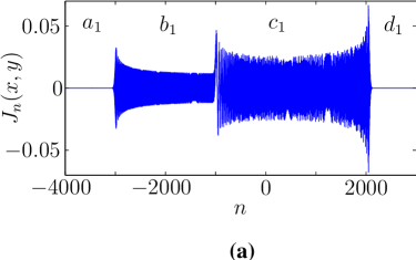
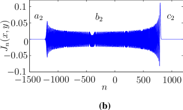
Figure 1: (Color online.) Illustration of the different saddle point regions of $J_{n}(x,y)$, for the two qualitatively different cases number 1, with $8y>x$ (here $x=y=10^{3}$ was used), and case number 2, with $8y<x$ ($x=10y=10^{3}$). In case 1 [panel (a)], the transition from region $b_{1}$, where only one saddle point is real, to $c_{1}$, where two real saddle points contribute, occurs precisely at $n=-2y+x=-10^{3}$ (see also Table 1). The complex oscillating behavior in region $c_{1}$ can be understood as interference between the contributions from the two real saddle points. In case 2 [panel (b)], we have $8y<x$, with only three as opposed to four qualitatively different regions (see also Table 1).

In all regions $a_{1},b_{1},c_{1},d_{1},a_{2},b_{2},c_{2}$, there are, depending on the region, up to four saddle points to consider. Of these one or two saddle points contribute to the numerical approximation to $J_{n}(x,y)$. For large arguments $y$, $x$ and/or a large index $n$, asymptotic expressions can be derived Leubner (1981); Korsch et al. (2006). The general form for the leading-order term is (see Olver (1997) for a clear exposition of the general theory of asymptotic expansions of special functions)

$$\begin{split}&J_{n}(x,y)\\ &\approx\mathrm{Re}\left[\sqrt{\frac{2}{\pi|f^{\prime\prime}(\theta_{s+})|}}\,\exp\left(\mathrm{i}f(\theta_{s+})-\mathrm{i}\,n\,\theta_{s+}+\mathrm{i}\varepsilon_{+}\right)\right.\\ &\quad\left.+\sqrt{\frac{2}{\pi|f^{\prime\prime}(\theta_{s-})|}}\,\exp\left(\mathrm{i}f(\theta_{s-})-\mathrm{i}\,n\,\theta_{s-}+\mathrm{i}\varepsilon_{-}\right)\right]\\[8.61108pt] &=F_{+}(n,x,y)+F_{-}(n,x,y),\end{split}$$ (14)

where

$$f(\theta)=x\sin(\theta)-y\sin(2\theta)\,.$$ (15)

For imaginary saddle points, only the contribution of those situated on the path of steepest descent should be included , i.e., the integration around the saddle point should be carried out along a curve of constant complex phase, with $\theta=\mu+i\nu$ satisfying

$$\mathrm{Im}\left(\mathrm{i}f(\theta)-\mathrm{i}\,n\,\theta\right)=\mathrm{const.}$$ (16)

on that curve. In practice this means for regions with imaginary saddle points only, $J_{n}(x,y)$ is given by the contribution from the saddle point with smallest $|\mathrm{Im}\,\theta_{s}|$, and in regions with both imaginary and real $\theta_{s}$ the contribution from the imaginary saddle point can be neglected. However, we will see in the following discussion that all saddle points, including those not on the path of steepest descent which would produce an “exponentially large” contribution, can be interpreted in terms of complementary solutions to the recurrence relation (11). The constant phase $\varepsilon_{\pm}$ in Eq. (14) is given by

$$\varepsilon_{\pm}=\frac{\pi}{4}\,{\rm sgn}\left[f^{\prime\prime}(\theta_{s\pm})\right]$$ (17)

for real saddle points. For imaginary saddle points, $\varepsilon_{\pm}$ can be found from the requirement

$$\tan\varepsilon_{\pm}=\left.\frac{d\nu}{d\mu}\right|_{\theta=\theta_{s\pm}},$$ (18)

with $\theta=\mu+i\nu$ describing the path of steepest descent [see Eq. (16)]. For a detailed treatment of the saddle point approximation of $J_{n}(x,y)$ we refer to Leubner (1981), where uniform approximations, valid also close to the turning points (the borders between the regions described in Fig. 1), and beyond the leading term (14), are derived. For our purpose, namely to identify the asymptotic behavior of the complementary solutions, the expression (14) is sufficient.

II.3 Complementary solutions

The recurrence relation (11) involves the five generalized Bessel functions of indices $n-2,n-1,n,n+1,n+2$. In general, an $m$-term recursion relation is said to be of order $m-1$. If we regard the index $n$ as a continuous variable, then a recursion relation of order $m-1$ corresponds to a differential equation of order $m-1$, which has $(m-1)$ linearly independent solutions. Equation (11) consequently has four linearly independent (complementary) solutions. The function $J_{n}(x,y)$ is one of these.

For the analysis of the recursive algorithm in Sec. III below, we should also identify the complementary solutions to the recurrence relation (11). For our purposes, it is sufficient to recognize the asymptotic behavior of the complementary solutions in the different regions $a_{1}$–$d_{1}$ and $a_{2}$–$c_{2}$ (see Fig. 1). It is helpful to observe that the recurrence relation (11) is satisfied asymptotically by each term $F_{\pm}(n,x,y)$ from Eq. (14) individually. The recurrence relation (11) is also satisfied, asymptotically, by a function obtained by taking in Eq. (14) a saddle point that is not on the path of steepest descent, which is equivalent to changing the sign of the entire argument of the exponential. In addition, for real saddle points and in regions with only two imaginary saddle points, the recurrence relation is asymptotically satisfied by taking the same saddle point but the imaginary part instead of the real part in Eq. (14) (and thereby changing the phase).

In regions with four imaginary saddle points ($a_{1},a_{2}$), there are thus two solutions that are exponentially increasing with the index $n\to-\infty$ [the two solutions correspond to the two saddle points $\theta_{s}$ where $\mathrm{Re}(\mathrm{i}f(\theta_{s})-\mathrm{i}n\theta_{s})>0$], and two further solutions which are exponentially decreasing [From $\theta_{s}$ with $\mathrm{Re}(\mathrm{i}f(\theta_{s})-\mathrm{i}n\theta_{s})<0$]. In regions with two imaginary and one real saddle point ($b_{1},b_{2}$), the four solutions behave as follows. There are two oscillatory solutions [these correspond to the real and imaginary parts of the term which contains the real saddle point in Eq. (14)], and a third solution which is exponentially increasing, and a fourth one which is exponentially decreasing as $n\to-\infty$ [the two latter solutions are due to the imaginary saddle points in Eq. (14)]. The region with two real saddle points ($c_{1}$) has four oscillating solutions, as a function of $n$. Finally, in regions $d_{1}$ and $c_{2}$, where we have two distinct imaginary saddle points, we have two exponentially increasing (as $n\to\infty$) solutions with different phase, and two exponentially decreasing with different phase. Concerning the question of how to join the different asymptotic behaviors to form four linearly independent solutions, we note that $J_{n}(x,y)$ is the only solution which can decrease in both directions $n\to\pm\infty$, since it represents the unique, normalizable physical solution to the wave equation (see subsection V.1). Furthermore, there must be one solution that increases exponentially where $J_{n}(x,y)$ decreases, and that exhibits an oscillatory behavior where $J_{n}(x,y)$ also oscillates. The reason is that in either of the limits $x\to 0$ or $y\to 0$, we must recover the ordinary Bessel function, and the Neumann function as the two solutions to the recurrence relation. Having fixed the asymptotic behavior of two of the solutions, the behavior of the the two remaining functions follows. We label the four different solutions with $J_{n}$, $Y_{n}$, $X_{n}$, and $Z_{n}$, where $J_{n}$ is the generalized Bessel function $J_{n}(x,y)$ with the arguments $x$, $y$ suppressed.

Integral representations for the complementary solutions can be found by employing Laplace’s method Jordan (1960), details of which will be described elsewhere. The explicit expressions can be found in the Appendix. However, as noted previously, in this paper we shall need only the asymptotic properties of the complementary solutions, which can be deduced from (14).

We also observe that the situation for $J_{n}(x,y)$ described above is directly analogous to that of the ordinary Bessel function $J_{n}(x)$ and the complementary Neumann (also called Weber) function $Y_{n}(x)$ of a single argument. For $x\gg n$ they have the asymptotic behavior $J_{n}(x)\approx\mathrm{Re}\,\sqrt{2/(\pi x)}\exp(\mathrm{i}x-\mathrm{i}\pi/4-\mathrm{i}n\pi/2)$, $Y_{n}(x)\approx\mathrm{Im}\,\sqrt{2/(\pi x)}\exp(\mathrm{i}x-\mathrm{i}\pi/4-\mathrm{i}n\pi/2)$, and for $x\ll n$ we have $J_{n}(x)\approx(\mathrm{e}x)^{n}(2n)^{-n}/\sqrt{2\pi n}$, $Y_{n}(x)\approx-2(\mathrm{e}x)^{-n}(2n)^{n}/\sqrt{2\pi n}$.

According to the above discussion and as illustrated in Fig. 2, the functions $J_{n}$, $Y_{n}$, $X_{n}$, and $Z_{n}$ have the following relative amplitudes in the different regions:

$$\begin{array}[]{ll}\textrm{region }a_{1},a_{2}:&|Z_{n}|>|Y_{n}|>|J_{n}|>|X_{n}|,\\ \textrm{region }b_{1},b_{2}:&|Z_{n}|>|Y_{n}|\sim|J_{n}|>|X_{n}|,\\ \textrm{region }c_{1}:&|Z_{n}|\sim|Y_{n}|\sim|J_{n}|\sim|X_{n}|,\\ \textrm{region }d_{1},c_{2}:&|Y_{n}|\sim|X_{n}|>|J_{n}|\sim|Z_{n}|.\end{array}$$ (19)

In Eq. (19), we have assumed that all functions have the same order of magnitude in the oscillating region. This can be accomplished by choosing a suitable constant prefactor for the complementary functions $Z_{n}$, $Y_{n}$, and $X_{n}$. Figure 2 shows an example of the four different solutions, for case 1 ($8y>x$). The actual numerical computation of the complementary solutions is discussed in Sec. III.3.

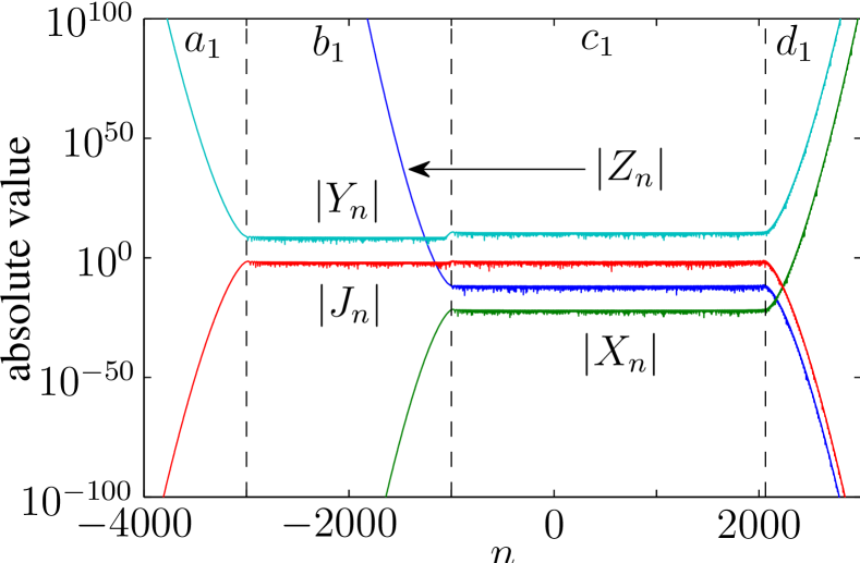
Figure 2: (Color online.) The five-term recurrence relation (11) has four linearly independent solutions. Note the logarithmic scale. The values $x=y=10^{3}$ were used for the calculation, corresponding to case 1 ($8y>x$). The solutions are labeled by $J_{n}$ [red line, the true generalized Bessel function $J_{n}(x,y)$], $Y_{n}$ (light blue line), $X_{n}$ (green line), and $Z_{n}$ (blue line). The numerically obtained solutions $X_{n}$, $Y_{n}$, and $Z_{n}$ have been shifted vertically by multiplication with an appropriate constant (of order $10^{10}$ for $Y_{n}$, $10^{-10}$ for $Z_{n}$, and $10^{-20}$ for $X_{n}$) for clarity. The separation of the different saddle point regions is marked with dashed lines. The regions $a_{1},b_{1},c_{1}$ and $d_{1}$ are described in Table 1.

III Miller–Type algorithm for generalized Bessel functions

III.1 Recursive Miller’s algorithm for ordinary Bessel functions

A straightforward implementation of Miller’s algorithm Bickley et al. (1960); Gautschi (1967); Mohr (1974) can be used for the numerical calculation of the ordinary Bessel function $J_{n}(x)$. We note that there are also other ways of numerically evaluating $J_{n}(x)$, which include series expansions Watson (1962) or contour integration Matviyenko (1993). In the following, we review the simplest form of Miller’s algorithm, to prepare for the discussion on the generalized algorithm. We treat the case of positive $n$ and $x$. For negative $n$ and $x$, we appeal to the symmetry relation (7). The properties of $J_{n}(x)$ used for the algorithm are the recurrence relation (11), with $y=0$, which automatically reduces (11) to a three-term relation with only two linearly independent solutions. We also use the normalization condition $\sum_{n=-\infty}^{\infty}J_{n}(x)=1$.

Viewed as a function of $n$, $J_{n}(x)$ exhibits an oscillatory behavior for $n<x$, and decreases exponentially for $n>x$. The complementary solution $Y_{n}(x)$, called the Neumann function, oscillates for $n<x$ and grows exponentially for $n>x$. To calculate an array of $J_{n}(x)$, for $0\leq n<N$, with $N>x$, we proceed as follows. We take a (sufficiently large) integer $M>N$, and the initial values $c_{M}=1$, $c_{M+1}=0$. We use the recurrence relation (11) with $y=0$ to calculate all $c_{n}$ with indices $0\leq n<M$ by downward recursion in $n$. Now, since the ensemble of the $Y_{n}(x)$ plus the $J_{n}(x)$ constitute a complete basis set of functions satisfying the recurrence relation, the computed array of the $c_{n}$ can be decomposed into a linear combination,

$$c_{n}=\alpha\,J_{n}(x)+\beta\,Y_{n}(x)\,,$$ (20)

where $\alpha$ and $\beta$ are constants, and this decomposition is valid for any $n$. That means that the same decomposition must also be valid for the initial index $M+1$ from which we started the downward recursion, i.e.

$$c_{M+1}=0=\alpha\,J_{M+1}(x)+\beta\,Y_{M+1}(x).$$ (21)

From Eq. (20) it follows that

$$c_{n}=\alpha\,\left(J_{n}(x)-\frac{J_{M+1}(x)\,Y_{n}(x)}{Y_{M+1}(x)}\right)\,.$$ (22)

Provided the starting index $M>x$ is chosen large enough, the quantity $J_{M+1}(x)/Y_{M+1}(x)$ is a small quantity, due to the exponential character of $J_{n}(x)$ and $Y_{n}(x)$ for index $n>x$, so that the computed array $c_{n}$ is to a good approximation proportional to the sought $J_{n}(x)$. Loosely speaking, we can say that we have selected the exponentially decreasing function $J_{n}(x)$ by the downward recursion, because the exponentially increasing function $Y_{n}(x)$ as $|n|\to\infty$ is suppressed in view of its exponential decrease for decreasing $|n|$. In other words, the error introduced by the initial conditions decreases rapidly due to the rapid decrease of $Y_{n}(x)$ for decreasing $n$, so that effectively only the part proportional to $J_{n}(x)$ is left.

Finally, the constant $\alpha$ can be found by imposing the normalization condition

$$\sum_{n}c_{n}=c_{0}+2\sum_{n=1}^{\infty}c_{2n}=1.$$ (23)

Here, we have used the symmetries (7) in order to eliminate the terms of odd index from the sum.

Remarkably, numerical values of $J_{n}(x)$ can be computed by using only the recurrence relation and the normalization condition, and not a single initial value is needed [e.g., one might otherwise imagine $J_{0}(x)$ to be calculated by a series expansion]. Miller’s algorithm has subsequently been refined and the error propagation analyzed by several authors Gautschi (1967); Olver (1964); Oliver (1967); Olver and Sookne (1972), and also implemented Ratis and Fernández de Córdoba (1993); du Toit (1993); Yousif and Melka (1997).

III.2 Recursive algorithm for generalized Bessel functions

In view of the four different solutions pictured in Fig. 2, it is clear from the discussion in the preceding subsection that $J_{n}(x,y)$ cannot be calculated by naïve application of the recurrence relation. The general paradigm (see Fig. 2) therefore has to change. We first observe that if we would start the recursion using the five-term recurrence relation (11) in the downward direction, starting from large positive $n$, then the solution would eventually pick up a component proportional to $Z_{n}$, which diverges for $n\to-\infty$. Conversely, if we would start the recursion using the five-term recurrence relation (11) in the upward direction, starting from large negative $n$, then the solution would pick up a component proportional to $X_{n}$. Thus, Eq. (11) cannot be used directly.

The solution to this problem is based on rewriting (11) in terms of recurrences with less terms (only three or four as opposed to five). By consequence, the reformulated recurrence has less linearly independent solutions, and in fact it can be shown (see the discussion below) that the four-term recurrence, if used in the appropriate directions in $n$, numerically eliminates the most problematic solution $Z_{n}$ which would otherwise be admixed to $J_{n}(x,y)$ for $n\to\infty$, leading to an algorithm by which it is possible to calculate the generalized Bessel function $J_{n}(x,y)$ for $n$ down to the point where we transit from region $b_{1}$ to $a_{1}$ in Fig. 2, where the recurrence invariably picks up a component from the exponentially growing solution $Y_{n}$, and it becomes unstable. However, by using the additional three-term recurrence in suitable directions in $n$, we can numerically eliminate the remaining problematic solution $Y_{n}$ which would otherwise be admixed to $J_{n}(x,y)$ for $n\to-\infty$ even after the elimination of $Z_{n}$, leading to an algorithm by which it is possible to calculate the generalized Bessel function $J_{n}(x,y)$ for $n$ up to the point where we transit from region $c_{1}$ to $d_{1}$ in Fig. 2, where the recurrence invariably picks up a component from the exponentially growing solution $X_{n}$, and it becomes unstable. In the end, we match the results of the four-term recursion and the three-term recursion at some “matching index” $K$, situated in region $b_{1}$ or $c_{1}$, normalize the solutions according to Eq. (10), and obtain numerical values for $J_{n}(x,y)$.

Indeed, in region $b_{1}$ (see Fig. 2), the wanted solution $J_{n}(x,y)$ satisfies $|X_{n}/X_{n+1}|<|J_{n}(x,y)/J_{n+1}(x,y)|<|Z_{n}/Z_{n+1}|$, which means that here application of the recurrence relation is unstable in both the upward and downward directions with respect to $n$. By a suitable transformations of the recurrence relation, we remove one, and then two of the unwanted solutions $Y_{n}$ and $Z_{n}$. With only three (or two) solutions left, we can proceed exactly as described in subsection III.1 to calculate $J_{n}(x,y)$ in a stable way by downward recursion in $n$. We note that the general case of stable numerical solution of recurrence relations of arbitrary order has been described previously in Oliver (1968a); Mattheij (1980, 1982); Wimp (1984); Oliver (1968b), but the application of this method to the calculation of the generalized Bessel function has not been attempted before, to the authors knowledge.

In the following, we describe the algorithm to compute an approximation to the array $J_{n}(x,y)$, $n_{\textrm{min}}\leq n\leq n_{\textrm{max}}$. We let

$$n_{-}=-2y-x,\qquad n_{+}=\left\{\begin{array}[]{ll}2\,y+{\displaystyle\frac{x^{2}}{16\,y}}&\textrm{if}\;\;8y>x\\[8.61108pt] -2\,y+x&\textrm{if}\;\;8y<x\end{array}\right.$$ (24)

denote the “cutoff” indices, beyond which $J_{n}(x,y)$ decreases exponentially in magnitude. In terms of the regions introduced in Table 1, $n_{-}$ marks the transition from region $a_{1}$ to $b_{1}$ for case 1 (or $a_{2}$ to $b_{2}$ for case 2), and $n_{+}$ is the border between region $c_{1}$ and $d_{1}$ for case 1 (between $b_{2}$ and $c_{2}$ in case 2). Note that we do not assume $n_{\textrm{min}}<n_{-}$ or $n_{\textrm{max}}>n_{+}$, in general $n_{\textrm{min}}$ and $n_{\textrm{max}}$ are arbitrary (with $n_{\textrm{min}}\leq n_{\textrm{max}}$). The usual situation is however to require $n_{\textrm{min}}\leq n_{-}$ and $n_{\textrm{max}}\geq n_{+}$. Without loss of generality, we assume that both $x$ and $y$ are nonzero [otherwise the problem reduces to the calculation of ordinary Bessel functions via Eq. (8)].

Central for our algorithm is the transformation of the five-term recurrence relation (11) into a four-term and three-term recurrence relation. Suppressing the arguments $x$ and $y$, we can write the four-term recurrence

$$2\,y\,J_{n+1}+\xi^{1}_{n}\,J_{n}+\xi^{2}_{n}\,J_{n-1}+\xi^{3}_{n}\,J_{n-2}=0,$$ (25)

and the second-order relation

$$2\,y\,J_{n+1}+\lambda^{1}_{n}\,J_{n}+\lambda^{2}_{n}\,J_{n-1}=0\,.$$ (26)

The coefficients themselves also satisfy recursion relations, which are however of first order, namely

$$\begin{split}\xi^{1}_{n}&=-x-\frac{4\,y^{2}}{\xi^{3}_{n-1}},\qquad\xi^{2}_{n}=2(n-1)-\frac{2\,y\,\xi^{1}_{n-1}}{\xi^{3}_{n-1}},\\ \xi^{3}_{n}&=-x-\frac{2\,y\,\xi^{2}_{n-1}}{\xi^{3}_{n-1}},\end{split}$$ (27)

and

$$\lambda^{1}_{n}=\xi^{1}_{n}-\frac{2\,y\,\xi^{3}_{n}}{\lambda^{2}_{n-1}},\qquad\lambda^{2}_{n}=\xi^{2}_{n}-\frac{\lambda^{1}_{n-1}\,\xi^{3}_{n}}{\lambda^{2}_{n-1}}\,.$$ (28)

By construction, all sequences $y_{n}$ that solve the original recurrence relation (11), also solve Eq. (25) and Eq. (26), regardless of the initial conditions used to calculate the coefficients $\xi^{1,2,3}_{n}$ and $\lambda^{1,2}_{n}$. The converse does not hold: a solution $y_{n}$ to the transformed recurrence relation (25) or (26) does not automatically solve Eq. (11). Rather, this depends on the initial conditions used for the coefficients $\xi^{1,2,3}_{n}$ (or $\lambda^{1,2}_{n}$).

The transformation into a four-term and three-term relation offers a big advantage, as briefly anticipated above. We now describe how the algorithm is implemented in practice, and postpone the discussion of numerical stability until subsection III.3. We proceed in five steps.

• Select a positive starting index $M_{+}>n_{+},n_{\textrm{max}}$ and a negative starting index $M_{-}<n_{-},n_{\textrm{min}}$, where the $M$’s differ from the $n$’s by some “safety margin.” The dependence of the accuracy obtained on the “safety margin” is discussed later, in Sec. IV.

• Calculate the arrays $\xi^{1,2,3}_{n}$, and $\lambda^{1,2}_{n}$ for $M_{-}\leq n\leq M_{+}+1$, employing the recurrence relations (27) and (28) in the upward direction of for $n$. The recurrence is started at $n=M_{-}$ with nonzero $\xi_{M_{-}}^{3}$, but otherwise arbitrary initial values. A practically useful choice is $\xi^{1}_{M_{-}}=\xi^{2}_{M_{-}}=\xi^{3}_{M_{-}}=1$ for the four-term formula (27) and $\lambda^{1}_{M_{-}}=\lambda^{2}_{M_{-}}=1$ for the three-term recurrence (28).

• Calculate the array $f_{n}$, with $M_{-}\leq n\leq M_{+}$ according to the recurrence formula (25), and the array $g_{n}$, also with $M_{-}\leq n\leq M_{+}$ according to the recurrence formula (26). In both cases, the recurrence is performed in the downward directions for $n$, with arbitrary (but not all zero) starting values for $f_{M_{+}}$, $f_{M_{+}+1}$, $f_{M_{+}+2}$ and $g_{M_{+}}$, $g_{M_{+}+1}$.

• Choose a “matching index” $K$, with $n_{-}<K<n_{+}$ to match the solutions $g_{n}$ and $f_{n}$ to each other, realizing that $g_{n}$ will be unstable for $n>n_{+}$, and $f_{n}$ will be unstable for $n<n_{-}$. Specifically, we construct the array

  $$h_{n}=\left\{\begin{array}[]{ll}g_{n}&\textrm{if }\quad M_{-}\leq n\leq K\,,\\[8.61108pt] {\displaystyle\frac{g_{K}}{f_{K}}\,f_{n}}&\textrm{if }\quad K<n\leq M_{+}\,,\end{array}\right.$$ (29)

  where $f_{K},g_{K}\neq 0$ is assumed.

• The numerical approximation to the generalized Bessel functions is now given by normalizing $h_{n}$ according to the sum rule (10),

  $$\begin{split}&J_{n}(x,y)\approx\mathrm{sgn}\left(\frac{h_{n}}{H_{1}}\right)\,\sqrt{\frac{h_{n}^{2}}{H_{2}}},\\ &n_{\textrm{min}}\leq n\leq n_{\textrm{max}},\qquad H_{j}=\sum_{n=M_{-}}^{M_{+}}h_{n}^{j}.\end{split}$$ (30)

  The reason why we normalize the sum of squares is that a summation of only nonnegative terms cannot suffer from numerical cancellation. An alternative way of normalization would consist in calculating a particular value of $J_{n}(x,y)$, say $J_{0}(x,y)$, by another method, like the sum (9), or an asymptotic expansion Leubner (1981). In this case, the approximation to $J_{n}(x,y)$ would be given as

  $$J_{n}(x,y)\approx\frac{J_{0}(x,y)}{h_{0}}h_{n}\,,$$ (31)

  for all $n_{\textrm{min}}\leq n\leq n_{\textrm{max}}$, provided $J_{0}(x,y),h_{0}\neq 0$.

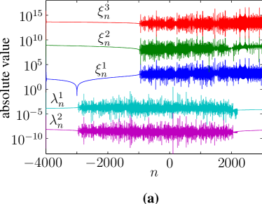
Figure 3: (Color online.) Panel (a) shows the absolute value of the coefficients from Eq. (27) and Eq. (28), used for the transformed recurrence relations (25) and (26). Here, a starting index of $M_{-}=-4000$ and initial values of $\xi_{M_{-}}^{1,2,3}=\lambda_{M_{-}}^{1,2}=1$ were used. Note that for better visibility, all curves except $\xi_{n}^{1}$ have been shifted vertically on the logarithmic ordinate axis by multiplication with a suitable constant ($10^{10}$ for $\xi_{n}^{3}$, $10^{5}$ for $\xi_{n}^{2}$, $10^{-7}$ for $\lambda_{n}^{1}$, and $10^{-12}$ for $\lambda_{n}^{2}$). In panel (b), we display the absolute values of $f_{n}$ and $g_{n}$, which result after completing step 3 in the algorithm described, i.e. before normalizing. The dash-dotted lines indicate the starting indices $M_{\pm}$, here $M_{-}=-3300$, and $M_{+}=2350$. The cutoff indices $n_{-}=-3000$, $n_{+}=2063$ are plotted with dashed lines. An example of a suitable “matching index” $K=0$ (see step 4 of the algorithm) is drawn by a solid line. The initial values used to calculate the curves were $f_{M_{+}}=10^{-20}/2$, $f_{M_{+}+1}=0$, $f_{M_{+}+2}=10^{-20}$, and $g_{M_{+}}=0$, $g_{M_{+}+1}=10^{17}$. Note that in panel (b), no vertical shifting was applied. The inset shows a magnification of the cutoff region for positive $n$, where the diverging behavior of $g_{n}$ for $n>n_{+}$ is clearly seen. In both graphs we have $x=y=10^{3}$, same as in Fig. 2.

To illustrate some of the intermediate steps of the algorithm, we show in Fig. 3 the typical behavior of the coefficients $\xi_{n}^{1,2,3}$ and $\lambda_{n}^{1,2}$ calculated in step 2, and also the result after step 3, before normalization of the arrays $f_{n}$ and $g_{n}$. Concluding the description of our recursive algorithm, we summarize the different integer indices which occur in the problem, which is useful to have in mind in the ensuing discussion: $n_{-}$ and $n_{+}$ are the negative and positive cutoff indices, respectively, and are fixed by the values of the arguments $x$ and $y$ through Eq. (24). $M_{-}$ and $M_{+}$ are the negative and positive starting indices, respectively. For the algorithm to converge, they should be chosen such that $M_{-}<n_{-}$, and $M_{+}>n_{+}$. The accuracy of the computed approximation to $J_{n}(x,y)$ will increase if the distances $n_{-}-M_{-}$, $M_{+}-n_{+}$ are increased (see Sec. IV). $K$ is a matching index, where the solutions $f_{n}$ and $g_{n}$ computed with different recurrence relations should be matched, and should satisfy $n_{-}<K<n_{+}$. Finally, $n_{\textrm{min}}$ and $n_{\textrm{max}}$ are the indices between which numerical values for $J_{n}(x,y)$ are sought. Except for the requirements $n_{\textrm{min}}>M_{-}$, $n_{\textrm{max}}<M_{+}$, and $n_{\textrm{min}}\leq n_{\textrm{max}}$, they can be arbitrarily chosen. The usual requirement is however $n_{\textrm{min}}\leq n_{-}$, $n_{\textrm{max}}\geq n_{+}$, which in that case implies the following inequality chain for the different indices involved:

$$M_{-}<n_{\textrm{min}}\leq n_{-}<K<n_{+}\leq n_{\textrm{max}}<M_{+}.$$ (32)

III.3 Demonstration of numerical stability

In this subsection we show, using arguments similar to those in Oliver (1968a), that the previously presented algorithm is numerically stable. Since the functions $J_{n}$, $Y_{n}$, $X_{n}$ and $Z_{n}$ (see Fig. 2) form a complete set of functions with respect to the recurrence relation (11), we can decompose any solution $y_{n}$ to the four-term recurrence relation (25) as

$$y_{n}=a_{1}\,J_{n}+a_{2}\,Y_{n}+a_{3}\,X_{n}+a_{4}\,Z_{n}.$$ (33)

The constants $a_{1}$, $a_{2}$, $a_{3}$, $a_{4}$ can be found from the initial conditions. For general $i$ in the range $N-2\leq i\leq N$, where $N$ is a general starting index (later we will take $N=M_{-}$), we have

$$y_{i}=a_{1}\,J_{i}+a_{2}\,Y_{i}+a_{3}\,X_{i}+a_{4}\,Z_{i},$$ (34)

but we can rewrite $y_{N+1}$ using the four-term recurrence in Eq. (25) as

$$\begin{split}&y_{N+1}=-\frac{1}{2y}\,\left(\xi^{1}_{N}\,y_{N}+\xi^{2}_{N}\,y_{N-1}+\xi^{3}_{N}\,y_{N-2}\right)\\[8.61108pt] &\quad=a_{1}\,J_{N+1}+a_{2}\,Y_{N+1}+a_{3}\,X_{N+1}+a_{4}\,Z_{N+1},\end{split}$$ (35)

for fixed starting integer $N$.

If we now for simplicity take the initial value at the upper boundary of the recursion $y_{N+1}=0$, by selecting the initial values $\xi^{1,2,3}_{N}$ for the coefficients accordingly, then we can choose (provided the system (35) is nonsingular, so that a solution exists) three sets of initial conditions $y^{t}_{i}$, $1\leq t\leq 3$, $N-2\leq i\leq N$, so that depending on which set is chosen, the constants $a_{j}$ in Eq. (33) are

$$a_{j}=\delta_{jt},\qquad 1\leq j\leq 3,\quad 1\leq t\leq 3,$$ (36)

where $\delta_{jt}$ is the Kronecker delta, leading to the solutions $y^{t}_{n}$ with $1\leq t\leq 3$. By requiring (36), we have implicitly reduced the solution to a linear combination of just two solutions, with nonvanishing components of one of $J_{n}$, $X_{n}$, $Y_{n}$ on the one hand, and $Z_{n}$ on the other hand. The remaining constant $a_{4}$ is obtained, for each set, from

$$y^{t}_{N+1}=0=\delta_{1t}J_{N+1}+\delta_{2t}Y_{N+1}+\delta_{3t}X_{N+1}+a_{4}Z_{N+1}\,,$$ (37)

assuming $Z_{N+1}\neq 0$. Because we have reduced the solutions $y^{t}_{n}$ to be linear combinations of just two functions, we immediately see that the three sets of initial values correspond to the three fundamental solutions $y_{n}^{1,2,3}$ to the four-term recurrence relation (25),

$$\begin{split}y^{1}_{n}&=J_{n}-\frac{J_{N+1}}{Z_{N+1}}Z_{n},\\ y^{2}_{n}&=Y_{n}-\frac{Y_{N+1}}{Z_{N+1}}Z_{n},\\ y^{3}_{n}&=X_{n}-\frac{X_{N+1}}{Z_{N+1}}Z_{n}.\end{split}$$ (38)

If now $N$ is taken small enough, $N=M_{-}<n_{-}$, by virtue of Eq. (19), the three fundamental solutions $y_{n}^{1,2,3}$ turn to the three functions $J_{n}$, $Y_{n}$, and $X_{n}$. We have basically eliminated the unwanted solution $Z_{n}$ by rewriting the five-term recurrence (11) into a four-term recurrence relation (25).

In other words, the reduced four-term recurrence relation (25), with the coefficients $\xi^{1,2,3}_{n}$ evaluated according to (27) in the direction of increasing $n$ from initial values $\xi^{1,2,3}_{M_{-}}$, $M_{-}<n_{-}$ with a safety margin, has to a very good approximation the three functions $J_{n}$, $Y_{n}$, and $X_{n}$ as fundamental solutions. This means that a solution $f_{n}$ to the recurrence relation (25), started with initial values $f_{l}$, $M_{+}\leq l\leq M_{+}+2$, $M_{+}>n_{+}$ with a safety margin, and applied in the direction of decreasing $n$ will be almost proportional to $J_{n}$ for $n<M_{+}$, by the same arguments as in subsection III.1, because after having eliminated $Z_{n}$, the wanted solution $J_{n}$ is the only one which is suppressed for $n\to\infty$. This is however only true down to the negative cutoff index $n_{-}$ below which an admixture of the other unwanted solution $Y_{n}$ takes over, see Fig. 3.

Similarly, for the three-term recurrence relation (26), we can write a generic solution $v_{n}$ in terms of the three fundamental solutions to the four-term recurrence relation (25),

$$v_{n}=b_{1}\,J_{n}+b_{2}\,X_{n}+b_{3}\,Y_{n}.$$ (39)

Again, there exist two sets $v^{s}_{j}$, $1\leq s\leq 2$, $N-1\leq j\leq N+1$, of initial conditions, with $v^{1,2}_{N+1}=0$, so that

$$b_{j}=\delta_{sj}.$$ (40)

The two fundamental solutions to Eq. (25) are therefore

$$\begin{split}v^{1}_{n}&=J_{n}-\frac{J_{N+1}}{Y_{N+1}}\,Y_{n},\\ v^{2}_{n}&=X_{n}-\frac{X_{N+1}}{Y_{N+1}}\,Y_{n}\,.\end{split}$$ (41)

Thus, provided the recurrence for the coefficients of the three-term recurrence given in Eq. (28) is started at sufficiently small, negative $N=M_{-}<n_{-}$, and applied in the forward direction, a solution $g_{n}$ to the three-term recurrence relation (26), started at a large $M_{+}>n_{+}$ and performed in the direction of decreasing $n$, will, to a good approximation, be proportional to $J_{n}$ for $n<n_{-}$. Combining the solution $f_{n}$ to the four-term equation (25) with the solution $g_{n}$ to the three-term equation (26) at the matching index $K$, where $n_{-}<K<n_{+}$ then yields a solution proportional to $J_{n}$ for all $n$, $n_{\textrm{min}}\leq n\leq n_{\textrm{max}}$. The proportionality constant is found using the sum rule (10).

Having settled the question of convergence, we comment briefly on how to numerically calculate the complementary solutions $Y_{n}$, $X_{n}$, and $Z_{n}$, shown in Fig. 2. We assume the most interesting case 1, $x<8y$. The function $X_{n}$ can be computed by using the original recurrence relation (11) in the direction of increasing $n$, starting at an index $N<-2y+x$, i.e. in region $b_{1}$. Here $X_{n}$ quickly outgrows the other solutions to leave only the “pure” $X_{n}$ after a few iterations. For $Z_{n}$, we similarly use the original recurrence relation (11), but this time in the direction of decreasing $n$, and starting at a large positive index $N>n_{+}$ [for the definition of $n_{+}$, see Eq. (24)]. However, in this region $J_{n}$ grows as fast as $Z_{n}$, and a solution $y_{n}$ calculated this way will be a linear combination $y_{n}=a_{1}\,J_{n}+a_{2}\,Z_{n}$ for $n>-2y+x$, the constants $a_{1,2}$ depending on the initial values. For $n<-2y+x$ (in region $b_{1}$), $Z_{n}$ grows faster with decreasing $n$ than the other fundamental solutions, so that here $y_{n}=a_{2}\,Z_{n}$. Finally, using the four-term relation (25) in the backward direction, starting at index $N<n_{+}$ in region $c_{1}$, yields a solution $x_{n}=a_{1}J_{n}+a_{2}Y_{n}+a_{3}X_{n}$ for $-2y+x<n<n_{+}$, $x_{n}=a_{1}J_{n}+a_{2}Y_{n}$ for $n_{-}<n<-2y+x$ and $x_{n}=a_{2}Y_{n}$ for $n<n_{-}$.

IV Discussion

IV.1 Accuracy

It is necessary to investigate how the accuracy of the computed approximation $h_{n}$ depends on the starting indices $M_{-}$, $M_{+}$. To this end, we define the positive “safety margin” parameter $\Delta$ through

$$M_{-}=n_{\textrm{min}}-\Delta,\qquad M_{+}=n_{\textrm{max}}+\Delta,$$ (42)

so that specifying $\Delta$ fixes both the upper and the lower starting index, and we also define the relative error

$$\epsilon_{\textrm{rel}}=\left\lvert\frac{h_{n}-J_{n}(x,y)}{J_{n}(x,y)}\right\rvert.$$ (43)

In Fig. 4, we show the relative accuracy that can be obtained by the method presented in this paper, as a function of $\Delta$, for different values of the arguments $x$ and $y$, and different index $n$ in the obtained array $h_{n}$. We have numerically verified that a performance, similar to the one presented in Fig. 4, can be expected even close to zeros of $J_{n}(x,y)$ (that is, for a general index $n$, $n_{\textrm{min}}\leq n\leq n_{\textrm{max}}$, where $J_{n}(x,y)=0$ or $J_{n}(x,y)\approx 0$), although in this case the estimates remain valid only for the absolute instead of the relative error. Specifically, in the panels (a)–(c) of Fig. 4, we evaluate the relative error $\epsilon_{\textrm{rel}}$ at $n=0$ and take $n_{\textrm{min}}=n_{-}$, $n_{\textrm{max}}=n_{+}$ [see Eq. (24), and also the discussion preceding Eq. (32)], which means that the recurrence is started at a distance $\Delta$ from the cutoff indices. The different curves in the graphs correspond to the following values of $x$ and $y$: In (a), we have $2y=x=10$ for curve 1 (blue line), $2y=x=10^{2}$ for curve 2 (green line), and $2y=x=10^{3}$ for curve 3 (red line). For these values of $x$, $y$, the index $n=0$ corresponds to the border between the two saddle point regions $b_{1}$ and $c_{1}$. We note that $J_{n}(x,y)$ cannot be accurately evaluated in such border regions using the simple saddle point approximation Leubner (1981); Korsch et al. (2006), but that our method works well here. In (b) we have $y=10x=10$ for curve 1 (blue line), $y=10^{2}x=10^{2}$ for curve 2 (green line), and $y=10^{3}x=10^{3}$ for curve 3 (red line), demonstrating the method for cases where the ratio $y/x$ is large. In (c), we have instead a small ratio $y/x$: $x=10y=10$ for curve 1 (blue line), $x=10^{2}y=10^{2}$ for curve 2 (green line), and $x=10^{3}y=10^{3}$ for curve 3 (red line). Finally, in (d) we show the case where $J_{n}(x,y)$ is evaluated in the cutoff region, where for all three curves $|J_{n}(x,y)|$ is of order $10^{-10}$. Here, we have $y=x=10$, $n=n_{\textrm{max}}=55$, $n_{\textrm{min}}=n_{-}-n+n_{+}=-64$ for curve 1 (blue line), $y=x=10^{2}$, $n=n_{\textrm{max}}=270$, $n_{\textrm{min}}=n_{-}-n+n_{+}=-364$ for curve 2 (green line), and $y=x=10^{3}$, $n=n_{\textrm{max}}=2200$, $n_{\textrm{min}}=n_{-}-n+n_{+}=-3137$ for curve 3 (red line). The value $n_{\textrm{min}}$ has in all cases in graph (d) been chosen so that the distance $n_{-}-n_{\textrm{min}}$ equals $n_{\textrm{max}}-n_{+}$. Recall that the starting indices $M_{\pm}$ follows by fixing $n_{\textrm{min}}$, $n_{\textrm{max}}$, and $\Delta$, by Eq. (42). The black circles in the graphs (a)–(d) have been obtained from Eq. (45), using approximation (46). For the calculations, computer arithmetic with 32 decimals was used.

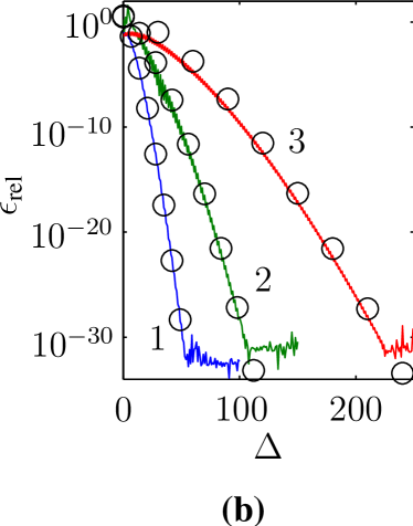
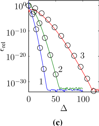
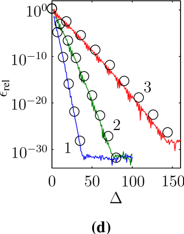
Figure 4: (Color online.) The relative error $\epsilon_{\textrm{rel}}$, as defined in Eq. (43), as a function of the “safety margin” parameter $\Delta$ [see Eq. (42)]. In each of the different parameter ranges considered, an exponential decrease of the obtained error with the safety margin parameter is observed, demonstrating the applicability of the recursive method. In (a), we consider parameters such that $x=2y$, in (b) we have large ratio $y/x$, in (c) small ratio $y/x$, and in (d) results for the cutoff region are presented. Detailed explanation of the parameter regions considered is in the text. In all graphs, black circles represent the approximation for the relative error obtained from Eqs. (45) and (46).

An analytic formula for the relative error can be obtained by assuming that after normalization, the calculated value $h_{n}$ is of the form (writing out the dependence of $Y_{n}$ on the arguments $x$ and $y$ explicitly),

$$h_{n}=J_{n}(x,y)-\frac{J_{M_{-}}(x,y)}{Y_{M_{-}}(x,y)}\,Y_{n}(x,y),$$ (44)

for starting index $M_{-}<n_{-}$, similarly to the case for the ordinary Bessel function [see Eq. (22)]. This is a simplified assumption, since the total error in general is more complicated, but Eq. (44) can nevertheless be used to make practical predictions about the dependence of $\epsilon_{\textrm{rel}}$ on $\Delta$. Equation (44) yields for the approximative relative error

$$\epsilon_{\textrm{rel, app}}=\left\lvert\frac{h_{n}-J_{n}(x,y)}{J_{n}(x,y)}\right\rvert=\left\lvert\frac{J_{M_{-}}(x,y)}{Y_{M_{-}}(x,y)}\,\frac{Y_{n}(x,y)}{J_{n}(x,y)}\right\rvert.$$ (45)

An approximation for the amplitude of $Y_{M_{-}}(x,y)$ for $M_{-}<n_{-}$ can be obtained from the saddle point expression (14) for $J_{n}(x,y)$, but reversing the sign of the real part of the argument of the exponential. If we write the saddle point approximation of $Y_{n}(x,y)$ as $Y_{n}(x,y)=G_{+}(n)+G_{-}(n)$, we have

$$\begin{split}&\left\lvert\frac{J_{M_{-}}(x,y)}{Y_{M_{-}}(x,y)}\right\rvert\approx\left\lvert\frac{F_{+}(M_{-})+F_{-}(M_{-})}{G_{+}(M_{-})+G_{-}(M_{-})}\right\rvert\approx\left\lvert J_{M_{-}}(x,y)\right\rvert^{2}\\ &\quad\approx\left(\mathrm{e}^{-\left|\mathrm{Re}[\mathrm{i}f(\theta_{+})-\mathrm{i}M_{-}\theta_{+}]\right|}+\mathrm{e}^{-\left|\mathrm{Re}[\mathrm{i}f(\theta_{-})-\mathrm{i}\,M_{-}\theta_{-}]\right|}\right)^{2},\end{split}$$ (46)

where $f(\theta)$ is defined as after Eq. (14), and $\theta_{\pm}$ denote the two different saddle point solutions from Eq. (12), with $n=M_{-}$. The last approximation in Eq. (46) neglects the preexponential factor and the oscillating factor in the saddle point approximation (14), which is sufficient for an order-of-magnitude estimate. The ratio ${Y_{n}(x,y)}/{J_{n}(x,y)}$ in (45) can be approximated with unity for $n$ in the oscillating region [graph (a), (b), and (c) in Fig. 4], and with the simplified saddle point approximation (46) for $n$ in the cutoff region [graph (d) in Fig. 4]. The approximation (45) together with (46) for the relative error is plotted as circles in Fig. 4. Clearly the approximate formula can be used for practical estimates of how far out the recurrence should be started if a specific accuracy is sought for the array of generalized Bessel functions to be computed. Formula (46) also explains the exponential decrease in relative error observed in Fig. 4.

IV.2 Comparison with other methods

Here we briefly comment on the performance of the presented algorithm as compared to other ways of numerically evaluating the generalized Bessel function. Let us compare to an alternative algorithm based on the evaluation of ordinary Bessel functions using the techniques outlined in Sec. III.1, where we first calculate two arrays $J_{2s+n}(x)$, $J_{s}(y)$ of ordinary Bessel functions by Miller’s algorithm and later calculate the generalized Bessel functions using Eq. (9). Calculation of the arrays of ordinary Bessel functions then requires two recurrence runs, and to obtain the numerical value $J_{n}(x,y)$, in addition the sum $\sum_{s=-\infty}^{\infty}J_{2s+n}(x)J_{s}(y)$ has to be performed. This means that since the generalized Miller’s algorithm requires two recurrence runs only, for calculation of a single value $J_{n_{0}}(x,y)$, the two methods demand a comparable amount of time. However, the calculation of a single generalized Bessel function is not the aim of our considerations: for the whole array $J_{n}(x,y)$, $n_{\textrm{min}}\leq n\leq n_{\textrm{max}}$, the reduction in computer time due to the elimination of the calculation of the sums $\sum_{s=-\infty}^{\infty}J_{2s+n}(x)J_{s}(y)$ leads to an order-of-magnitude gain with respect to computational resources while the accuracy obtained by the two different methods is similar.

The second method with which to compare is the asymptotic expansion by integration through the saddle points, as presented in Leubner (1981). For evaluation of a single value $J_{n_{0}}(x,y)$, with moderate accuracy demands, the saddle-point integration is of course the best method, especially for large values of the parameters $n$, $x$ and $y$. The drawback of this method is the relatively complex implementation Leubner (1981), and in addition, an increase in the accuracy of a saddle-point method typically is a nontrivial task which involves higher-order expansions of the integrand about the saddle point, and this typically leads to very complicated analytic expressions for higher orders, especially for an integrand with a nontrivial structure as in Eq. (1). See however Huybrechs and Vandewalle (2006) for a possibly simpler numerical method, the “numerical steepest descent method”. In any case, if the complete array $J_{n}(x,y)$, $n_{\textrm{min}}\leq n\leq n_{\textrm{max}}$ is sought to high accuracy, as it is the case for second-order laser-related problems, then our method is necessarily better, since the time spent on one recursive step is very brief.

V Illustrative Considerations for the Dirac–Volkov Solutions

In this Section, we consider the Volkov solution, the analytic solution to the Dirac (or Klein-Gordon) equation coupled to an external, plane-wave laser field. We show that the generalized Bessel functions can be directly interpreted as the amplitudes for discrete energy levels of a quantum laser-dressed electron, corresponding to the absorption or emission of a specific number of laser photons.

V.1 Physical origin of the recurrence relation

There is a direct, physical way to derive the recurrence relation satisfied by the generalized Bessel function, in the context of relativistic laser-matter interactions. The result of this approach defines $J_{n}(x,y)$ in terms of the recurrence relation and a normalization condition, even on the level of spinless particles, i.e. on the level of Klein-Gordon theory. In this section, we set $\hbar=c=1$, denote the electron’s charge and mass by $e=-|e|$ and $m$, respectively, and write dot products between relativistic four-vectors as $u\cdot v=u_{\mu}v^{\mu}=u^{0}v^{0}-\vec{u}\cdot\vec{v}$, for two four-vectors $u^{\mu}$ and $v^{\mu}$. The space-time coordinate is denoted by $z^{\mu}=(t,\vec{x})$, in order not to cause confusion with the argument $x$ of $J_{n}(x,y)$, and $k\cdot z=\omega\,t-\vec{k}\cdot\vec{x}$ is the phase of the laser field. The $4\times 4$ Dirac gamma matrices are written as $\gamma^{\mu}$.

Let us consider the Klein-Gordon equation $\left[\left(\mathrm{i}\partial_{z}-eA\right)^{2}-m^{2}\right]\psi(z)=0$ for the interaction of a spinless particle of charge $e$ with an external laser field of linear polarization $A^{\mu}(z)=a^{\mu}\cos(k\cdot z)$,

$$\begin{split}\ &\bigg{[}-\partial^{2}_{z}-2\mathrm{i}e\cos(k\cdot z)\,a\cdot\partial_{z}\\ &\quad+\frac{e^{2}\,a^{2}}{2}\cos(2k\cdot z)-m^{2}-\frac{|e^{2}a^{2}|}{2}\bigg{]}\psi(z)=0\,.\end{split}$$ (47)

Here $a^{\mu}=(0,\vec{a})$ is the polarization vector, and $k^{\mu}=(\omega,\vec{k})$ is the propagation wave vector of the laser field, with $k\cdot k=k\cdot a=0$. We also introduce the four-vector $q^{\mu}$, the so-called effective momentum Berestetskii et al. (1982), which fulfills

$$q^{2}=m^{2}+{\textstyle{\frac{1}{2}}}\,|e^{2}a^{2}|\,.$$ (48)

We now insert the Floquet ansatz Chu and Telnov (2004) for the wave function

$$\psi(z)=\mathrm{e}^{-\mathrm{i}q\cdot z}\sum_{s}B_{s}\,\mathrm{e}^{-\mathrm{i}sk\cdot z}\,,$$ (49)

where the coefficients $B_{n}$ are independent of $z^{\mu}$, into Eq. (LABEL:Klein-Gordon_Floquet_ansatz). From this representation, we see that the factor $\mathrm{e}^{-\mathrm{i}sk\cdot z}$, actually has the same form as a phase factor characterizing the absorption of $s$ laser photons from the laser field, as we integrate over the Minkowski coordinate $z$ in the calculation of an $S$-matrix element. For negative $s$, we instead have emission into the laser mode. Equation (49) also leads to a relation for the coefficients $B_{s}$,

$$\begin{split}&\sum_{s=-\infty}^{\infty}\left[x\cos(\phi)-2y\cos(2\phi)-s\right]\,B_{s}\,\mathrm{e}^{-\mathrm{i}s\phi}=0\,,\\ &x=\frac{e\,a\cdot q}{k\cdot q}\,,\qquad y=\frac{e^{2}\,a^{2}}{8k\cdot q}\,,\qquad\phi=k\cdot z\,.\end{split}$$ (50)

Multiplying Eq. (LABEL:a_relation_for_the_coefficients_A_s) with $\mathrm{e}^{\mathrm{i}n\phi}$, and integrating over one period, we obtain the recurrence relation (11), if we identify

$$B_{n}\equiv J_{n}(x,y)\,.$$ (51)

For the wave function (49) constructed from the solution to the recurrence relation (11) to be finite, we must demand $J_{n}(x,y)$ to be normalizable. This is expressed by the condition (10). Furthermore, using the property (2) of $J_{n}(x,y)$, we can perform the sum over $s$ in (49), with the result

$$\psi(z)=\mathrm{e}^{-\mathrm{i}q\cdot z-\mathrm{i}x\sin\phi+\mathrm{i}y\sin(2\phi)},$$ (52)

which is the form in which the Volkov solution is usually presented Berestetskii et al. (1982).

For comparison, the solution $\Psi(z)$ to the Dirac equation in presence of a linearly polarized laser field,

$$\left(\mathrm{i}\,\gamma\cdot\partial_{z}-e\,a\cdot\gamma\,\cos\phi-m\right)\,\Psi(z)=0$$ (53)

reads

$$\begin{split}\Psi(z)=\mathrm{e}^{-\mathrm{i}q\cdot z}\sum_{s=-\infty}^{\infty}\Big{(}&\frac{ek\cdot\gamma\,a\cdot\gamma}{4\,k\cdot q}\,[J_{s+1}(x,y)+J_{s-1}(x,y)]\\ &+J_{s}(x,y)\Big{)}\,\mathrm{e}^{-\mathrm{i}\,s\,\phi}\,u_{q}\,,\end{split}$$ (54)

where $x$, $y$ are defined in Eq. (LABEL:a_relation_for_the_coefficients_A_s), and $u_{q}$ is a Dirac bispinor satisfying

$$\left(\gamma\cdot q+2\,y\,\gamma\cdot k-m\right)\,u_{q}=0\,.$$ (55)

The four-vector $p^{\mu}=q^{\mu}+2yk^{\mu}$ can be identified as the asymptotic momentum of the particle, or the residual momentum as the laser field is turned off.

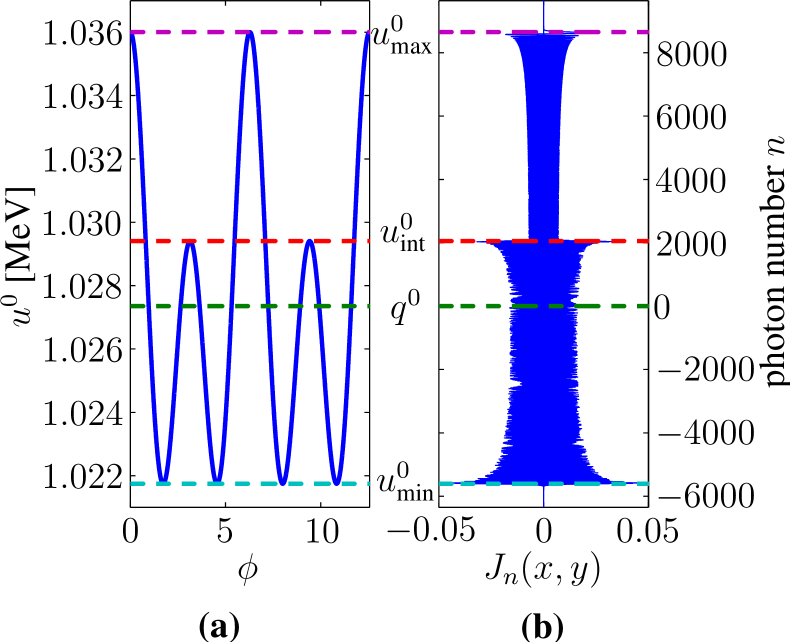
Figure 5: (Color online.) Illustration of the classical-quantum correspondence of a laser-dressed electron. Shown to the left [panel (a)] with a solid blue line is the classical energy $u^{0}$ [see Eq. (57)] as a function of the phase $\phi$, for $\omega=1$ eV, laser intensity $I=10^{16}$ W/cm² (corresponding to $|e\,a|/m=0.1$ where $a$ is the laser polarization four-vector), initial energy $p^{0}=2m$, and initial angle $\theta=0.54^{\circ}$, with $\vec{p}\cdot\vec{k}=|\vec{p}|\,\omega\cos\theta$. These parameters give $x=3.3\times 10^{3}$, and $y=-2.7\times 10^{3}$ for the arguments of $J_{n}(x,y)$. The dashed lines show the minimum classical energy $u^{0}_{\textrm{min}}$, the maximum classical energy $u^{0}_{\textrm{max}}$, the average energy $q^{0}$, and the intermediate energy level (local maximum) $u^{0}_{\textrm{int}}$, as indicated in the center of the figure. In panel (b), we display the quantum mechanical amplitude $J_{n}(x,y)$ of energy level $n$, which has energy $q^{0}+n\omega$ [see Eq. (49)]. Here positive index $n$ corresponds to absorbing $n$ number of photons from the laser field, while negative $n$ means emitting $|n|$ number of photons into the laser mode. The graph is arranged such that $n=0$ corresponds to the average energy $q^{0}$. The cutoff indices are nicely reproduced by the classical maxima and minima.

V.2 Classical-quantum correspondence of Volkov states

It follows from the expression (49), that a quantum Volkov state (we consider the spinless case for simplicity) can be regarded as a superposition of an infinite number of plane waves with definite, discrete, four-momenta $q^{\mu}+nk^{\mu}$. The amplitude to find the particle with four-momentum $q^{\mu}+nk^{\mu}$ is given by $J_{n}(x,y)$, with $x$ and $y$ as in Eq. (LABEL:a_relation_for_the_coefficients_A_s). Therefore, it might seem that the particle can acquire arbitrarily high energy in the field. That this is not so, follows from the exponential decay of $J_{n}(x,y)$ beyond the cutoff indices, as discussed in subsection II.2. In the following, we show that the cutoff indices can also be derived as the lowest and highest energy of a classical particle moving in a laser field. To this end, we first recall the classical, relativistic equations of motion of a particle of charge $e$ and mass $m$, moving in the laser potential $A^{\mu}=a^{\mu}\cos\phi$:

$$\frac{\mathrm{d}u^{\mu}}{\mathrm{d}\tau}=\frac{e}{m}(a^{\mu}\,k\cdot u-k^{\mu}\,a\cdot u)\sin\phi,$$ (56)

where $u^{\mu}$ is the kinetic momentum, and $\tau$ is the proper time. The solution reads Sarachik and Schappert (1970); Meyer (1971), assuming initial phase $\phi_{0}=\pi/2$,

$$u^{\mu}=p^{\mu}+x\,k^{\mu}\,\cos\phi-4\,y\,k^{\mu}\,\cos^{2}\phi-e\,a^{\mu}\,\cos\phi\,,$$ (57)

where $p^{\mu}$ is the asymptotic momentum. Note that as $u^{\mu}$ is the physical momentum, it is gauge invariant under $A^{\mu}\to A^{\mu}+\Lambda k^{\mu}$, where $\Lambda$ is an arbitrary function. The phase average is exactly the effective momentum, $\overline{u^{\mu}}=p^{\mu}-k^{\mu}e^{2}a^{2}/(4k\cdot p)=q^{\mu}$. In Fig. 5, we consider the energy $u^{0}$ as a function of the phase $\phi$ and compare it with the discrete energy levels $q^{0}+n\,\omega$ of the quantum wave function. We see that the maximal and minimal energy of the classical particle correspond exactly to the cutoff indices of the generalized Bessel function. The probability for the quantum particle to have an energy larger (or smaller) than the classically allowed energy is thus exponentially small. Interestingly, the local maxima of the classical energy $u^{0}$, labeled $u^{0}_{\textrm{int}}$ in Fig. 5, coincide with the transition between the two different saddle point regions of $J_{n}(x,y)$.

VI Conclusions

We have presented a recursive algorithm for numerical evaluation of the generalized Bessel function $J_{n}(x,y)$, which is important for laser-physics related problems, where the evaluation of large arrays of generalized Bessel functions is crucial. In general, we can say that the laser parameters fix the arguments $x$ and $y$ of the generalized Bessel function $J_{n}(x,y)$, while the index $n$ characterizes the number of exchanged laser photons.

As evident from Figs. 1 and 2, complementary solutions $Y_{n}$, $X_{n}$, and $Z_{n}$ to the recurrence relation (11) satisfied by $J_{n}(x,y)$ are central to our algorithm. By removing the sources of numerical instability, which are the exponentially growing complementary solutions, in a first recurrence run, we are able to construct a stable recursive algorithm, similar to Miller’s algorithm for the ordinary Bessel function, but suitably enhanced for the generalized Bessel function. Numerical stability is demonstrated, and the obtainable accuracy is studied numerically and by an approximate formula (see Sec. IV). The algorithm is useful especially when a large number of generalized Bessel function of different index, but of the same argument, is to be generated. As is evident from the discussion in Sec. V, a fast and accurate calculation of generalized Bessel functions leads to a quantitative understanding of the quantum-classical correspondence for a laser-dressed electron.

VII Acknowledgment

U.D.J. acknowledges support by the Deutsche Forschungsgemeinschaft (Heisenberg program) during early stages of this work.

*

Appendix A Integral representation of the complementary solutions

In this Appendix, we present the expressions for the integral representations of the complementary solutions $Y_{n}(x,y)$, $Z_{n}(x,y)$, and $X_{n}(x,y)$ to the recurrence relation (11), without giving any details about the mathematical considerations which lead to these representations. The integrals read

$$Y_{n}(x,y)= -\frac{1}{\pi}\int_{0}^{\infty}[\cos(n\pi/2-x\cosh\theta)\mathrm{e}^{n\theta}$$

$$\quad\qquad\quad+(-1)^{n}\mathrm{e}^{-n\theta-x\sinh\theta}]\mathrm{e}^{-y\sinh 2\theta}\mathrm{d}\theta$$

$$\quad-\frac{1}{\pi}\int_{\pi/2}^{\pi}\sin({n\theta-x\sin\theta+y\sin 2\theta})\mathrm{d}\theta,$$ (58)

$$X_{n}(x,y)= -\frac{1}{\pi}\int_{0}^{\infty}\sin(n\pi/2-x\cosh\theta)\,\mathrm{e}^{n\theta-y\sinh 2\theta}\mathrm{d}\theta$$

$$\quad-\frac{1}{\pi}\int_{0}^{\pi/2}\cos({n\theta-x\sin\theta+y\sin 2\theta})\mathrm{d}\theta,$$ (59)

$$Z_{n}(x,y)= \;-\frac{1}{\pi}\int_{0}^{\pi}\sin({n\theta-x\sin\theta+y\sin 2\theta})\mathrm{d}\theta$$

$$\quad-\frac{1}{\pi}\int_{0}^{\infty}[(-1)^{n}\mathrm{e}^{-x\sinh\theta}-\mathrm{e}^{x\sinh\theta}]$$

$$\qquad\qquad\quad\times\mathrm{e}^{-n\theta-y\sinh 2\theta}\mathrm{d}\theta.$$ (60)

Recall that we consider non-zero, positive values of the arguments $x$ and $y$, and an arbitrary integer $n$. By partial integration, the functions (A)—(A) verify the recurrence relation (11). The prefactor has been selected for each case so that the functions $X_{n}(x,y)$, $Y_{n}(x,y)$, and $Z_{n}(x,y)$ have the same amplitude as $J_{n}(x,y)$ in the oscillating region, and this choice also implies that the functions $Y_{n}(x\to 0,y)$ and $Z_{n}(x\to 0,y)$, for even and odd $n$, respectively, can be expressed as Neumann functions of fractional order. (The latter statement is also given here without proof.) A more detailed discussion of the mathematical properties of the four functions defined by the integral representations (1), (A), (A) and (A) will be given elsewhere. For all considerations reported in the current article, the detailed knowledge of the integral representations is not necessary; it is sufficient to know the recurrence relation (11) that they fulfill.

References

- (1)
- Volkov (1935) D. M. Volkov, Z. Phys. 94, 250 (1935).
- Reiss (1962) H. R. Reiss, J. Math. Phys. 3, 59 (1962).
- Nikishov and Ritus (1964) A. I. Nikishov and V. I. Ritus, Zh. Éksp. Teor. Fiz. 46, 776 (1964) [Sov. Phys. JETP 19, 529 (1964)].
- Brown and Kibble (1964) L. S. Brown and T. W. B. Kibble, Phys. Rev. 133, A705 (1964).
- Mittleman (1987) M. H. Mittleman, Phys. Rev. A 35, 4624 (1987).
- Müller et al. (2004) C. Müller, A. B. Voitkiv, and N. Grün, Phys. Rev. A 70, 023412 (2004).
- Sieczka et al. (2006) P. Sieczka, K. Krajewska, J. Z. Kamiński, P. Panek, and F. Ehlotzky, Phys. Rev. A 73, 053409 (2006).
- Lötstedt et al. (2007) E. Lötstedt, U. D. Jentschura, and C. H. Keitel, Phys. Rev. Lett. 98, 043002 (2007).
- Schnez et al. (2007) S. Schnez, E. Lötstedt, U. D. Jentschura, and C. H. Keitel, Phys. Rev. A 75, 053412 (2007).
- Roshchupkin (1985) S. P. Roshchupkin, Yad. Fiz. 41, 1244 (1985) [Sov. J. Nucl. Phys. 41, 796 (1985)].
- Müller et al. (2008) C. Müller, K. Z. Hatsagortsyan, and C. H. Keitel, Phys. Lett. B 659, 209 (2008).
- Müller et al. (2008) C. Müller, K. Z. Hatsagortsyan, and C. H. Keitel, Phys. Rev. A 78, 033408 (2008).
- Dattoli and Voykov (1993) G. Dattoli and G. Voykov, Phys. Rev. E 48, 3030 (1993).
- Sarachik and Schappert (1970) E. S. Sarachik and G. T. Schappert, Phys. Rev. D 1, 2738 (1970).
- Panek et al. (2002a) P. Panek, J. Z. Kamiński, and F. Ehlotzky, Phys. Rev. A 65, 033408 (2002a).
- Panek et al. (2002b) P. Panek, J. Z. Kamiński, and F. Ehlotzky, Phys. Rev. A 65, 022712 (2002b).
- Roman et al. (2000) J. S. Roman, L. Roso, and H. R. Reiss, J. Phys. B 33, 1869 (2000).
- Roman et al. (2003) J. S. Roman, L. Roso, and L. Plaja, J. Phys. B 36, 2253 (2003).
- Reiss (1980) H. R. Reiss, Phys. Rev. A 22, 1786 (1980).
- Reiss and Krainov (2003) H. R. Reiss and V. P. Krainov, J. Phys. A 36, 5575 (2003).
- Vanne and Saenz (2007) Y. V. Vanne and A. Saenz, Phys. Rev. A 75, 063403 (2007).
- Guo et al. (2008) L. Guo, J. Chen, J. Liu, and Y. Q. Gu, Phys. Rev. A 77, 033413 (2008).
- Gao et al. (1998) J. Gao, F. Shen, and J. G. Eden, Phys. Rev. Lett. 81, 1833 (1998).
- Gao et al. (2000) L. Gao, X. Li, P. Fu, R. R. Freeman, and D.-S. Guo, Phys. Rev. A 61, 063407 (2000).
- Dattoli et al. (1990) G. Dattoli, L. Giannessi, L. Mezi, and A. Torre, Nuovo Cim. 105 B, 327 (1990).
- Dattoli et al. (1991) G. Dattoli, A. Torre, S. Lorenzutta, G. Maino, and C. Chiccoli, Nuovo Cim. 106 B, 21 (1991).
- Dattoli et al. (1993) G. Dattoli, C. Chiccoli, S. Lorenzutta, G. Maino, M. Richetta, and A. Torre, J. Sci. Comp. 8, 69 (1993).
- Dattoli et al. (1995) G. Dattoli, G. Maino, C. Chiccoli, S. Lorenzutta, and A. Torre, Comput. Math. Appl. 30, 113 (1995).
- Dattoli et al. (1998) G. Dattoli, A. Torre, S. Lorenzutta, and G. Maino, Comput. Math. Appl. 35, 117 (1998).
- Korsch et al. (2006) H. J. Korsch, A. Klumpp, and D. Witthaut, J. Phys. A 39, 14947 (2006).
- Klumpp et al. (2007) A. Klumpp, D. Witthaut, and H. J. Korsch, J. Phys. A 40, 2299 (2007).
- Leubner (1981) C. Leubner, Phys. Rev. A 23, 2877 (1981).
- Lötstedt et al. (2009) E. Lötstedt, U. D. Jentschura, and C. H. Keitel, New J. Phys. 11, 013054 (2009).
- Bickley et al. (1960) W. G. Bickley, L. J. Comrie, J. C. P. Miller, D. H. Sadler, and A. J. Thompson, Bessel functions, Part II, functions of positive integer order, vol. X of Mathematical tables (Cambridge University Press, Cambridge, 1960).
- Gautschi (1967) W. Gautschi, SIAM Rev. 9, 24 (1967).
- Oliver (1968a) J. Oliver, Numer. Math. 11, 349 (1968a).
- Mattheij (1980) R. M. M. Mattheij, Numer. Math. 35, 421 (1980).
- Mattheij (1982) R. M. M. Mattheij, BIT 22, 79 (1982).
- Wimp (1984) J. Wimp, Computation with recurrence relations (Pitman Advanced Publishing Program, Boston, London, Melbourne, 1984), 1st ed.
- Olver (1997) F. W. J. Olver, Asymptotics and special functions (A K Peters, Natick, Massachusetts, 1997), A K Peters ed.
- Jordan (1960) C. Jordan, Calculus of finite differences (Chelsea Publishing Company, New York, 1960), 2nd ed.
- Mohr (1974) P. J. Mohr, Ann. Phys. 88, 52 (1974).
- Watson (1962) G. N. Watson, A treatise on the theory of Bessel functions (Cambridge University Press, Cambridge, 1962), 2nd ed.
- Matviyenko (1993) G. Matviyenko, Appl. Comput. Harmon. Anal. 1, 116 (1993).
- Olver (1964) F. W. J. Olver, Math. Comp. 18, 65 (1964).
- Oliver (1967) J. Oliver, Numer. Math. 9, 323 (1967).
- Olver and Sookne (1972) F. W. J. Olver and D. J. Sookne, Math. Comp. 26, 941 (1972).
- Ratis and Fernández de Córdoba (1993) Yu. L. Ratis and P. Fernández de Córdoba, Comput. Phys. Commun. 76, 381 (1993).
- du Toit (1993) C. F. du Toit, Comput. Phys. Commun. 78, 181 (1993).
- Yousif and Melka (1997) H. A. Yousif and R. Melka, Comput. Phys. Commun. 106, 199 (1997).
- Oliver (1968b) J. Oliver, Numer. Math. 12, 459 (1968b).
- Huybrechs and Vandewalle (2006) D. Huybrechs and S. Vandewalle, SIAM J. Numer. Anal. 44, 1026 (2006).
- Berestetskii et al. (1982) V. B. Berestetskii, E. M. Lifshitz, and L. P. Pitaevskii, Quantum Electrodynamics, vol. 4 (Elsevier, Oxford, 1982), 2nd ed.
- Chu and Telnov (2004) S.-I. Chu and D. A. Telnov, Phys. Rep. 390, 1 (2004).
- Meyer (1971) J. W. Meyer, Phys. Rev. D 3, 621 (1971).