The spatial distribution of stars in open clusters

Abstract

The analysis of the distribution of stars in open clusters may yield important information on the star formation process and early dynamical evolution of stellar clusters. Here we address this issue by systematically characterizing the internal spatial structure of 16 open clusters in the Milky Way spanning a wide range of ages. Cluster stars have been selected from a membership probability analysis based on a non-parametric method that uses both positions and proper motions and does not make any a priori assumption on the underlying distributions. The internal structure is then characterized by means of the minimum spanning tree method ($Q$ parameter), King profile fitting, and the correlation dimension ($D_{c}$) for those clusters with fractal patterns. On average, clusters with fractal-like structure are younger than those exhibiting radial star density profiles and an apparent trend between $Q$ and age is observed in agreement with previous ideas about the dynamical evolution of the internal spatial structure of stellar clusters. However, some new results are obtained from a more detailed analysis: (a) a clear correlation between $Q$ and the concentration parameter of the King model for those cluster with radial density profiles, (b) the presence of spatial substructure in clusters as old as $\sim 100$ Myr, and (c) a significant correlation between fractal dimension and age for those clusters with internal substructure. Moreover, the lowest fractal dimensions seem to be considerably smaller than the average value measured in galactic molecular cloud complexes.

1 Introduction

It is known that most stars are born within giant molecular clouds forming clusters (Lada & Lada, 2003). Numerical simulations demonstrate that star formation occurs mainly along the patterns defined by the densest regions of the molecular clouds (Bonnell et al., 2003). Thus, the hierarchical structure observed in some open clusters (see, for example, Larson, 1995) is presumably a consequence of its formation in a medium with an underlying fractal structure. This fractality is considered to be a clear signature of its own turbulent nature (Elmegreen & Scalo, 2004). Otherwise, open clusters having central star concentrations with radial star density profiles likely reflect the dominant role of gravity, either on the primordial gas structure or as a result of a rapid evolution from a more structured state (Lada & Lada, 2003).

It is therefore important to study the distribution of stars because it may yield some information on the formation process and early evolution of open clusters. It is necessary, however, that this kind of analysis is done by measuring the cluster structure in an objective, quantitative, as well as systematic way. The application of the two-point correlation function by Larson (1995) to young stars in Taurus suggested that the distribution of stars on spatial scales larger than the binary regime exhibits a fractal pattern with a projected dimension of $D\sim 1.4$. This value is very similar to the average value $D\sim 1.5\pm 0.2$ found by Simon (1997) for the Taurus, Ophiuchus, and Orion trapezium regions. More recent works find significantly smaller values for stars in Taurus, such as $D=1.02\pm 0.04$ (Hartmann, 2002) and $D=1.049\pm 0.007$ (Kraus & Hillenbrand, 2008). The difference could be at least partly due to differences in the completeness of the sample (Sánchez & Alfaro, 2008). Nakajima et al. (1998) studied the clustering of stars in the Orion, Ophiuchus, Chamaeleon, Vela, and Lupus regions obtaining significant variations from region to region in the range $1.2<D<1.9$. The interpretation of these results requires some caution because it has been shown that a good power-law fit to the two-point correlation function does not necessarily mean that the stellar distribution is fractal (Bate et al., 1998).

Cartwright & Whitworth (2004) developed a different method to quantify the structure of star clusters. Their method is based on the construction of the minimum spanning tree (MST) of the cluster and it has the important advantage of being able to distinguish between centrally concentrated and fractal-like structures. They concluded that the fractal dimension of the three-dimensional distribution of stars in Chamaeleon and IC 2391 is $D_{f}=2.25\pm 0.25$, whereas in Taurus $D_{f}=1.9\pm 0.2$ (see also Schmeja & Klessen, 2006). These dimensions seem too small when compared with the average value of $D_{f}\simeq 2.6-2.7$ suggested for the structure of the interstellar medium (Sánchez et al., 2005, 2007b), although higher dimension values have been reported using this technique (MST) on clusters in other regions such as Serpens and Ophiuchus (Schmeja et al., 2008). The rapid early evolution of star clusters may complicate the picture, because the parameters characterizing the cluster structure must only be taken as instantaneous values which might change significantly in a few Myr (Bastian et al., 2008). Schmeja & Klessen (2006) applied the MST method to both observed and simulated clusters to argue that star clusters preferentially form with a clustered, fractal-like structure and gradually evolve to a more centrally concentrated state (see also Schmeja et al., 2008). In any case, some kind of relationship between the initial structure of the clusters and the properties of the turbulent medium where they were born is expected (Ballesteros-Paredes et al., 2007). Schmeja et al. (2008) find certain evidence that regions with relatively high Mach numbers form clusters more hierarchically structured, i.e. with relatively small fractal dimensions. They estimated a Mach number of $M\simeq 5.8$ in the Ophiuchus region where the cluster L1688 is found, for which they reported a structure parameter compatible with $D_{f}\sim 2.5$. These results would be in agreement with simulations of turbulent fragmentation in molecular clouds (Ballesteros-Paredes et al., 2006), but it has to be pointed out that other studies do not find such a correlation (Schmeja & Klessen, 2006) and others directly contradict it (Enoch et al., 2007). Federrath et al. (2007) used numerical simulations of supersonic turbulence to show that, for the same Mach number ($M\simeq 5.5$), the fractal dimension of the medium can be very different ranging from $D_{f}\simeq 2.3$ to $D_{f}\simeq 2.6$ depending on whether turbulence is driven by the usually adopted solenoidal forcing or by compressive forcing, respectively.

In this work, we consider this subject by systematically analyzing the distribution of stars in a sample of open clusters spanning a representative range of age and distance values with kinematical data available in the literature. The clusters are visible at optical wavelengths possibly indicating that even the youngest ones have dispersed most of the gas and dust from which they were born. Obviously, these objects may present significant contamination by field stars projected along the line of sigh. The MST technique tends to lose information on the degree of fractality as the number of contaminating field stars increases (Bastian et al., 2009). Moreover, and very important, the combination of data coming from different sources with different membership selection criteria might introduce undesired scatter as well as some bias in the final results. To overcome these problems, we decided to calculate the memberships by applying the same general, non-parametric method to all the clusters. In order to achieve a representative work sample (Section 2), we first collect in Section 2.1 as much data as possible on positions and proper motions of stars in open cluster regions. Using these data, we apply in Section 2.2 the non-parametric method to assign cluster memberships. A comparison between these memberships and those obtained from the classical parametric method is done in Section 2.3. The distribution of the stars is then quantified in Section 3 by means of the MST technique, King profile fittings, and the correlation dimension if the distribution is fractal. The dependence of the cluster structure on its age is discussed in Section 4. Finally, the main results are summarized in Section 5.

2 Star cluster membership

2.1 The sample of clusters

We first used VizieR (Ochsenbein et al., 2000) to search for catalogs of open clusters containing both positions and proper motions available in machine-readable format. We required the data to be available for all the stars in the field and not only for the probable members according to each author’s criteria. Then we checked the catalogs and rejected those that could generate some sort of bias. For example, catalogs containing data only for a specified region of the cluster or for a limited sample of stars were ruled out. In the end, we have a total of 16 open clusters which are listed in Table The spatial distribution of stars in open clusters. This table also gives the logarithm of the cluster age in Myr ($\log(T)$) and the distance in pc ($D$), taken from the Webda database, as well as the number of stars having positions and proper motions in the original catalog ($N_{d}$), the number of stars selected as cluster members in Section 2.2 ($N_{s}$), and the values calculated in Section 3 for the structure parameter ($Q$) and the core ($R_{c}$) and tidal ($R_{t}$) radii in pc. The last column in Table The spatial distribution of stars in open clusters lists the references from which the data used in this work were taken. We have to mention that clusters in this sample have been observed at optical wavelengths. They have little or no primordial interstellar gas in them and therefore they may be in a supervirialized state (Goodwin & Whitworth, 2004), mainly the youngest ones.

2.2 Non-parametric method

An initial step in any study on open clusters is the reliable identification of probable members. This is a complex problem that deserves to be addressed more comprehensively. Several different methods for estimating membership probabilities may be used depending on whether one is dealing with positions, proper motions, radial velocities, multiband photometry, or a combination of them. However, it is commonly accepted that membership probabilities obtained from kinematical variables are more reliable than those derived from other kind of physical variables. When working with proper motion data, the most often used method is the algorithm designed by Sanders (1971) based on the former model proposed by Vasilevskis et al. (1958) for the proper motion distribution in the cluster vicinity. The method assumes that the two populations (cluster members and field stars) are distributed according to normal bivariate functions and then the observed distribution is a weighted mixture of these two underlying distributions. It can be proven that the classification and estimation problem derived from this model has mathematical solutions. Some problems may arise when applying the method of Sanders (1971) if the two parent populations are very far from the mathematical functions on which the model is based (Platais, 2001). In order to prevent this and other potential problems, Cabrera-Caño & Alfaro (1990) developed a more general, non-parametric method which makes no a priori assumptions about the cluster and field star distributions. Besides the proper motions, the method uses the spatial distribution of stars as a complementary and necessary source of information. Generally speaking, the method iteratively estimates the probability density function using Kernel functions with smooth parameters such that the likelihood is maximum (see details in Cabrera-Caño & Alfaro, 1990). The only astronomical hypotheses remaining are that there are two populations (cluster and field) and that cluster members are more densely distributed than field stars (both in proper motions and in positions). An important distinction between the classical Sanders method and this one is that here the classification of the stars can be done according to three different probabilities: the probability derived from the position space $P(x,y)$, the probability derived from the proper motion space $P(\mu_{x},\mu_{y})$, and the joint probability $P(x,y,\mu_{x},\mu_{y})$.

We applied this method to our sample of open cluster (Section 2.1) in a systematic and self-consistent way. We used exactly the same algorithm and the same selection criteria for cluster members: $P(x,y,\mu_{x},\mu_{y})\geq 0.5$ and $P(\mu_{x},\mu_{y})\geq 0.5$. This choice puts more weight on the kinematical variables than on the positional variables. If the algorithm did not find any cluster member (this happened in 5 of the 16 cases) then the joint probability criterion was changed to $P(x,y,\mu_{x},\mu_{y})\geq 0.4$ but no additional condition was needed to achieve convergence. It is worth noting that, given the iterative nature of this method, the final membership probabilities are in principle dependent upon the decision rule chosen. We have performed some tests by varying the selection criteria around the above values and, although there were changes in the membership assignments, the results and trends obtained on the spatial structure of the clusters (next sections) remained practically unaltered.

One advantage of using this method is that the combination of position and proper motion distributions as membership criteria, along with the fact that it does not make any assumption on the underlying distributions, give a higher degree of flexibility that can make it easier to see the underlying structure. Here we show, as illustrative examples, the results for two different open clusters. In Figures 1 and 2

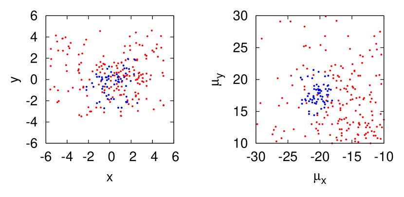
Figure 1: Positions (left) in pc relative to the center and proper motions (right) in mas/yr for the stars in the region of the open cluster IC 2391. Red circles indicate field stars and blue circles cluster members according to the method applied in this work.

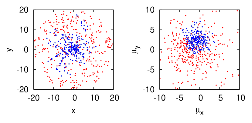
Figure 2: Same as Fig. 1, but for the open cluster NGC 2194.

we can see both positions and proper motions for the stars in the region of the open clusters IC 2391 and NGC 2194, respectively. We also show, in Figures 3 and 4,

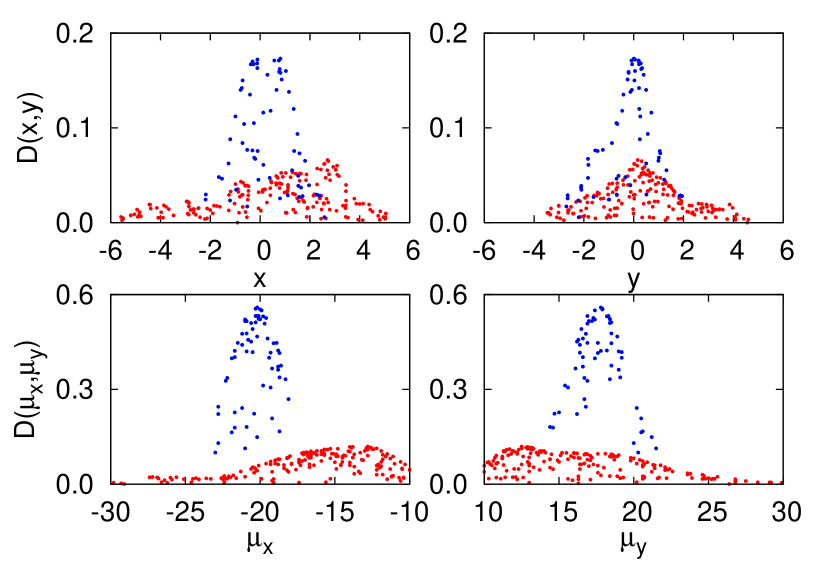
Figure 3: Probability density funcions for the stars in the region of the open cluster IC 2391. The two upper panels show the projections in $x$ and $y$ of the probability densities in the position space. The two lower panels are the projections in $\mu_{x}$ and $\mu_{y}$ of the probability densities in the proper motion space. Red circles refer to field stars and the blue ones to cluster members.

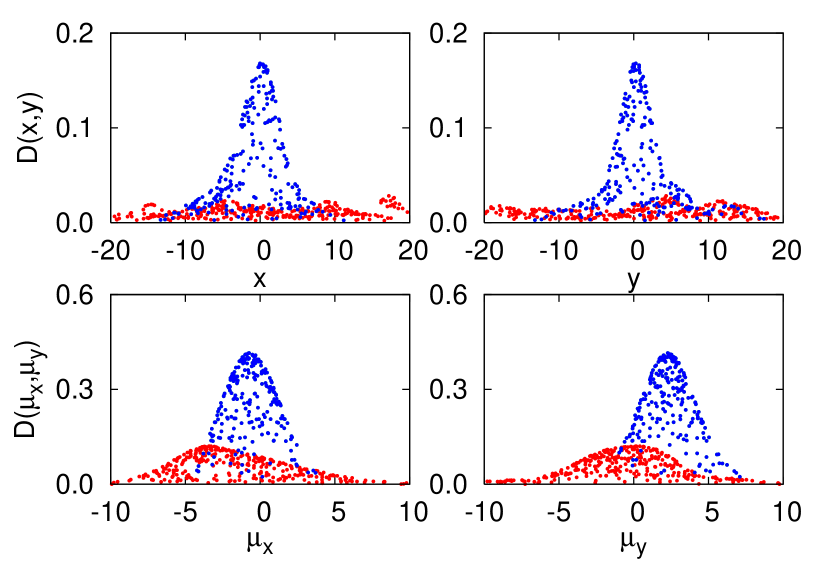
Figure 4: Same as Fig. 3, but for the open cluster NGC 2194.

the corresponding probability density funcions for the same two clusters. We see that both populations (field stars and cluster members) have been successfully separated by the algorithm. The spatial distribution of stars in IC 2391 is more irregular than in NGC 2194, but this is difficult to see from the spatial distribution because of the small number of members in IC 2391. However, the probability density functions allow a very easy visualization of the spatial structure. For example, two separate peaks are clearly visible in IC 2391 located at ($x$,$y$) positions close to (1,0) and (-0.5,0), and an additional weaker overdensity close to (0,-2). NGC 2194 exhibits a smoother distribution in the central region that becomes more irregular at the border of the cluster. For example, a small overdensity can be observed close to position (-5,5). Here we are showing the projected probability density funcions, obviously the three-dimensional display allows a better visualization of the cluster structure.

2.3 Comparison between the parametric and non-parametric methods

The methods for discriminating between cluster and field stars based on the proper motion distributions (Vasilevskis et al., 1958) use parametric Gaussian functions to represent the corresponding probability density functions (PDFs). Usually a circular Gaussian function is assumed for the PDF of the cluster whereas an elliptical one is adopted for the field. As mentioned in Section 2.2, this procedure may present problems if the underlying PDFs are far from being simple Gaussians, if the proper motion errors are anisotropic, or if the heterocedastic distance between the two stellar populations is small (see more detailed discussions in Cabrera-Caño & Alfaro, 1985, 1990; Platais, 2001; Balaguer-Núñez et al., 2004). In this case, a suitable option is to apply a non-parametric discriminating method that determines the PDFs empirically without a priori assumptions about the profile shapes. Additionally, even though the underlying PDFs may be well represented by Gaussians, if the cluster mean proper motion is very close to the maximum of the field distribution then the discriminating procedure becomes challengingly difficult. In fact, the discrimination becomes more difficult as the statistical distance between both populations decreases. To increase the statistical distance between cluster and field it becomes necessary to extend the dimension of the measurement space, and this is done by including the spatial coordinates in the non-parametric method used in this study (Cabrera-Caño & Alfaro, 1990).

In order to illustrate (and quantify) these arguments, let us compare the membership assignments obtained in this work (Section 2.2) with those obtained from the classical parametric method. We have used the algorithm proposed by Cabrera-Caño & Alfaro (1985) which estimates the parameters with a procedure more simple and efficient than that of Sanders (1971). Moreover, the algorithm first identifies outliers in the data in an objective way, i.e., in a distribution-free way not based on any previous parameters estimation. This is an important previous step because outliers make the distribution of field stars to be flatter than the actual one, modifying the final probabilities of cluster membership. In order to perform a better comparison we applied this parametric method to exactly the same data that we used for the non-parametric method. As representative examples, Figure 5

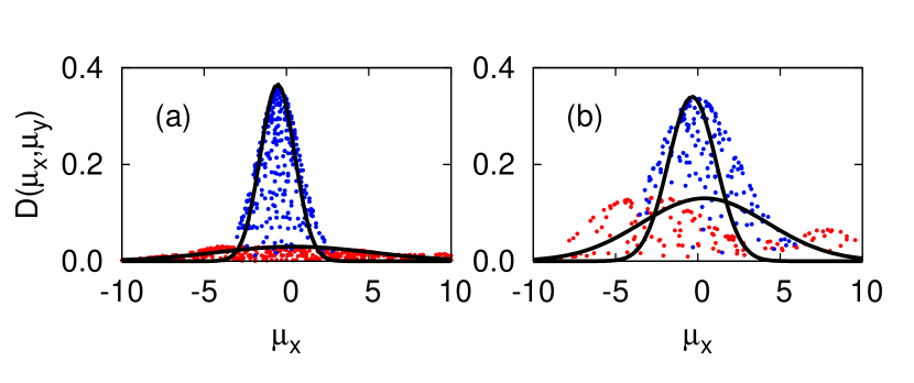
Figure 5: Probability density functions in the proper motion space (in mas/yr) for the stars in the region of (a) M 67 and (b) NGC 1513. Red and blue circles refer to field and cluster stars according to the non-parametric method, whereas thick black solid lines refer to the results of the parametric method.

shows the resulting PDFs in the proper motion space for two different open clusters (for a better clarity only the projection on the coordinate $\mu_{x}$ is shown). For the case of M 67 (Figure 5a) the parametric model finds the position of the cluster centroid at $\mu_{x,c}=-0.54$ and $\mu_{y,c}=+0.43$ with $\sigma_{c}=1.04$, and the field centroid at $\mu_{x,f}=+0.46$ and $\mu_{y,f}=+2.22$ with $\sigma_{x,f}=4.71$ and $\sigma_{y,f}=4.53$. Both parametric and non-parametric PDFs are similar to each other because cluster and field PDFs are different enough to allow an adequate separation of both populations. In fact, 93.67 % of the stars in the field of M 67 were assigned to the same population (cluster member or field star) by both methods. For NGC 1513 (Figure 5b) the parametric method finds the cluster centroid at $\mu_{x,c}=-0.34$ and $\mu_{y,c}=+0.53$ with $\sigma_{c}=1.45$, and the field at $\mu_{x,f}=+0.41$ and $\mu_{y,f}=+0.24$ with $\sigma_{x,f}=3.83$ and $\sigma_{y,f}=4.06$. For this case the statistical difference between both Gaussian PDFs is small in comparison with M 67 so that, in principle, it is more difficult to disentangle both populations. The differences between the parametric and non-parametric PDFs are more evident and only the 71.4 % were assigned to the same class by both methods. The difference in class assignments arises from the different PDFs in the proper motion space, but it equally arises from the fact that the non-parametric method also uses information from the position space: a star relatively far from the proper motion centroid might be classified as a probable cluster member if it was in a high density region in the corresponding spatial PDF.

The statistical separation between any two types of populations can be described through the Chernoff probabilistic distance (Chernoff, 1952), which is a measure of the difference between two probability distributions. We have calculated the Chernoff distance between the two Gaussian PDFs obtained by the parametric method. This was done for all the clusters in the sample to quantify the differences between the two stellar populations (cluster and field) in the porper motion space. Figure 6

Figure 6: Agreement in membership assignation between the parametric and non-parametric methods as a function of the Chernoff distance between cluster and field parametric probability density functions.

shows the percentage of stars that have obtained the same assignation (member or non-member) by both methods as a function of the Chernoff distance. The non-parametric method used in this work is robust in the sense that if cluster and field stars can be easily separated in the proper motion space then the results agree very well with those of the standar parametric method. For small Chernoff distances is more difficult to disentangle both stellar populations only from their proper motions. In this case, the non-parametric method has the advantage of using additional information from the star positions and then is able to provide a better discrimination.

3 Distribution of stars

We start by using the minimum spanning tree (MST) technique to analyse the distribution of stars in the clusters. The MST is the set of straight lines (called edges) connecting a given set of points without closed loops, such that the total edge length is minimum. Cartwright & Whitworth (2004) used this technique to study the distribution of stars in clusters introducing the dimensionless parameter $Q$. In order to calculate $Q$ we first need to determine the normalized correlation length $\overline{s}$, i.e. the mean separation between stars divided by the overall radius of the cluster. Next, from the MST we determine the normalized mean edge length $\overline{m}$, i.e. the mean length of the branches of the tree divided by $(A/N)^{1/2}$ where $A$ is the cluster area and $N$ the total number of stars. To estimate the area (and from that the radius) we use the strategy suggested by Schmeja & Klessen (2006), which consists in using the area of the convex hull, i.e. the minimum-area convex polygon containing the whole set of data points. Each one of these parameters ($\overline{s}$ and $\overline{m}$) cannot distinguish between a (relatively smooth) large-scale radial density gradient and a multiscale (fractal) subclustering. However, Cartwright & Whitworth (2004) showed that the combination $Q=\overline{m}/\overline{s}$ not only is able to distinguish between radial clustering and fractal type clustering but can also quantify them. We have generated two different sets of random three-dimensional distributions of points: one having a volume density of stars $n$ decreasing smoothly with the distance from the center $r$ as $n\propto r^{-\alpha}$ (Cartwright & Whitworth, 2004), and the other having fractal patterns according to a recipe that generates distributions with a well-defined fractal dimension $D_{f}$ (Sánchez & Alfaro, 2008). These random simulations were done 50 times, they were projected on random planes, and then we calculated the parameter $Q$ directly from the projected distributions. The overall results are shown in Figure 7.

Figure 7: Mean values of the parameter $Q$ as a function of the fractal dimension $D_{f}$ for projected fractals (open squares, bottom axis), and as a function of the index $\alpha$ for projected radial profiles (open circles, top axis). The bars are the corresponding standard deviations. The solid horizontal line indicates the value $Q=0.785$ for which both results converge to the homogeneous distribution case ($D_{f}=3$ and $\alpha=0$).

The value $Q=0.785$ (indicated as a horizontal line) separates radial clustering (open circles) from fractal clustering (open squares). Moreover, the value of $Q$ itself gives information about the value of $\alpha$ or $D_{f}$. We have to point out, however, that the uncertainties for the fractal distributions are rather large to determine in a precise way $D_{f}$ from the $Q$ value.

We applied this method to the sample of stellar clusters and the resulting $Q$ values are given in Table The spatial distribution of stars in open clusters. Stars in clusters with $Q>0.80$ are distributed following radial clustering profiles. For a better characterization of this kind of structure we have fitted King (1962) profiles to the radial density distributions of the cluster members (see Hillenbrand & Hartmann, 1998, for a discussion on the applicability of this kind of fit to open clusters). Before doing the fit we subtract from the cluster density function the maximum of the field density function, i.e. we perform the fit only for the stars in the cluster having probability densities above the maximum field density. Figure 8

Figure 8: Radial density profiles for the members of the open clusters IC 2391 (solid circles) and NGC 2194 (open circles). Dashed curves are the King profiles fitted up to the maximum density of the field stars.

shows the results for the same two example clusters shown in the previous figures (IC 2391 and NGC 2194). We performed this fit for all the clusters in our sample, even for the ones that do not follow smooth profiles. From the best fits we obtained the core ($R_{c}$) and tidal ($R_{t}$) radii. Both radii are shown in Table The spatial distribution of stars in open clusters. Clearly, this fit is unrealistic when the cluster exhibits a high degree of substructure but, even in this case, it allows us to estimate the cluster radius ($R_{t}$) in a homogeneous way for the 16 clusters in the sample.

Eight of the clusters of our sample (IC 2391, M 34, NGC 581, NGC 1513, NGC 1647, NGC 1817, NGC 4103, and NGC 6530) have structure parameter values close to, or below, the threshold value $Q\simeq 0.80$. These clusters would follow fractal-like patterns but, as mentioned before, to infer the fractal dimension from the $Q$ value is quite uncertain. For these clusters, we choose to estimate the degree of clumpiness by calculating the correlation dimension ($D_{c}$). For this we use an algorithm that estimates $D_{c}$ in a reliable (precise and accurate) way (Sánchez et al., 2007a; Sánchez & Alfaro, 2008). The algorithm avoids the usual problems that arise at relatively large scales (boundary effects) and small scales (finite-data effects) by using objective and suitable criteria. Moreover, an uncertainty associated to each $D_{c}$ value is estimated using bootstrap techniques. The application of this algorithm to the eight clusters having fractal structure yields the results shown in Table 2.

4 Discussion

Now we proceed to examine the dependence of $Q$ on the cluster age in order to compare it with the trend mentioned by other authors. This kind of dependence has been suggested not only for stellar clusters (Schmeja & Klessen, 2006; Schmeja et al., 2008) but also for the distribution of young stars in the Gould Belt (Sánchez et al., 2007a), the distribution of young clusters in the solar neighborhood (de La Fuente Marcos & de La Fuente Marcos, 2006), and the distribution of stars (Bastian et al., 2009; Gieles et al., 2008; Odekon, 2008) and HII regions (Sánchez & Alfaro, 2008) in external galaxies. A slight positive trend is apparent when we plot $Q$ versus $\log(T)$, i.e. fractal clusters tend to be younger than clusters having radial density profiles. However, the statistical analysis indicates that there is no significant correlation between this structure parameter and cluster age, neither for the full sample nor for the fractal clusters and density profile clusters considered individually. From simple arguments one would expect that $Q$ increases with time for each cluster. Gravitationally unbound cluster will tend to nearly homogeneous distributions ($Q=0.79$, $D_{c}=2.0$) because of the dispersal of stars, whereas self-gravity will lead to more centrally peaked distributions in bound clusters. It could take several crossing times to reach an equilibrium state and/or to eliminate the original distribution (Bonnell & Davies, 1998; Goodwin & Whitworth, 2004), although maybe it could take only a crossing time (Bastian et al., 2009). The typical crossing time in open clusters is of the order of $10^{6}$ years (Lada & Lada, 2003) but, assuming nearly the same typical velocity dispersion, the crossing time is roughly proportional to the cluster size. Let us consider the new variable, $T/R_{t}$ (in yr/pc), which is proportional to time measured in crossing time units. In this case we do observe the correlation

$$Q=(0.07\pm 0.03)\log(T/R_{t})+(0.35\pm 0.21)\ \ \ ,$$

which is significant at 96% confidence level. This result is shown in Figure 9.

Figure 9: Structure parameter $Q$ as a function of the logarithm of age divided by the tidal radius, which is nearly proportional to age in crossing time units. The dashed line at $Q=0.8$ roughly separates radial from fractal clustering, and the solid line is the best linear fit.

Previous detailed studies on the fractal properties of projected distributions of points (Sánchez et al., 2007a; Sánchez & Alfaro, 2008) have shown that the uncertainty associated with $D_{c}$ depends on the number of available data. Moreover, when the number of data points is too low ($N\lesssim 200$) a bias in the mean $D_{c}$ values is produced. We performed a similar analysis for the parameter $Q$ using the simulated fractals. We verified that the mean measured value of $Q$ tends to be overestimated if $N\lesssim 200$, and the bias was higher as the fractal dimension (and therefore $Q$) decreased. For the extreme case studied here ($D_{f}=2$), the maximum difference between the mean value of $Q$ for well-sampled point sets (namely $Q=0.576$, see Figure 7) and fractals having $N\sim 200$ data points was $\Delta Q\simeq 0.06$. The important point here is that if this kind of bias is present in our results, then the correlation shown in Figure 9 might be reinforced.

The structure parameter is shown in Figure 10

Figure 10: Structure parameter as a function of the concentracion parameter of the King model. The dashed line ($Q=0.8$) roughly separates clusters with well-defined radial density profiles (open circles) and clusters with substructures (filled circles). The solid line is the best linear fit for the upper subsample.

as a function of the concentration parameter of the King model. Interestingly, the behaviors of the subsamples $Q>0.8$ and $Q\leq 0.8$ are clearly differentiated. $Q$ correlates strongly with the concentration for cluster with well-defined radial density profiles, the best linear fit (solid line in Fig. 10) being

$$Q=-(0.66\pm 0.20)\log(R_{t}/R_{c})+(1.24\pm 0.10)\ \ \ ,$$

with a confidence level greater than 98%. Otherwise, the fractal-like subsample does not show any correlation at all.

As we have seen, there seems to be some evidence that young clusters tend to distribute their stars following fractal patterns whereas older clusters tend to exhibit centrally concentrated structures. But this is only an overall trend. Note, for example, that NGC 1513 and NGC 1647 have both $Q\sim 0.7$ with ages of $T\gtrsim 100$ Myr. The advantage of analyzing the clustering properties via the correlation dimension is that, apart from directly measuring the fractal dimension, the assignment of an associated uncertainty allows us to know the reliability of each measurement. The results of $D_{c}$ for the clusters having $Q\lesssim 0.8$ are shown in Table 2. The best linear fit between the fractal dimension and the age is:

$$D_{c}=(0.14\pm 0.05)\log(T)+(0.77\pm 0.39)\ \ \ ,$$

significant at a confidence level of 97%. If we use $T/R_{t}$ instead $T$ the fit becomes:

$$D_{c}=(0.11\pm 0.04)\log(T/R_{t})+(1.08\pm 0.30)\ \ \ ,$$

significant at a level of 96%. This last fit is shown in Figure 11,

Figure 11: Calculated correlation dimension as a function of the logarithm of age divided by the tidal radius. The solid line is the best linear fit.

where we can see that the correlation looks very good by eye. The point farthest from the best-fit line is the cluster IC 2391, which has the smallest number of members ($N_{s}=62$) and the largest uncertainty in $D_{c}$ ($0.2$). If the result for this cluster is biased, then the fractal dimension should be higher than the value reported here and the correlation should be even stronger. An important aspect to be mentioned is that there exist stellar clusters as old as $\sim 100$ Myr that have not totally destroyed their clumpy substructure. This is a particularly meaningful result that gives some observational support to recent simulations of the dynamical evolution of young clusters (Goodwin & Whitworth, 2004).

We have already mentioned that converting from two-dimensional to three-dimensional fractal dimensions increases the associated uncertainties. However, it is interesting to note that according to our previous works (Sánchez et al., 2007a; Sánchez & Alfaro, 2008), clusters with the smallest correlation dimensions ($D_{c}=1.74$) would have three-dimensional fractal dimensions around $D_{f}\sim 2.0$. This values is considerably smaller than the average value $D_{f}\simeq 2.6-2.7$ estimated for the interstellar medium in recent studies (Sánchez et al., 2005, 2007b). Perhaps the development of some kind of substructure in initially more homogeneous clusters observed in some simulations could explain this difference, although some coherence in the initial velocity dispersion would be necessary (Goodwin & Whitworth, 2004). Another plausible explanation is that this difference is a consequence of a more clustered distribution of the densest gas at the smallest spatial scales in the molecular cloud complexes, according to a multifractal scenario for the interstellar medium (Chappell & Scalo, 2001; Tassis, 2007). The problem is complex because it depends on: (a) the initial distribution of gas and dust in the parent cloud, (b) the way and degree in which this information is transferred to the new-born stars, and (c) how, and how fast, this initial star distribution evolves. Each one of these factors will depend to a greater or lesser extent on the involved physics and environmental variables. These points clearly require more investigation.

5 Conclusions

We have characterized quantitatively the distribution of stars in a relatively large sample of open clusters (a total of 16) spanning a wide range of ages. Membership probabilities were obtained by applying a non-parametric method that does not make any assumption on the underlying star distribution. This is a crucial point to avoid possible bias introduced by the cluster member selection process. We found evidence that stars in young clusters tend to be distributed following clustered, fractal-like patterns, whereas older clusters tend to exhibit radial star density profiles. This result supports the idea that stars in new-born cluster likely follow the fractal patterns of their parent molecular clouds, and that eventually evolve toward more centrally concentrated structures (see also Schmeja & Klessen, 2006). However, we have also obtained some other interesting results: (a) there exists a strong correlation between the structure parameter $Q$ and the concentration parameter of the King model $\log(R_{t}/R_{c})$ for the clusters with well-defined radial density profiles, (b) clusters as old as $\sim 100$ Myr can exhibit a high degree of spatial substructure, and (c) there is a significant correlation between fractal dimension and age for the cluster with fractal distribution of stars. Additionally, we find that the smallest values of the corresponding three-dimensional fractal dimensions are $D_{f}\sim 2.0$, which is considerably smaller than the value $D_{f}\simeq 2.6-2.7$ estimated for the average interstellar gas distribution. If this is a general result, then some further explanation would be required.

Table 1: Properties of the clusters in the sample

Name	$\log(T)$	$D$	$N_{d}$	$N_{s}$	$Q$	$R_{c}$	$R_{t}$	Ref.
IC 2391	7.661	175	6847	62	0.77	1.46	2.65	(1)
M 67	9.409	908	1046	354	0.98	2.21	5.92	(2)
M 11	8.302	1877	872	289	1.02	1.98	4.49	(3)
M 34	8.249	499	630	181	0.80	0.11	1.73	(4)
NGC 188	9.632	2047	7771	1459	0.91	2.90	10.57	(5)
NGC 581	7.336	2194	2387	526	0.76	1.38	11.86	(6)
NGC 1513	8.110	1320	332	156	0.72	1.55	7.73	(7)
NGC 1647	8.158	540	2220	683	0.70	1.23	8.86	(8)
NGC 1817	8.612	1972	810	277	0.79	3.39	11.97	(9)
NGC 1960	7.468	1318	1190	311	0.87	2.96	8.77	(10)
NGC 2194	8.515	3781	2233	228	0.85	3.17	10.31	(10)
NGC 2548	8.557	769	501	168	0.90	2.61	9.16	(11)
NGC 4103	7.393	1632	4379	799	0.78	0.72	10.74	(12)
NGC 4755	7.216	1976	384	196	0.94	1.11	3.50	(12)
NGC 5281	7.146	1108	314	80	0.84	0.62	2.44	(12)
NGC 6530	6.867	1330	364	145	0.67	1.43	7.47	(13)

References. — (1) Platais et al. (2007); (2) Zhao et al. (1993); (3) Su et al. (1998); (4) Jones & Prosser (1996); (5) Platais et al. (2003); (6) Sanner et al. (1999); (7) Frolov et al. (2002); (8) Geffert et al. (1996); (9) Balaguer-Núñez et al. (2004); (10) Sanner et al. (2000); (11) Wu et al. (2002); (12) Sanner et al. (2001); (13) Zhao et al. (2006).

Table 2: Calculated Correlation Dimensions

Name	$D_{c}$
IC 2391	$1.74\pm 0.20$
M 34	$2.04\pm 0.05$
NGC 581	$1.79\pm 0.06$
NGC 1513	$1.82\pm 0.09$
NGC 1647	$1.94\pm 0.02$
NGC 1817	$1.94\pm 0.04$
NGC 4103	$1.85\pm 0.04$
NGC 6530	$1.74\pm 0.09$

References

- Balaguer-Núñez et al. (2004) Balaguer-Núñez, L., Jordi, C., Galadí-Enríquez, D., & Zhao, J. L. 2004, A&A, 426, 819
- Ballesteros-Paredes et al. (2006) Ballesteros-Paredes, J., Gazol, A., Kim, J., Klessen, R. S., Jappsen, A.-K., & Tejero, E. 2006, ApJ, 637, 384
- Ballesteros-Paredes et al. (2007) Ballesteros-Paredes, J., Klessen, R. S., Mac Low, M.-M., & Vazquez-Semadeni, E. 2007, Protostars and Planets V, 63
- Bastian et al. (2009) Bastian, N., Gieles, M., Ercolano, B., & Gutermuth, R. 2009, MNRAS, 392, 868
- Bastian et al. (2008) Bastian, N., Gieles, M., Goodwin, S. P., Trancho, G., Smith, L. J., Konstantopoulos, I., & Efremov, Y. 2008, MNRAS, 389, 223
- Bate et al. (1998) Bate, M. R., Clarke, C. J., & McCaughrean, M. J. 1998, MNRAS, 297, 1163
- Bonnell & Davies (1998) Bonnell, I. A., & Davies, M. B. 1998, MNRAS, 295, 691
- Bonnell et al. (2003) Bonnell, I. A., Bate, M. R., & Vine, S. G. 2003, MNRAS, 343, 413
- Cabrera-Caño & Alfaro (1985) Cabrera-Caño, J., & Alfaro, E. J. 1985, A&A, 150, 298
- Cabrera-Caño & Alfaro (1990) Cabrera-Caño, J., & Alfaro, E. J. 1990, A&A, 235, 94