Dilute gas of ultracold two-level atoms inside a cavity: generalized Dicke model

Abstract

We consider a gas of ultracold two-level atoms confined in a cavity, taking into account for atomic center-of-mass motion and cavity mode variations. We use the generalized Dicke model, and analyze separately the cases of a Gaussian, and a standing wave mode shape. Owing to the interplay between external motional energies of the atoms and internal atomic and field energies, the phase-diagrams exhibit novel features not encountered in the standard Dicke model, such as the existence of first and second order phase transitions between normal and superradiant phases. Due to the quantum description of atomic motion, internal and external atomic degrees of freedom are highly correlated leading to modified normal and superradiant phases.

I Introduction

Progress in trapping and cooling of atomic gases meystre made it possible to coherently couple a Bose-Einstein condensate to a single cavity mode bec_cav . These experiments pave the way to a new sub-field of AMO physics; many-body cavity quantum electrodynamics. In the ultracold regime, light induced mechanical effects on the matter waves lead to intrinsic non-linearity between the matter and the cavity field ritsch0 ; jonas1 . In particular, the non-linearity renders novel quantum phase transitions (QPT) qpt , see cavity . Such non-linearity, due to the quantized motion of the atoms, is absent in the, so called, standard Dicke model (DM). Explicitly, the DM describes a gas of $N$ non-moving two-level atoms interacting with a single quantized cavity mode dicke . The interplay between the field intensity/energy, the free atom energy, and the interaction energy leads to a quantum phase transition (DQPT) in the DM. Motivated by the novel phenomena arising from a quantized treatment of atomic motion, it is highly interesting to extend the DM to include atomic motion on a quantum scale, and in particular to analyze how it affects the nature of the DQPT. It is clear that such generalization of the DM results in new aspects of the system properties. The atomic motion is directly affected by the shape of the field induced potentials, which in return is determined by the system parameters and the field intensity. In addition to the terms contributing to the total energy in the regular DM, in this model we have to take into account for the motional energy of the atoms. This enters in a non-trivial way since the interaction energy depends on the motional states of the atoms.

The DM was first introduced in quantum optics to describe the full collective dynamics of atoms in a high quality cavity. The DM Hamiltonian, given in the rotating wave approximation (RWA), reads

$$H_{D}=\hbar\omega\hat{a}^{\dagger}\hat{a}+\frac{\hbar\Omega}{2}\sum_{i=1}^{N}\hat{\sigma}_{i}^{z}+\frac{\hbar\lambda}{\sqrt{N}}\sum_{i=1}^{N}\left(\hat{a}^{\dagger}\hat{\sigma}_{i}^{-}+\hat{\sigma}_{i}^{+}\hat{a}\right).$$ (1)

Here, the boson ladder operators $\hat{a}^{\dagger}$ and $\hat{a}$ create and annihilate a photon of the cavity mode, the Pauli $\hat{\sigma}_{i}$-operators act on atom $i$, $\omega$, $\Omega$ and $\lambda$ are the mode and atomic transition frequencies and effective atom-field coupling respectively. The DM is a well defined mathematical model for any value of its parameters. Note, however, that whether this model describes faithfully some physical situation for any choice of parameters is not guaranteed. For moderate $\lambda$, the DM appropriately describes the dynamics of atoms coupled to the cavity field, and it has been thoroughly discussed in terms of collapse-revivals cr , squeezing squeez , entanglement ent and state preparation stateprep . Considerable interest, however, has been devoted to the normal-superradiant phase transition hepp ; density ; orszag .

In the thermodynamic limit ($N,V\rightarrow\infty$, $N/V=\mathrm{const.}$) the system exhibits a non-zero temperature phase transition between the normal phase and the superradiant phase. In the normal phase, all atoms are in their ground state and the field in vacuum, while the superradiant phase is characterized by a non-zero field and a macroscopic excitation of the matter. Its critical coupling and critical temperature are hepp

$$\begin{array}[]{l}\displaystyle{\lambda_{c}=\sqrt{\Omega\omega}},\\ \\ \displaystyle{(k_{B}T_{c})^{-1}=\frac{2\omega}{\Omega}\mathrm{arctanh}\left(\frac{\Omega\omega}{\lambda^{2}}\right)}.\end{array}$$ (2)

As was shown in density , the critical coupling can be seen as a condition on the atomic density $\rho=N/V$. Interestingly, the DQPT is of second order nature without the RWA, while it is first order if the RWA has been imposed 1st . The corrections due to the RWA to various physical observables have been considered hioe ; orszag .

More detailed analysis about miscellaneous aspects of the DQPT have been presented in numerous publications. Especially various extensions ext ; onePT as well as approximate methods approx concerning the DQPT has been outlined. Recently, C. Emary and T. Brandes applied the algebraic Holstein-Primakoff boson representation on the DM. The method turned out to be very powerful and have since then been applied frequently to the DM alg .

Despite the numerous publications on the DQPT, the existence of this phase transition was widely discussed. If the two-level atoms in the DM correspond to atoms in a ground and excited state, and the transition is direct, then quantum mechanics forbids the transition. This can be seen either by realizing the necessity of adding the, so called, $A^{2}$-term to the Hamiltonian, or by employing sum rules to bound the coefficients in the Dicke model to the ”trivial” thermodynamical phase a2 . The argumentation of Ref. a2 can be generalized to a quite general no-go theorem for the DQPT nogo , but it does not apply if the two level atoms in the DM correspond to atoms in two excited states, such as Rydberg states, or if the transition is not direct.

One valuable step towards an experimental realization of the DQPT was taken in relation with Ref. carmichael , where typical experimental parameters as well as losses were included. These authors considered the two levels coupled by a non-resonant Raman transition. In such conditions the atom-field coupling $\lambda$ can be tuned more or less independently of the $A^{2}$ term in an effective two-level model, and one can reach the regime of DQPT. This paper, however, considers a situation in which atomic motion can be neglected due to high temperatures, e.g. the standard DQPT. Alternative situation, in which the atomic motion could be neglected, would be to consider quantum dots interacting with a cavity mode onePT ; JJ .

In this paper we extend the DM to take into account for atomic motion in a fully quantum mechanical description. The atomic motion then introduces an additional degree of freedom to the problem, leading to novel appearances of the system phase diagrams. The gas is assumed dilute such that atom-atom scattering can be neglected, and that the motion is restricted to one dimension due to tight confinement in the remaining two directions via external trapping. Furthermore, the atoms are assumed trapped by the cavity field itself. Consequently, a normal-superradiant QPT is not possible, since for a vanishing field the atomic trapping capability is lost. However, we may assume a lowest bound of the field such that at least one bound state of the trapping ”potential” is guaranteed. This can be achieved by an external pumping of the cavity, which imposes a non-vanishing cavity field. Our research is partly carried out in the adiabatic regime, motivated by the ultracold atoms considered and its justification is numerically verified. In this adiabatic regime, the problem relaxes to solving a 1-D time-independent Schrödinger equation. In particular we study the case of a Gaussian mode profile utilizing this adiabatic method. The situation with a standing wave mode profile is also considered, however using a full numerical rather than adiabatic approach. For a Gaussian profile the number of bound states is crucial for the thermodynamics, and we find great divergences from the regular DM. Among these are the existence of both first and second order QPT’s and multiple superradiant phases. The second, standing wave mode, shows slight similarities to the model of onePT but the QPT is found to be of second order, and the PT survives for zero temperature and finite $\omega$ opposite to the regular DQPT.

The paper is organized as follows. In the next section we present the generalized DM which includes the motion of the atom. The adiabatic diagonalization of the single particle Hamiltonians utilized for the Gaussian mode profile is introduced and the general expression for the partition function given. The following Sec. III considers the situation of a Gaussian mode profile. We thoroughly discuss the importance of bound states. Section IV instead considers a standing wave mode profile in a fully numerical fashion. In the appendix, however, we derive analytical expressions in the regimes of tight binding which enables us with various asymptotic properties. Last we conclude with a summery in Sec. V.

II Generalized Dicke model and its partition function

We consider an gas of $N$ ultracold identical two-level atoms, with mass $m$ and energy level separation $\hbar\Omega$, interacting with a single cavity mode with frequency $\omega$. For a low temperature gas we include atomic center-of-mass motion and mode variation. In the dipole and rotating wave approximation, the extended DM becomes

$$H\!=\!\omega\hat{a}^{\dagger}\hat{a}+\!\sum_{i=1}^{N}\!\left[\frac{\hat{p}_{i}^{2}}{2}+\!\frac{\Omega}{2}\hat{\sigma}_{i}^{z}+\frac{g(\hat{x}_{i})}{\sqrt{V}}\!\left(\hat{a}^{\dagger}\hat{\sigma}_{i}^{-}+\hat{\sigma}_{i}^{+}\hat{a}\right)\!\right]\!.$$ (3)

Here, $\hat{p}_{i}$ and $\hat{x}_{i}$ the scaled center-of-mass momentum and position of atom $i$ respectively, $g(\hat{x})$ the effective position-dependent atom-field coupling and $V$ is the mode volume. Throughout the paper we will use scaled variables such that $\hbar=m=1$. The case of a single atom is given by the generalized Jaynes-Cummings Hamiltonian studied by numerous authors potential ; effmass .

In the thermodynamic limit we let $V\rightarrow\infty$ and $N\rightarrow\infty$ such that the atomic density is fixed; $\rho=N/V\equiv\rho_{0}$. The partition function reads

$$Z=\mathrm{Tr}\Big{[}\mathrm{e}^{-\beta H}\Big{]},$$ (4)

where $\beta^{-1}=T$ and $T$ is the scaled temperature and the trace is over the field and atomic degrees of freedom. It is convenient to perform the trace of the field in terms of Glauber’s coherent states, $\hat{a}|\alpha\rangle=\alpha|\alpha\rangle$. In the thermodynamic limit one may replace $\hat{a}\rightarrow\alpha$ and $\hat{a}^{\dagger}\rightarrow\alpha^{*}$ in the evaluation of the partition function hepp . In other words; in the large atom number limit the photon ladder operators, or more precisely $\hat{a}/\sqrt{N}$ and $\hat{a}^{\dagger}/\sqrt{N}$, can be treated as commuting operators. Using the fact that atomic operators mutually commute between themselves, for example $[\hat{x}_{i},\hat{p}_{j}]=i\delta_{ij}$, the partition function can be written

$$Z=\int\frac{d^{2}\alpha}{\pi}\,\mathrm{e}^{-\beta\omega|\alpha|^{2}}\left\{\mathrm{Tr}\Big{[}\mathrm{e}^{-\beta h(\alpha)}\Big{]}\right\}^{N},$$ (5)

where the integration is over the whole complex $\alpha$-plane and

$$h(\alpha)=\frac{\hat{p}^{2}}{2}+\frac{\Omega}{2}\hat{\sigma}^{z}+\frac{g(\hat{x})\sqrt{\rho_{0}}}{\sqrt{N}}\left(\alpha\hat{\sigma}^{+}+\alpha^{*}\hat{\sigma}^{-}\right).$$ (6)

In the sense of ultracold atoms as considered here, the kinetic energy of the atoms is assumed smaller than the effective potential energy. Provided that the adiabatic potentials do not cross, it is then legitimized to perform an adiabatic diagonalization of the internal states ad . In this regime, the single particle Hamiltonian relaxes to two decoupled adiabatic ones

$$\begin{array}[]{lll}h_{ad}^{\pm}(|\alpha|)&=&\displaystyle{\frac{\hat{p}^{2}}{2}+V_{ad}^{\pm}(\hat{x},|\alpha|^{2})}\\ \\ &\equiv&\displaystyle{\frac{\hat{p}^{2}}{2}\pm\sqrt{\frac{\Omega^{2}}{4}+\frac{g^{2}(\hat{x})\rho_{0}}{N}|\alpha|^{2}}}.\end{array}$$ (7)

This approximation will be imposed in the next section considering a Gaussian mode profile. However, in the proceeding section dealing with the standing wave mode such an approach is not advocate, since then the curve crossings between the adiabatic potentials break adiabaticity ad . The justification of the adiabatic approximation applied to the Gaussian mode profile will be discussed in the end of next Section. Within this regime, the problem has become one of solving for the eigenvalues of two time-independent decoupled Schrödinger equations. The adiabatic Hamiltonians depend solely on the norm $|\alpha|$ and in polar coordinates the angle part can therefore be integrate out. By denoting the eigenvalues $E_{n}^{\pm}(r)$ respectively, where $r=|\alpha|$ and $n$ is a quantum number/numbers that can be either discrete and/or continuous, we get the adiabatic partition function

$$Z_{ad}\!=\!2\!\int_{0}^{\infty}\!dr\,r\mathrm{e}^{-\beta\omega r^{2}}\!\left\{\mathrm{Tr}\Big{[}\mathrm{e}^{-\beta E_{n}^{+}(r)}\Big{]}\!+\!\mathrm{Tr}\Big{[}\mathrm{e}^{-\beta E_{n}^{-}(r)}\Big{]}\!\right\}^{N}.$$ (8)

Without loss of generality we can choose $\rho_{0}=1$ as it only scales the effective atom-field coupling. It is worth mentioning that the numerics deal with exponentially large numbers, especially for small temperatures, which restrict the analysis to certain ranges.

III Transversal thermodynamics

III.1 Derivation of the partition function for transversal motion

A Fabry-Perot cavity has eigenmodes that are, to a good approximation, Gaussian in the transverse and harmonic in the longitudinal direction. Assuming an external deep trap in the longitudinal direction and one transverse direction, we may consider the one dimensional problem in which the atom field coupling has a spatial Gaussian shape. As is well known potential , and seen from Eq. (7), only atoms in the ”adiabatic” internal state corresponding to the Hamiltonian $h_{ad}^{-}(r)$ will feel an attractive potential, while the others will be scattered away from the cavity field. We therefore consider only a sub ”quasi” Hilbert space containing the bound states $E_{n}^{-}(r)$ of

$$h_{ad}^{-}(r)=\frac{\hat{p}^{2}}{2}-\sqrt{\frac{\Omega^{2}}{4}+\frac{\lambda^{2}r^{2}}{N}\exp\left(-2\frac{x^{2}}{\Delta_{x}^{2}}\right)},$$ (9)

where $\Delta_{x}$ is the transverse mode width.

In order to proceed in an analytic way, we make the following approximate ansatz,

$$\sqrt{\frac{\Omega^{2}}{4}+\frac{\lambda r^{2}}{N}\exp\left(-2\frac{x^{2}}{\Delta_{x}^{2}}\right)}\approx\epsilon_{0}+U_{0}\mathrm{sech}^{2}(qx).$$ (10)

The unknown constants are determined from the conditions: (i) The two functions have the same asymptotic values for $x\rightarrow\pm\infty$, (ii) their maximum are the same and (iii) they share the same FWHM. Explicitly this yields

$$\begin{array}[]{l}\displaystyle{\epsilon_{0}=\frac{\Omega}{2}},\\ \\ \displaystyle{U_{0}(r^{2})=\sqrt{\frac{\Omega^{2}}{4}+\frac{\lambda^{2}r^{2}}{N}}-\frac{\Omega}{2}},\\ \\ \displaystyle{q_{r^{2}}=\frac{\sqrt{2}\,\mathrm{arcsech}\left(\sqrt{1/2}\right)}{\Delta_{x}\sqrt{\ln\left[\frac{4\lambda^{2}r^{2}}{N\left(\left(\sqrt{\frac{\Omega^{2}}{4}+\frac{\lambda^{2}r^{2}}{N}}+\frac{\Omega}{2}\right)^{2}-\Omega^{2}\right)}\right]}}}.\end{array}$$ (11)

The bound eigenvalues of the Hamiltonian

$$h_{ad}^{-}(r)=\frac{\hat{p}^{2}}{2}-\frac{\Omega}{2}-U_{0}(r^{2})\,\mathrm{sech}^{2}(q_{r^{2}}x)$$ (12)

are known to be ll

$$E_{n}^{-}(r^{2})=-\frac{\Omega}{2}-\frac{q_{r^{2}}^{2}}{8}\left[-(1+2n)+\sqrt{1+\frac{8U_{0}(r^{2})}{q_{r^{2}}^{2}}}\right]^{2}.$$ (13)

Let us introduce the number of bound states, for a given set of parameters, as $\tilde{N}$ and define the function

$$g_{1}(r^{2})=\sum_{n=0}^{\tilde{N}}\mathrm{e}^{-\beta E_{n}^{-}(r^{2})}.$$ (14)

With this, the partition function (8), considering only bound states, becomes

$$Z_{ad}=2\int_{0}^{\infty}dr\,r\mathrm{e}^{-\beta\omega r^{2}+N\ln\big{[}g_{1}(r^{2})\big{]}}.$$ (15)

By the variable substitution $y=r^{2}/N$ we get

$$Z_{ad}=N\int_{0}^{\infty}dy\,\mathrm{e}^{N\big{[}-\beta\omega y+\ln\left[g_{1}(y)\right]\big{]}}.$$ (16)

In the thermodynamic limit, this integral is solved by the saddle point method saddle

$$Z_{ad}=N\frac{C_{1}}{\sqrt{N}}\max_{0\leq y\leq\infty}\left\{\mathrm{e}^{N\big{[}-\beta\omega y+\ln\left[g_{1}(y)\right]\big{]}}\right\},$$ (17)

where $C_{1}$ is a constant. Note that $y$ has the meaning of scaled field intensity.

One obstacle of the above model already mentioned in the introduction, is the fact that for a shallow potential well the number of bound states will vanish. In this limit, the cavity field can no longer serve as a trap for the atoms. Consequently the ground state is the one of zero atoms, and we cannot have a proper thermodynamic limit $N\rightarrow\infty$. We therefore add the constrain of a minimum of one bound state is assumed. This can be met experimentally by including an external driving of the cavity mode, so that the field is non-zero throughout. Thus, the ”normal” phase will contain a non-zero cavity field which is sustained by the external pumping. We have numerically checked that this does not introduce any significant changes of the analysis.

For the number $\tilde{N}$ of bound states, we have

$$(1+2\tilde{N})<\sqrt{1+\frac{8U_{0}(y)}{q_{y}^{2}}}.$$ (18)

Naturally, $\tilde{N}$ depends on the system parameters. As $\tilde{N}$ is an integer, a change in the system parameters may bring about jumps between integer numbers of $\tilde{N}$. This will cause discontinuities in the function $g_{1}$. Letting $\tilde{N}=1$ we find $U_{0}(y)>q_{y}^{2}$. For small fields, $y\rightarrow 0$, the potential amplitude $U_{0}$ vanishes and the bound states cease to exist. However, for small but non-zero fields, the above inequality may be met for large couplings $\lambda$ and widths $\Delta_{x}$.

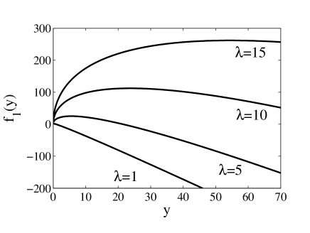
Figure 1: Examples of the free energy per particle $f_{1}(y)$ of Eq. (19). The inserted numbers give the couplings $\lambda$ and the other dimensionless parameters are $\Omega=\omega=1$, $\Delta_{x}=2$ and $T=0.2$.

III.2 Numerical results

To study Eq. (17), we analyze the parameter dependence of the function

$$f_{1}(y)=-\beta\hbar\omega y+\ln\left[g_{1}(y)\right].$$ (19)

Note that $f_{1}(y)$ is the free energy per particle, given a scaled field intensity $y$. Let us briefly discuss characteristics of $f_{1}(y)$ before approaching it numerically. The first part arises from the bare field, and it is energetically favorable to have a vanishing field. The second part contains the atom-field interactions plus kinetic and potential atomic energies. The interaction energy enters indirectly into the atomic potential part. Increasing the field amplitude deepens the potential well and therefore lowers the energy, and it is therefore more beneficial to have a large field. The two terms therefore compete, and in particular, the location of the maximum of $f_{1}(y)$ depends on the particular system parameters used. Thus, atomic motion, directly related to the shape and depth of the adiabatic potential, is a crucial ingredient for the QPT. If the smallest possible $y$ maximizes the function, the system is said to be in a ”normal” phase (in quotes because the field is still non-zero to guarantee at least one bound state), while if a non-minimal $y$ is optimal the system is in a superradiant phase. In the limit of large $y$, the second term diverges as $\ln\left[g_{1}(y)\right]\sim\sqrt{y}$ while the first term goes as $\sim-y$, and we conclude that a maximum of $f_{1}(y)$ is only obtained for a finite $y$. These reflections are numerically verified in Fig. 1 showing $f_{1}(y)$ for four different couplings $\lambda$. We see that there is a critical coupling $\lambda_{c}$ for which $\lambda<\lambda_{c}$ the system is in a ”normal” phase and for $\lambda>\lambda_{c}$ it is in a superradiant phase.

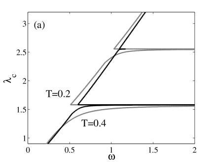
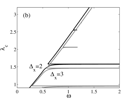
Figure 2: The critical atom-field coupling $\lambda_{c}$ for the potential well (10) as function of $\omega$. In (a) gray curve corresponds to $T=0.2$ and black curve to $T=0.4$, while in (b) for gray curve $\Delta_{x}=3$ and for black curve $\Delta_{x}=2$. In both plots $\Omega=1$, and in (a) $\Delta_{x}=2$ and in (b) $T=0.2$. All parameters are dimensionless.

In Fig. 2 we display the critical coupling $\lambda_{c}$ as function of $\omega$ while keeping the other parameters fixed. In (a) we present two examples for different $T$ and in (b) two examples for different $\Delta_{x}$. For the plots, the minimum $y$ is taken so that there is at least one bound state in the well. To the left of the curves the phase is superradiant, while to the right it is ”normal”. The structure of the phase diagram is clearly different from the one of the regular DM in which, at zero temperature, $\lambda_{c}\sim\sqrt{\omega}$. For certain couplings $\lambda_{s}$, the system is always in a superradiant phase independent of $\omega$. The location of these resonances are insensitive to the temperature but not to trap width $\Delta_{x}$. The “sharpness” of these points makes it possible to have a ”normal”-superadiant-”normal” QPT by fixing all parameters but the coupling $\lambda$ which is varied around $\lambda_{s}$. This novel feature comes about due to the varying number of bound states $\tilde{N}$ in the well. For say $\omega\approx 1$ and a weak coupling, the system is in the ”normal” phase with only one bound state. As $\lambda$ is increased the system goes through a QPT into a superradiant phase. A closer numerical study shows that this QPT is caused by the sudden change of going from one to two bound states in the trap. As the coupling is further increased, the discontinuity that arose from the appearance of a second bound state is of less importance and the system reenters the ”normal” state. Hence, the presence of a second bound state ”forced” the system out of the ”normal” phase by inducing a sudden kink/maximum in the function $f_{1}(y)$. When the coupling is increased even further, the same may happen again when a third bound state is introduced in the trapping potential. Eventually, however, the system enters a superradiant phase without reentering the “normal” phase.

In order to discuss the character of the QPTs we introduce the parameter

$$I=\left\{y;f_{1}(y)=\max_{y_{0}<y<\infty}\left\{f_{1}(y)\right\}\right\},$$ (20)

that maximizes $f_{1}(y)$. Thus, $I$ is the scaled field intensity where a discontinuity in it indicates a first order QPT and a discontinuity in its first derivative signals a second order QPT. Here $y_{0}$ is the lower bound which assures at least one bound state. The parameter $I$ corresponding to the $T=0.4$ curve of Fig. 2 (a) is presented in Fig. 3. We note that the ”normal”-superradiant QPT by increasing $\lambda$ is of first order, while the superradiant-”normal” QPT for growing $\lambda$ is of second order. From the figure it is not clear if the second order QPT is really a QPT or a cross-over. Figure 4, showing a slice ($\omega=0.8$) of Fig. 3 around one singularity $\lambda_{s}\approx 1.57$, confirms that it is indeed a second order QPT. Thus, contrary to the regular DQPT of normal-superradiance, the QPTs can be either of first or second order nature in this extended DM. Figure 3 does not only reveal the type of PTs of Fig. 2, but also that there is a number of first order QPTs between various superradiant phases.

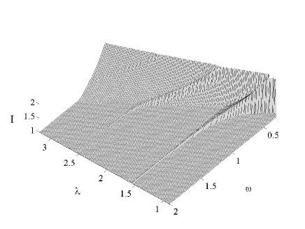
Figure 3: The scaled field intensity $I$ (20) as a function of $\lambda$ and $\omega$. Here the other dimensionless parameters are $\Omega=1$, $\Delta_{x}=2$ and $T=0.4$.

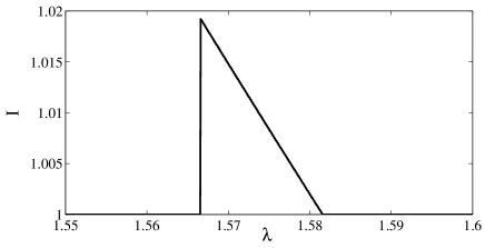
Figure 4: The scaled field intensity $I$ of the previous Fig. 2 (b) as function of $\lambda$ when fixing the field frequency $\omega=0.8$ and the width $\Delta_{x}=2$. This figure clearly demonstrates the presence of both first and second order QPTs.

Figures 3 and 4 characterize the type of QPT in the $\lambda-\omega$ phase diagram. The structure of the QPTs of the $T-\omega$ phase diagram turns out to be equally interesting. One example of the $T-\omega$ phase diagram is presented in Fig.5 (a). As for the $\lambda-\omega$ diagram, both first and second order QPT exist. Figure 5 (b), displaying the number of bound states, confirms that the sudden changes (first order QPTs) are due to additional bound states. The $T-\omega$ phase diagrams again display several different superradiant phases. In this case, however, there are both first and second order PTs between the superradiant phases. Interestingly, our numeric analysis indicates that the $T-\omega$ phase diagrams seem to be fairly independent of $\Omega$.

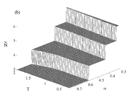
Figure 5: This figure displays in (a) the same as in Fig. 3, but for the $T-\omega$ plane (black curve of Fig. 2), while in (b) the number $\tilde{N}$ of bound states are shown. Note in (a) the large number of different suerradiant phases.

Contrary to the regular DM, in the ultracold regime atomic motion plays an important role for the system characteristics. The confining potential is determined for a given field intensity $y$, and consequently, the atomic density $\rho_{at}(x)$ per particle depends as well on $y$. In other words, apart from changes in the field intensity and in the atomic inversion, the phase transition will as wll be manifested in the atomic density. A natural consequence of the coupled system considered here is that the motional state of the atoms are entangled with the internal state. Thus, the phases (normal and superradiant) are intrinsically different from the ones of the regular DM. The regular DQPT derives from a competition between the free field energy and the interaction atom-field energy. While the free field is minimized by vacuum, the interaction energy decreases with an increasing field intensity. In the present model does the kinetic energy contribute to the total energy. It is thus an interplay between three terms; free field, atom-field interaction (containing the bare internal atomic energies), and motional energies. This is not so evident from the free energy per particle (19), where the kinetic energy is hidden in the second term. To illuminate the importance of the atomic motion we study the atomic inversion $W$ defined as the probability for a single atom to be in its excited state $|e\rangle$ minus the probability for it to be in the ground state $|g\rangle$. Once the adiabatic approximation has been imposed we are left with a single internal state; the lower adiabatic state $|-\rangle_{ad}=\sin\theta|e\rangle+\cos\theta|g\rangle$. In particular, the angle $\tan 2\theta=2g(\hat{x})\sqrt{\rho_{0}}\alpha/\Omega\sqrt{N}$ depends on the spatial coordinate and the inversion becomes

$$W\equiv\mathrm{Tr}\left[\hat{\sigma}_{z}\rho_{at}(x)\right]=\int dx\left(\sin^{2}\theta-\cos^{2}\theta\right)\rho_{at}(x).$$ (21)

The above equation clarifies that the atomic motion enters the problem in a non-trivial way. It also shows how the internal atomic properties are taken care of even though in the adiabatic approximation the system properties derives from a single internal state $|-\rangle_{ad}$. We have numerically verified the appearance of the PT in terms sudden changes in $\rho_{at}(x)$ (first order PT) or $\partial\rho_{at}(x)/\partial x$ (second order PT).

In deriving the phase diagrams, tight confinement of the atoms in two directions has been assumed. If only the longitudinal motion is frozen out, one regains an effective two dimensional problem whose eigenvalues are obtained from the Schrödinger equation with potential $V(x,y)=-\lambda\exp\left(-\frac{x^{2}+y^{2}}{\Delta_{x}^{2}}\right)$. As in the one dimensional situation studied in this section, $V(x,y)$ possesses a finite number of bound states and one would expect very similar phase diagrams for this two dimensional case as for the one dimensional model.

III.3 Validity of the adiabatic approximation

We conclude this section by analyzing the adiabatic approximation. By a simple rotation, the amplitudes $\alpha$ appearing in the single atom Hamiltonian (6) can be taken real. For real $\alpha$, the two last terms of $h(\alpha)$ is readily diagonalized by the unitary transformation ad

$$U=\left[\begin{array}[]{cc}\cos\theta&\sin\theta\\ -\sin\theta&\cos\theta\end{array}\right],$$ (22)

where the angle $\theta$ was given right above Eq. (21). Momentum transforms as $U\hat{p}U^{\dagger}=\hat{p}-\left(\hat{\sigma}^{+}+\hat{\sigma}^{-}\right)\partial\theta$, $\partial\theta\equiv\partial\theta/\partial\hat{x}$. Due to the spatial dependence of $\theta=\theta(\hat{x})$, the transformed Hamiltonian is non-diagonal; $\tilde{h}(\alpha)\equiv Uh(\alpha)U^{\dagger}=h_{ad}(|\alpha|)+h_{cor}(\alpha)$. Here, $h_{ad}(|\alpha|)$ is the adiabatic Hamiltonian (7) and $h_{cor}(\alpha)$ contains the non-adiabatic corrections. Explicitly one finds ad

$$h_{cor}(\alpha)=\frac{1}{2}\left[\begin{array}[]{cc}\left(\partial\theta\right)^{2}&2i\left(\partial\theta\right)\hat{p}+\partial^{2}\theta\\ -2i\left(\partial\theta\right)\hat{p}-\partial^{2}\theta&\left(\partial\theta\right)^{2}\end{array}\right].$$ (23)

The kinetic energy is smaller or of the same order as $\max_{x}V_{ad}^{+}(x,|\alpha|^{2})$, which provides a measure of $h_{cor}(\alpha)$ in comparison to the adiabatic Hamiltonian $h_{ad}(|\alpha|)$. For typical parameters, $\omega=\Omega=1$, $\Delta_{x}=3$, and $y=2$, the terms of $h_{cor}(\alpha)$ are at least one order of magnitude smaller than the terms of $h_{ad}(|\alpha|)$, which justifies the use of the adiabatic approximation.

IV Longitudinal thermodynamics

In the previous section we studied how the DQPT was modified due to motion of the atoms in a finite potential well, assuming the atomic motion to be frozen out in the longitudinal and one transverse direction. Here we instead assume the atoms to move freely along the center axis of the Fabry-Perot cavity while tightly bound in the transverse directions.

The corresponding single atom Hamiltonian (6) reads

$$h(\alpha)=\frac{\hat{p}^{2}}{2m}+\frac{\hbar\Omega}{2}\hat{\sigma}^{z}+\hbar\frac{\lambda\cos(\mu\hat{x})\sqrt{\rho_{0}}}{\sqrt{N}}\left(\alpha\hat{\sigma}^{+}+\alpha^{*}\hat{\sigma}^{-}\right),$$ (24)

where $\mu$ is the scaled photon wave number which will be set to unity hereafter, $\mu=1$. This Hamiltonian, with the field still quantized, has been considered in several papers, see for example effmass . Normally $L\gg 2\pi$, where $L$ is the cavity length, so neglecting boundary effects is not a crude approximation effmass . The Hamiltonian is of the form of a generalized Mathiue equation, and hence the spectrum $E_{\nu}(k)$ is described by a band index $\nu$ and a quasi momentum $k$ extending over the first Brillouin zone. Due to the internal two-level structure of the atom, the Brillouin zone is twice the size of what is imposed by the periodicity of the mode effmass . Clearly, $E_{\nu}(k)$ depends on the field amplitude $\alpha$. The corresponding eigenfunctions are written $\Phi_{k,\nu}(x)=\phi_{k,\nu}^{(e)}(x)|e\rangle+\phi_{k,\nu}^{(g)}|g\rangle$. For a constant coupling $g(x)=\lambda_{0}$, these Bloch functions are simple plane waves giving a constant energy shift independent of system parameters such as $\lambda$, $\omega$, and $\Omega$. For a standing wave mode coupling on the other hand, the Bloch functions cannot be decoupled from the internal atomic states, and consequently the atomic motion will affect the structure of the phase diagrams as will be demonstrated below.

In the previous section we assumed the adiabatic regime and diagonalized the Hamiltonian in its internal degrees of freedom. In this case, the adiabatic potentials $V_{ad}^{\pm}(x)$ cross and adiabaticity breaks down in the range where the QPTs occur. Fortunately, the Hamiltonian is easily diagonalized numerically by truncation the dimension of the Hamiltonian matrix. We present, however, asymptotic analytical results in the Appendix which relies on the adiabatic approximation. These analytical results enable us to extract the limiting situation of large field amplitudes. Furthermore, as a numerical diagonalization directly renders several of the Bloch bands we do not restrict the analysis to just the lowest one. However, it turns out that for most of the presented examples only the lowest band contribute to the dynamics due to the low temperatures considered. Exceptions are in the plots of the critical temperature where we indeed go to rather high temperatures and the excited bands become important.

The partition function is written like in the previous section as

$$Z=N\frac{C_{2}}{\sqrt{N}}\max_{0\leq y\leq\infty}\left\{\mathrm{e}^{Nf_{2}(y)}\right\},$$ (25)

where $C_{2}$ is a constant and the free energy per particle

$$f_{2}(y)=-\beta\hbar\omega y+\ln\left[g_{2}(y)\right]$$ (26)

with

$$g_{2}(y)=\sum_{\nu=1}^{\infty}\int_{-1}^{+1}dk\,\mathrm{e}^{-\beta E_{\nu}(k)}$$ (27)

Here, as above, $y=|\alpha|^{2}/N$ represent the scaled field intensity. Shown in the Appendix, the second part of $f_{2}(y)$ scales asymptotically as $\sim\sqrt{y}$ for large $y$. Thus, a maximum of the free energy can only be obtained for finite or zero field intensities $y$.

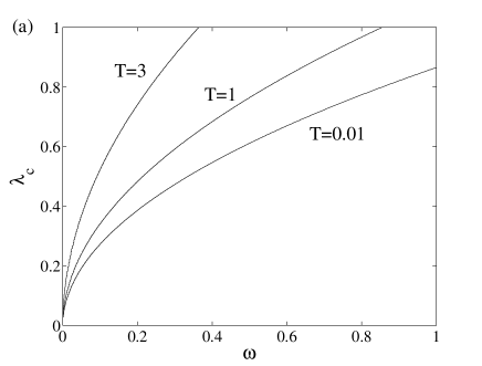
Figure 6: The dimensionless critical atom-field coupling $\lambda_{c}$ as function of $\omega$ (a) and $\Omega$ (b). In (a) $\Omega=1$ and in (b) $\omega=1$. The numbers to each curve display the dimensionless temperature $T$. Note in particular that for $\Omega\rightarrow 0$, the critical coupling $\lambda_{c}\neq 0$.

As in Sec. III, we derive the critical atom-field coupling $\lambda_{c}$ and temperature $T_{c}$. In Fig. 6 we show the results of how the critical coupling depends on $\omega$ (a) and $\Omega$ (b) for different temperatures. The critical temperature as function of $\omega$ and $\Omega$ is displayed in Fig. 7, where the inserted numbers indicate the values of the coupling $\lambda$. In both cases, the critical quantities show clear differences compared to the ones of the regular DM, (2). The critical coupling scales as $\lambda_{c}\sim\sqrt{\omega}$ for fixed $\Omega$ just like in the regular DM. However, the $\Omega$-dependence is not possessing the same structure as (2), and especially for small values on $\Omega$ the critical coupling $\lambda_{c}$ is non-zero. This was also found in a nearest-neighbor coupling model studied in onePT .

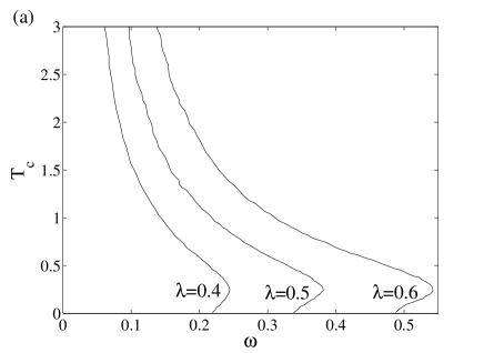
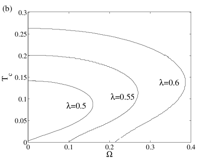
Figure 7: The dimensionless critical temperature $T_{c}$ as function of the system parameters. The inserted numbers give the value of $\lambda$. We note that a QPT is possible at zero temperature and finite $\omega$, and moreover, that for zero $\Omega$ the QPT may vanish for small temperatures. In (a) $\Omega=1$ while in (b) $\omega=1$.

In the regular DM, for a fixed $\lambda$ and $\Omega$ the critical temperature diverges for small $\omega$ and goes to zero for large $\omega$. Here we note that for high temperatures the regular behavior is regained, while for low temperatures, and in particular zero temperature, a QPT takes place for finite $\omega$. Fixing $\omega$ instead and vary $\Omega$ we get even more surprising results. In the regular DM, there is an upper temperature for which the QPT is lost and at zero temperature a QPT occurs for finite $\Omega$. In our model, a similar phase-diagram is obtained for a range of parameters $\omega$ and $\lambda$, but there also exist parameter regimes where no QPT occurs for zero temperature.

Like in the previous section the nature of the PTs is studied by introducing the scaled field intensity $I$ maximizing $f_{2}(y)$. It is found that the QPT’s are of second order character in all cases.

V Conclusions

In this work we have studied a new regime in the DM. The atoms are assumed trapped by the cavity field itself and ultracold such that their center-of-mass kinetic energy is of the order of the atom-field interaction. This calls for a full quantum mechanical treatment of the atomic motion and at the same time take into account for spatial mode variations. The analysis is motivated from our earlier findings, where we demonstrated that atomic motion greatly affects the system dynamics in many-body cavity QED systems jonas1 . Expectedly, we have shown that this is also true for the DM. The analysis is restricted to considering one dimensional problems, and both the case of a Gaussian and a standing wave mode profile were treated. However, we motivated that similar phenomena are expected also for higher dimensional situations. In particular, we made evident that the varying number of bound states in the potential formed by a Gaussian mode profile induces novel first order QPTs. Additionally, we found that for certain couplings $\lambda_{s}$, the system is superradiant for any field frequency $\omega$. Moreover, great differences with the regular DM was also encountered for a standing wave mode profile.

Appendix A Tight binding approach

Here, we analytically consider the large field asymptotic expressions for the energy per particle $f_{2}(y)$ in the case of a standing wave mode profile. In this regime one may utilize the tight binding approximation AM to derive the spectrum. We further assume the adiabatic approximation to be valid and that we can restrict the analysis to the lowest energy band. The adiabatic potentials are given by

$$V_{ad}^{\pm}(x)=\pm\hbar\sqrt{\frac{\Omega^{2}}{4}+\lambda^{2}\cos^{2}(x)y},$$ (28)

where $y=|\alpha|^{2}/N$ is as before the scaled field intensity. A convenient base for writing down the periodic Hamiltonian in matrix form is to use the Wannier states $w_{j}^{\pm}(x)=\langle x|j\rangle_{w,\pm}$ AM . The function $w_{j}^{\pm}(x)$ is localized in the $j$th ”well” of the potentials $V_{ad}^{\pm}(x)$. By the tight binding approximation we assume ${}_{w,\pm}\langle i|h_{ad}^{\pm}|j\rangle_{w,\pm}=0$ unless $i=j$ or $i=j\pm 1$. Within the validity regime of this approximation we may as well replace the Wannier functions by Gaussian functions jonas1 . The widths of the Gaussians are given by approximating the potential wells by harmonic oscillators, giving

$$w_{j}^{\pm}(x)\approx w_{G}^{\pm}(x-x_{j})\equiv\frac{1}{\sqrt[4]{\pi\sigma^{2}}}\mathrm{e}^{-\frac{(x-x_{j})^{2}}{2\sigma^{2}}},$$ (29)

where

$$\sigma^{2}=\left(\left.\frac{\partial^{2}V_{ad}^{\pm}(x)}{\partial x^{2}}\right|_{x=x_{j}}\right)^{-1}$$ (30)

and $x_{j}$ is the position of the $j$th potential well. To avoid un-physical contributions from the non-orthogonality of the Gaussians we impose $\int dx\,w_{G}(x-x_{j})w_{G}(x-x_{i})=\delta_{ij}$. We further introduce the matrix elements

$$\begin{array}[]{l}\displaystyle{E_{i}(y)\!=\!\int_{-\infty}^{\infty}\!dx\,{w_{G}^{\pm}}^{*}\!(x\!-\!x_{j})\!\left(\!-\frac{1}{2}\frac{\partial^{2}}{\partial x^{2}}\right)\!w_{G}^{\pm}(x\!-\!x_{j+i})}\\ \\ \displaystyle{J_{i}^{\pm}(y)\!=\!\int_{-\infty}^{\infty}\!dx\,{w_{G}^{\pm}}^{*}\!(x\!-\!x_{j})V_{ad}^{\pm}(x,|\alpha|^{2})w_{G}^{\pm}(x\!-\!x_{j+i})},\end{array}$$ (31)

where we only consider $i=0,1$. We note that the Wannier functions are directly related to the depth of the corresponding potential and therefore their width $\sigma$ will also depend on $y$. This explains the field intensity dependence of $E_{i}(y)$. Another important observation is that $w_{G}^{\pm}(x-x_{j})$ are localized where $|V_{ad}^{\pm}(x)|$ are close either to its maximum or its minimum, resulting in different coupling elements $J_{i}^{\pm}(y)$, indicated by the $\pm$-superscript. In this notation we get the lowest band tight binding energy

$$\begin{array}[]{lll}E_{1}^{\pm}(k)&=&E_{0}(y)+J_{0}^{\pm}(y)\\ \\ &&+\left[E_{1}(y)+J_{1}^{\pm}(y)\right]2\cos(k).\end{array}$$ (32)

The part in front of the cosine function is strictly negative resulting in that the ground state energy is given by $k=0$. The kinetic energy integrals of (31) are readily solvable, and one finds

$$\begin{array}[]{l}\displaystyle{E_{0}(y)=\frac{1}{4\sigma^{2}}},\\ \\ \displaystyle{E_{1}(y)=-\frac{1}{8\sigma^{4}}\exp\left(-\frac{\pi^{2}}{4\sigma^{2}}\right)\left(2\sigma^{2}+\pi^{2}\right)}.\end{array}$$ (33)

The potential integrals of (31) are not analytically solvable for the given potentials (28). Instead we make the same kind of approximation as in section III

$$V_{ad}^{\pm}(x)\approx\pm A\pm B\cos^{2}(x),$$ (34)

and identify

$$\begin{array}[]{l}\displaystyle{A=\frac{\Omega}{2}},\\ \\ \displaystyle{B=\sqrt{\frac{\Omega^{2}}{4}+\lambda^{2}y}-\frac{\Omega}{2}}.\end{array}$$ (35)

Within this regime we find

$$\begin{array}[]{l}\displaystyle{J_{0}^{\pm}(y)=\pm\frac{\Omega}{2}+\frac{1}{4\sqrt{m}\sigma^{2}}\left(1\mp\mathrm{e}^{-\sigma^{2}}\right)},\\ \\ \displaystyle{J_{1}^{\pm}(y)=\pm\frac{1}{4\sigma^{2}}\mathrm{e}^{-\frac{\pi^{2}}{4\sigma^{2}}}\mathrm{e}^{-\sigma^{2}}}.\end{array}$$ (36)

We emphasize that the width $\sigma^{2}$ depends on the field intensity $y$;

$$\sigma^{2}=\frac{1}{2B}.$$ (37)

The applied approximations are only reliable for $z<1$ jonas1 , and it turns out that the QPTs occur beyond these approximations. Nonetheless, we may find the asymptotics for the free energy $f_{2}(y)$. In the large $y$ limit we find that $\ln\left[g_{2}(y)\right]\sim\sqrt{y}$. Consequently, the field intensity $I$ will always be finite, regardless of parameter choices. We have verified numerically the $y$ square-root dependence of $\ln\left[g_{2}(y)\right]$ for large intensities.