Optimal Design and Optimal Control of Elastic Structures
Undergoing Finite Rotations and Elastic Deformations
A. Ibrahimbegović1, C. Knopf-Lenoir2,
A. Kučerová1 and P. Villon2
1Ecole Normale Supérieure - Cachan, LMT, GCE, 61, avenue du président Wilson,
94235 Cachan, France, email: ai@lmt.ens-cachan.fr
2Université de Technologie - Compiegne, Lab. Roberval, GSM,
60200 Compiegne, France
Abstract
In this work we deal with the optimal design and optimal control of structures undergoing large rotations. In other words, we show how to find the corresponding initial configuration and the corresponding set of multiple load parameters in order to recover a desired deformed configuration or some desirable features of the deformed configuration as specified more precisely by the objective or cost function. The model problem chosen to illustrate the proposed optimal design and optimal control methodologies is the one of geometrically exact beam. First, we present a non-standard formulation of the optimal design and optimal control problems, relying on the method of Lagrange multipliers in order to make the mechanics state variables independent from either design or control variables and thus provide the most general basis for developing the best possible solution procedure. Two different solution procedures are then explored, one based on the diffuse approximation of response function and gradient method and the other one based on genetic algorithm. A number of numerical examples are given in order to illustrate both the advantages and potential drawbacks of each of the presented procedures.
Keywords: structures, finite rotation, optimization, control
1 Introduction
Modern structures should often be designed to withstand very large displacements and rotations and remain fully operational. Moreover, the construction phase has also to be mastered and placed under control, with trying to precisely guide the large motion of a particular component of the total structural assembly. Ever increasing demands to achieve more economical design and construction thus require that the problems of this kind be placed on a sound theoretical and computational basis, such as the one explored in this work. Namely, optimization methods can be called upon to guide the design procedure and achieve desired reduction of mechanical and/or geometric properties. Similarly, the control methods are employed to provide an estimate of the loads and the minimal effort in placing the structure, or its component, directly into an optimal (desired) shape. Either of these tasks, optimal design or optimal control, can formally be presented as the minimization of the chosen cost or objective function specifying precisely the desired goal. The main difference between two procedures concerns the choice of the variables defining the cost function: the design variables are typically related to the mechanical properties (e.g. Young’s modulus) or geometry of the structure (e.g. particular coordinates in the initial configuration), whereas the control variables are related to the actions (e.g. forces) applied on the structure in order to place it into desired position. Rather then insisting upon this difference and treating the optimal design and optimal control in quite different manners (as done in a number of traditional expositions on the subject), we focus in this work on their common features which allow a unified presentation of these two problems and the development of a novel solution procedure applicable to both problems. The latter implies that the nonlinear mechanics model under consideration of geometrically exact beam has to be placed on the central stage and one should show how to fully master the variation in chosen system properties or loads in order to achieve the optimal goal. The main contributions put forward in presenting this unconventional approach can be stated as follows:
-
i)
We first present the theoretical framework for treating nonlinear structural mechanics and optimization and/or control as a coupled (nonlinear) problem; In any such problem of optimization or control, the nonlinear mechanics equilibrium equations are reduced to a mere constraint with respect to the admissibility of a given state of the structure, i.e. its displacements and rotations. By using the classical method of Lagrange multipliers (e.g. see [19] or [29] the mechanics equilibrium equations can be promoted from constraint to a one the governing equations to be solved in a coupled problem of this kind, and the intrinsic dependence on state variables (displacements and rotations) with respect to optimal design or control variables can be eliminated turning all variables into the independent variables. For clarity, this idea is also developed within the framework of a discrete, finite-element-based approximation, thus providing the finite element model including the degrees of freedom pertinent not only to displacements and rotations, but also to optimal design and/or control variables. A detailed development is presented for the chosen model problem of 3D geometrically exact beam (e.g. see [27] or [10]). We note in passing that the proposed approach is quite opposite from the traditional ones (e.g. see [17] for a very recent review), where the two fields directly concerned by the coupled problems of this kind, nonlinear mechanics on one side and optimal design or control on the other, are studied and developed separately and resulting solution procedures for one or another are applied in a sequential manner. One typically employs two different computer programs, one for mechanics and another for optimization or control (e.g. the toolbox of MATLAB), so that the communication requirements are reduced to a bear minimum: so-called sensitivity (e.g. [30] or [25]) for optimization code, and design or control variables for the finite element code for mechanics. It is clear that such a traditional approach to analysis and design or control will largely sacrifice the computational efficiency for the cases of practical interest where both the cost function and mechanics problem are nonlinear and require iterative procedures to be solved.
-
ii)
The second aspects which is elaborated upon in this work pertains to an alternative method for solving a coupled problem for analysis and either design or control, where two sub-problems, once brought up to the same level by the Lagrange multiplier method, are solved simultaneously. In other words, once the interdependence of the state variables, i.e. the displacements and rotations on one side and the design or control variables or another, is no longer enforced, one can iterate simultaneously to solve for all of them. In particular, the sensitivity analysis needs no longer be performed separately, but it is naturally integrated as a part of the simultaneous iterative procedure. It is important to note that the iterative intermediate values are no longer consistent with the equilibrium equations constraint, except at the convergence, where basically the same solution is obtained as for the standard sequential solution procedure but with a (significantly) reduced number of iterations. In other words the simultaneous and sequential solution procedures will always yield the same result providing the solution is unique. The problems of this kind concern the optimization and/or control of geometrically nonlinear response of structures where no bifurcation phenomena occur. Solving the nonlinear problems in structural mechanics can be quite a demanding task for the structures where the stiffness may differ significantly in different deformation modes (i.e. beam bending versus stretching). Adding the control or optimization problem on top makes such a nonlinear problem so much more challenging. Different modifications of the basic solution procedure are developed and tested, including genetic algorithms [7] to explore the initial phase of the solution procedure, gradient based acceleration near solution points and response surface for a part of the solution constructed by diffuse approximation (e.g. see [2]).
The outline of the paper is as follows. In the next section we briefly present the chosen model of geometrically exact 3D beam, capable of representing very large displacements and rotations. The theoretical formulation of the optimal control and optimal design of the chosen mechanical model is presented in Section 3, along with their discrete approximations constructed by the finite element method given in Section 4. The proposed solution procedure is described in detail in Section 5. Several numerical examples are presented in Section 6 in order to illustrate the performance of various algorithms used in computations. Some closing remarks are stated in Section 8.
2 Model problem: geometrically exact 3D beam
In this section, we briefly review the governing equations of the chosen model problem of a structure undergoing large rotations, a 3D curved beam. For a more thorough discussion of the chosen model we refer to [27], [26] or [13], among others. We assume that the initial configuration of the beam is internal force free and that it can be described by a 3D position vector (s) identifying the position of each point of the neutral fiber (an inextensible fiber in pure bending) and the corresponding placement of the cross-section of the rod, which is carried out by choosing a local ortho-normal triad of vectors. The vector triad of this kind can be obtained by simply rotating the global triad by an orthogonal tensor.For a usual choice of so-called normal coordinates with the first vector of the triad being orthogonal to the cross-section and the remaining two placed in the plane of the cross section, this orthogonal tensor becomes a known function of the initial configuration, . For the case of a curved beam studied here, ’’ is chosen as the arc length parameter.
By applying the external loading , parameterized by pseudo-time ’t’ (where ’pseudo’ implies that the inertia effects are neglected) we obtain the beam deformed configuration defined by the position vector and the orthogonal tensor . The latter is an accordance with the usual kinematic hypothesis that the cross-section of the beam would not deform, which, along with the hypothesis that the first vector in the triad remains orthogonal to it (with other two within the plane of the cross-section) fully determines . See Figure 1 where the initial and deformed configuration of the beam are presented.
In short, one can state that the configuration space of the described model of 3D beam can be written as
| (1) |
where and are spaces of 3D vectors and special orthogonal tensors, respectively.
The main difficulty in numerical solution of the structural mechanics problems featuring the beams of this kind stems from the presence of group in its configuration space (e.g. see [1], [13], [11] for a more thorough discussion of these issues). In short, in performing the standard task of computing the virtual work principle or the consistent linearization, where a small rotation described by a skew-symmetric tensor , ought to be superposed on a large rotation described by an orthogonal tensor one must first make use of exponential mapping
| (2) |
where is the axial vector of the skew-symmetric tensor i.e. .
The complexity of the last expression is in sharp contrast, with respect to a simple additive update of virtual displacement field when superposed on the deformed configuration
| (3) |
The results in (2) and (3) can be presented in an equivalent form by stating that the tangent space of the chosen beam model is defined by
| (4) |
The strain measures employed in this beam theory (e.g. [10]) can be written in direct tensor notation form as
| (5) |
for the axial and shear strains, and
| (6) |
for bending and torsional strains. In (5), (6) and subsequent equations we denote with superposed prime the derivative with respect to arc-length coordinate in the initial configuration, i.e.
| (7) |
We consider the simplest case of linear elastic material model for the beam which allows us to express the constitutive equations in terms of stress resultants as
| (8) |
| (9) |
For illustration, we also consider the simplest case of a circular cross section, with section diameter ’’, and
| (10) |
as the section area, moment of inertia and polar moment.
In order to complete the description of the chosen beam model we state the equilibrium equations in the weak form as
| (11) |
where is the external virtual work and and are the virtual strains. The latter can be obtained as the Gâteaux derivative of the real strains in (5) and (6), by taking the results in (2) and (3) into consideration. In particular, this leads to
and
which can also be written in an equivalent form in terms of the corresponding axial vectors
| (14) |
For the external load which derives from a given potential, such that
| (15) |
one can also define the governing equilibrium equation of the chosen model problem of the geometrically exact elastic beam from the principle of minimum of the total potential energy defined according to
| (16) |
which implies that
| (17) |
In (17) above we denoted by K the second variation of the total potential energy or the tangent operator, which is obtained by the consistent linearization procedure (e.g. see [20]). For pertinent details of the consistent linearization we refer to [10] for quaternion parameterization of finite rotations or [13] for rotation vector-like parameters for finite rotations.
An alternative case of external loading where the potential may not be defined and where the weak form in (11) is rather the starting point of the solution procedure, can also be encountered in applications. For example, in the case of the follower force and follower moment which follow the motion of a particular cross-section of the beam at node ’’, we can express their contribution to virtual work according to
| (18) |
The follower force and moment will also contribute to the tangent operator according to
| (19) |
where . This contribution should also be taken into account when computing the solution to (11) and trying to ensure the quadratic convergence rate.
3 Coupled optimality problem
The presented beam model provides an excellent basis to master the optimization problem as well as the control problem of geometrically nonlinear elastic structures. Although the former deals with geometric characteristics of the beam and the latter with the external loading sequence, the two problems can be formulated and solved in quite an equivalent manner, as shown next.
3.1 Optimal design
The optimal design problem addressed herein pertains to selecting the desired features of the mechanical model by leaving the free choice of the geometric properties of the beam model, e.g. the thickness variation or the chosen initial shape. This task is often referred to as the shape optimization. From the mathematical standpoint the shape optimization can be formulated as the problem of minimization of so-called objective or cost function , specifying the desired features. The latter is considered as a functional which depends not only on mechanics state variables but also on design variables (e.g. the beam thickness or its shape).
The shape optimization procedure is interpreted herein as minimization of so-called cost or objective functional ), which can be written as
| (20) |
Contrary to the minimization of the total potential energy functional in (17), not all mechanical and design variables are admissible candidates, but only those for which the weak form of the equilibrium equations is satisfied. In other words, we now need to deal with a constrained minimization problem.
The classical shape optimization procedure of solving this constrained minimization problem is carried out in a sequential manner, where for each iterative value of design variables , a new iterative procedure must be completed leading to verifying the equilibrium equations. The considerable computational cost of such a procedure, most of it waisted on iterating to convergence on equilibrium equations even for non-converged values of design variables, can be drastically reduced by formulating the minimization problem in (20) using the method of Lagrange multipliers with
| (21) |
In (21) above are the Lagrange multipliers inserted into the weak form of equilibrium equations instead of virtual displacements and rotations. In accordance to the results presented in the previous section we can write explicitly
| (22) |
The main difference of (21) with respect to constrained minimization problem in (20) pertains to the fact that state variables and design variables are now considered independent and they can be iterated upon (and solved for) simultaneously.
The Kuhn-Tucker optimality condition (e.g. [19]) associated with the minimization problem in (18) can be written as
| (23) |
with the explicit form of the last term which can be written as
| (24) |
where we denoted , as well as and , ; Moreover, we have
| (25) |
where
| (26) |
Finally, we also have
| (27) |
For illustration we can consider further that the diameter of a circular cross-section is chosen as the design variable, which allows us to express explicitly the result in (23) as
| (28) | ||||
| (29) |
In order to provide a similar explicit result for directional derivative of the cost function, we consider a simple choice given as the beam mass (or equivalently its volume for a constant density),
| (30) |
In such a case the contribution of the cost function to the Kuhn-Tucker optimality conditions can be written as
| (31) | ||||
We can also consider a more complex case of practical interest where the shape optimization is carried out with respect to the beam axis form in the initial configuration. A reference configuration is selected in such a case (see Figure 1) and the design variable is given in terms of the position vector describing the beam initial configuration with respect to this reference configuration . The cost function in (25) can now be described as
| (32) |
In this case all the integrals in (23) to (27) must be recomputed with the same change of variables like the one presented in (32) above typical of the isoparametric parent element mapping (e.g. see Zienkiewicz and Taylor [31]). We also note in passing that the derivatives with respect to arc-length coordinate ought to be computed by making use of the chain rule
| (33) |
For example, the contribution of the cost function to the Kuhn-Tucker optimality conditions for such a choice of design variables can be written as
| (34) |
3.2 Optimal control
The optimal control problem studied herein concerns the quasi-static external loading sequence which is chosen to bring the structure directly towards an optimal or desired final state, which may involve large displacements and rotations. More precisely, we study the mechanics problems where introducing the pseudo-time parameter ’t’ to describe a particular loading program is not enough and one also needs to employ the control variables . The latter contributes towards the work of external forces, which can be written as
| (35) |
where contains the (fixed) distribution of the external loading to be scaled by the chosen control.
Optimal control can be presented in the following form: find the value of the control variables , such that the final value of the state variables be as close as possible to the desired optimal (fixed) values ; This can be formulated in terms of the constrained minimization of the chosen cost function which can be written as
| (36) |
where the role of the constraint, as indicated by the last expression, is to fix the values of the state variables with respect to the chosen value of the control through the given set of equilibrium equations. In other words, for a given control we will finally obtain the configuration the same as the desired state if the latter verifies equilibrium equations, or, in the opposite case simply the solution closest to which also verifies the equilibrium equations.
In order to remove this constraint and to be able to consider the state variables independently from the control variables, we resort to the classical method of Lagrange multipliers; Namely, by introducing the Lagrange multipliers we can rewrite the optimal control problem by making use of the Lagrangian functional which allows to obtain the corresponding form of the unconstrained optimization problem.
| (37) |
One can readily obtain the Kuhn-Tucker optimality conditions for this problem according to
| (38) | |||||
| (39) |
and
| (40) |
The first of these equations is precisely the weak form of equilibrium equation, whereas the second two will provide the basis for computing the control and the Lagrange multipliers . The explicit form of the equilibrium equation is similar to the one in (11) only with the external load term (35), but with the variation of the Lagrange multiplier replacing the virtual displacement . For writing the explicit form of other two Kuhn-Tucker equations we choose a particular form of the objective function such that
| (41) |
where is the desired beam shape and is a scalar parameter specifying the weighted contribution of the chosen control. With such a choice we seek to minimize the ”distance” between the desired shape and the computed admissible shape (the one which satisfies equilibrium) as well as the force or control needed to achieve that state. The explicit form of the first term in (39) and (40) can thus be written as
| (42) |
and
| (43) |
Explicit result for the second term of Kuhn-Tucker equations in (39) is identical to the one in (24) potentially modified according to (19) for the case of the follower load. Finally, the second term of the Kuhn-Tucker equation in (40) can be written as
| (44) |
which concludes with the description of all the problem ingredients.
4 Finite element discrete approximations
In this section we discuss several important aspects of numerical implementation of the presented theory for analysis and design and related issues which arise in numerical simulations.
The analysis part of the problem, i.e. the state variables are represented by using the standard isoparametric finite element approximations (e.g. see [31]). In particular, this implies that the element initial configuration is represented with respect to its parent element placed in the natural coordinate space, corresponding to a fixed interval, , by using
| (45) |
In (45) above is the position vector field with respect to the reference configuration, are nodal values of an element with nodes and are the corresponding shape functions. The latter can easily be constructed for beams by using the Lagrange polynomials, which for an element with nodes can be written by using the product of monomial expressions
| (46) |
where , are the nodal values of natural coordinates.
With isoparametric interpolations one chooses the same shape functions in order to approximate the element displacement field, which allows us to construct the finite element representation of the element deformed configuration as
| (47) |
where are the nodal values of the position vector in the deformed configuration. The virtual and incremental displacement field are also represented by isoparametric finite element interpolations
| (48) |
The latter enables that a new (iterative) guess for the deformed configuration be easily obtained with the corresponding additive updates of the nodal values
The finite element approximation of the incremental displacement field in (48) above, where at each point the corresponding value is a linear combination of the nodal values, are referred to as the continuum consistent (e.g. see [9, 10]), since they allow to commute the finite element interpolation and the consistent linearization of nonlinear problem (e.g. [20]). Therefore, we also choose the isoparametric interpolations for virtual and incremental rotation field with
| (49) |
so that the commutativity of the finite element discretization and consistent linearization would also apply to the rotational state variables. The only difference from the displacement field concerns the multiplicative updates of the rotation parameters, which can be written for any nodal point as
| (50) |
In the combined analysis and design procedure proposed herein one must also interpolate the Lagrange multipliers, which is also done by using the isoparametric interpolations according to
| (51) |
The corresponding integrals appearing in governing Lagrangian functional in (21) or Kuhn-Tucker optimality conditions in (23), (25) and (27) are computed by numerical integration (e.g. Gauss quadrature, see [31]). To illustrate these ideas we further state a single element contribution to the analysis part of the governing Lagrangian functional in (22) given in the discrete approximation setting by
| (52) |
where and are the abscissas and weights of the chosen numerical integration rule (e.g. see [31]) and is the total number of integration points for a single element.
In order to complete the discretization procedure one must also specify the interpolations of the design variables. If the latter is the thickness or the diameter for the chosen case of a circular cross-section, or the element nodal coordinates, it is possible to use again the isoparametric finite element approximations. However, the best results are obtained by reducing the number of design variables as opposed to those chosen at the element level, by using the concept of a design element. This implies increasing the degree of polynomial by employing, for example, Bézier and B-spline curves for representation of beam shape and reducing significantly the number of design parameters (e.g. see [16] for a detailed discussion of these ideas). What is important to note from the standpoint of the simultaneous solution procedure presented further on is that the design variable at any point is given as a linear combination of the design element interpolation parameters
| (53) |
Consequently, the finite or rather design element discretization and consistent linearization will commute again. This observation was already made earlier for linear analysis problem by Chenais and Knopf-Lenoir [3]. With these results on hand we can write the discrete approximation of equilibrium equations as
| (61) | |||||
where ’A’ denotes the finite element assembly operator.
By the same token the discrete approximation of the Kuhn-Tucker optimality conditions in (23) can be presented as
| (80) | |||||
Similarly, for the simple choice of the objective function in (30) the discrete approximation of the optimality condition in (25) can be written as
| (88) | |||||
In summary, the discrete approximation of the optimal design problem reduces to the following set of nonlinear algebraic equations where the unknowns are the nodal values of displacements and rotations, the corresponding values of Lagrange multipliers and the chosen values of thickness parameters which support Bézier curve thickness interpolations,
| (89) |
Similar procedure leads to the discrete approximation of the optimal control problem. In fact, the first of the nonlinear algebraic equations in (54) is only slightly modified to include the control variables in accordance with the expression in (35)
| (90) |
where are the chosen control parameters.
For the particular choice of the objective function of the control problem given in (41), we can further obtain the discrete approximation of the optimality condition in (39) according to
| (91) |
The discrete approximation of the last optimality condition in (40) can also be written explicitly as
| (92) |
We note in passing that the last two optimality conditions can be combined to eliminate the Lagrange multipliers leading to
| (93) |
The last result can be combined with the equilibrium equations in (90) providing a reduced set of equations with nodal displacements, rotations and control variables as the only unknowns. This kind of form is fully equivalent to the arc-length solution procedure, which is used for solving the nonlinear mechanics problems in the presence of the critical points (e.g. see [24], [4] or [23], among others). One can recognize that (90) is only a particular choice of the supplementary condition which is used to stabilize the system.
5 Solution procedure
Two novel solution procedures are developed for solving this class of problems of optimal design and optimal control as described next.
5.1 Diffuse approximation based gradient methods
The first solution procedure is a sequential one, where one first computes grid values of the cost function and then carry out the optimization procedure by employing the approximate values interpolated from the grid. It is important to note that all the grid values provide the design or control variables along with the corresponding mechanical state variables of displacements and rotations which must satisfy the weak form of equilibrium equation. In other to ensure this requirement, for any grid value of design or control variables one also has to solve associated nonlinear problem in structural mechanics.
The main goal of the subsequent procedure is to avoid solving these nonlinear mechanics problems for other but grid values, and simply assume that the interpolated values of the cost function will be ”sufficiently” admissible with respect to satisfying the equilibrium equations. Having relaxed the equilibrium admissibility requirements we can pick any convenient approximation of the cost function, which will simplify the subsequent computation of the optimal value and thus make it much more efficient. These interpolated values of the cost function can be visualized as a surface (yet referred to as the response surface) trying to approximate sufficiently well the true cost function. The particular method which is used to construct the response surface of this kind is the method of diffuse approximations (see [22] or [2]). By employing the diffuse approximations the approximate value of the cost function is constructed as the following quadratic form
| (94) |
where is a constant reference value, is the gradient and is the Hessian of the approximate cost function. In (94) above variables should be replaced by either design variables for the case of an optimal design problem or by control variables in the case when we deal with an optimal control problem.
We further elaborate on this idea for a simple case where only 2 design or control variables are used, such that . For computational proposes in such a case one uses the polynomial approximation typical of diffuse approximation (see [2]) employing the chosen quadratic polynomial basis and a particular point dependent coefficient values
| (95) |
By comparing the last two expressions one can easily conclude that
| (96) |
The approximation of this kind is further fitted to the known, grid values of the cost function; , trying to achieve that the point-dependent coefficients remain smooth when passing from one sub-domain to another. This can be stated as the following minimization problem:
| (97) |
where are the weighting functions associated with a particular data point , which are constructed by using a window function based on cubic splines according to
| (98) |
with for the present 2-component case) as the closest grid nodes of the given point . We can see that the weighting functions in (97) and (98) above take a unit value at any of the closest grid nodes and vanish outside the given domain of influence. While the former assures the continuity of the coefficients , the latter ensures that the approximation remains local in character. Similar construction can be carried out for higher order problems, which requires an increased number of closest neighbors in the list.
By keeping the chosen point fixed and considering the coefficients of diffuse approximation as constants, the minimization of amounts to using the pseudo-derivative of diffuse approximation (see [22]) in order to compute yielding the minimum of according to
| (99) |
which allows us to write a set of linear equations
| (100) | |||
We note in passing that the computed minimum value of does not necessarily provide the minimum of the true cost function, which also has to satisfy the equilibrium equations; however, for a number of applications this solution can be quite acceptable. If the latter is not sufficient, we ought explore an alternative solution procedure capable of providing the rigorously admissible value of any computed minima of the cost function, by carrying out the simultaneous solution of the cost function minimization and the equilibrium equations. The proposed procedure is based on genetic algorithm as described next.
5.2 Genetic algorithm based method
Genetic algorithms belong to the most popular optimization methods nowadays. They follow up an analogy of processes that run in nature within the evolution of living organisms over a period of many millions of years. Unlike the classic gradient optimization methods, genetic algorithms operate on so called population which is a set of possible solutions, applying the genetic operators, such as cross-over, mutation and selection. The principles of genetic algorithm was first proposed by Holland [6]. Ever since, the genetic algorithms have reached wide application domain (e.g. see the books of Goldberg [5] and Michalewicz [21] for extensive review).
Genetic algorithms in the original form operate on population of so-called chromosomes. These are binary strings which represent possible solutions in a certain way. In engineering problems we are usually working with real variables, which in the kind of applications described further are optimized values of load control or design variables. Adaptation of the genetic algorithm idea to this problem is made possible by Storn [28] by considering the chromosomes as vectors instead of binary strings and using differential operators which can affect the distance between the chromosomes.
In this work we employ an improved version of this kind of algorithm referred to as ’Simplified Atavistic Differential Evolution’, or SADE ([18]). It is shown [7, 8] that the algorithm is well suitable for dealing with a fairly large number of variables which is of particular interest for the problem on hands. The SADE algorithm is designed to explore all possible minima and thus find the global minimum, even for the case where the cost function may have very steep gradients and isolated peak values. Only a short description of the corresponding procedure is given subsequently (see [7] for a more elaborate presentation).
In the tradition of evolutionary methods, the first step is to generate a starting generation of chromosomes by choosing the random values of all state variables along with those for control or design. Subsequently we repeat until convergence the cycles containing: the creation of a new generation of chromosomes, by mutation, local mutation or cross-over and the evaluation and selection, which reduces the actual number of chromosomes to the initial number.
In the computations to follow we will work with the population of ’’ chromosomes, where ’’ is the total number of unknowns in the problem. This population can evolve through the following operations; Mutation: let be the i-th chromosome in a generation g,
| (101) |
where is the number of variables of the cost function. If a certain chromosome is chosen to be mutated, a random chromosome is generated from function domain and a new one is computed using the following relation:
| (102) |
Parameter is the constant of algorithm equal to . Number
of new chromosomes created by the operator ’mutation’ is defined
by ’radioactivity’, which is another parameter of the algorithm,
with a constant value set to for all our calculations. If a
certain chromosome is chosen to be locally mutated, all its
coordinates have to be altered by a random value from a given
(usually very small) range. Its aim is to utilize the near
neighborhood of existing chromosomes and make search for improved
solutions faster. It is useful only for cost functions with steep
gradients in the case, where near the optimal function value, a
small change in value of variable may introduce a large change in
function value. The aim of the cross operator is to create as many
new chromosomes as there were in the last generation. The operator
creates new chromosome according to the following
sequential scheme: choose randomly two chromosomes
and , compute their difference vector, multiply it
by a coefficient CR and add it to the third, also randomly
selected chromosome , i.e,
| (103) |
Every component exceeding the defined interval is changed to the appropriate boundary value of domain. The parameter has probably the most important effect on the algorithm’s behavior; it seems that if the speed up of the convergence is needed, this parameter should be set to some lower value (from to ). In the opposite case, the higher values of this parameter could improve the ability to solve for any local minimum. In our computations this value was set to .
Selection represents the kernel of the genetics algorithm. The goal is to provide a progressive improvement of the whole population, which is achieved by reducing the number of ”living” chromosomes together with conservation of better ones. Modified tournament strategy is used for this purpose: two chromosomes are chosen randomly from a population, they are compared and the worse of them is cast off. This conserves population diversity thanks to a good chance of survival even for badly performing chromosomes.
It was observed that the SADE algorithm can be quite inefficient in the later stage of the analysis, where the solution with all or a large number of components is almost converged. For that reason we have tried to further improve the performance by forcing the algorithm to stick better to these converged values. In particular we have experimented with a modified form of the cross operator, which contrary to the one in (103) will produce the new chromosome by building on top of the best possible previous value according to
| (104) |
where is the sign change parameter which is supposed to get the correct orientation of the increase with respect to the gradient. Moreover, the parameter is no more constant, but its values are chosen randomly from interval , where is new parameter of the algorithm, with a smaller influence at its behavior than . Operator local mutation is now switched off and parameter in operator mutation is also no more constant, but chosen randomly from interval . This algorithm modification is subsequently referred to as GRADE.
6 Numerical examples
In this section we present several illustrative examples dealing with the coupled problems of mechanics and either optimal control or optimal design. The computations are carried out by using a mechanics model of 2D geometrically exact beam (see [12] or [14]) developed either within the MATLAB environment for diffuse approximation based solution procedure or within the SADE computer code for genetic algorithms.
6.1 Optimal control of a cantilever structure in the form of letter T
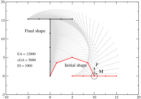
In this example we study the optimal control problem of deploying initially curved cantilever beam in the final configuration which takes the form of letter T. See Figure 2 for initial and final configurations indicated by thick lines and a number of intermediate deformed configurations indicated by thin lines. The chosen geometric and material properties are as follows: The diameter of the circular curved part and the length of the flat part of the cantilever are both equal to ; the beam cross-section is a unit square; the chosen values of Young’s and shear moduli are and , respectively.
The deployment is carried out by applying a vertical force and a moment at the end of the curved part of the cantilever. In other words the chosen control is represented by a vector . The desired shape of the cantilever which takes the form of letter T corresponds to the values of force and moment . The optimal control problem is then defined as follows. The objective or cost function is defined by imposing the desired shape only on displacement degrees of freedom with
| (105) |
which is further recast in the discrete approximation setting as
| (106) |
where are computed and are desired nodal displacements. We note in passing that no condition is imposed through the cost function on either rotational degrees of freedom or control vector, which nevertheless introduces no difficulties in solving this problem.
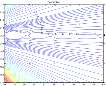
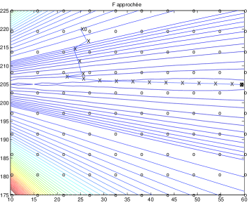
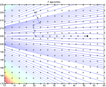
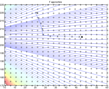
The first solution is obtained by the diffuse approximation based gradient method. The calculation of the cost function is first carried out for all the ’nodes’ of the following grids: . The gradient type procedure is then started on the grid and, thanks to the smoothness of the diffuse approximation base representation of the approximate value of the cost function, converged with no difficulty in roughly 20-40 iterations. The iterative values obtained in the gradient method computations are for different grids shown in Figure 3. Grid is constructed for the following interval of values of force and moment:
|
 |
|---|---|
| Grid () | Grid () |
| Solution : | Solution : |
| 38 evaluations of AD | 38 evaluations of AD |
|
 |
| Grid () | Grid () |
| Solution : | Solution : |
| 19 evaluations of AD | 15 evaluations of AD |
We note that all different choices of the grid can result in different solutions, since none of the solutions of this kind will satisfy the equilibrium equations.
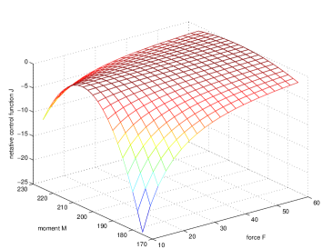
Quite large difference between known optimal solution and solutions of response surface could be explained by different influence of each control variable to value of cost function, see Figure 4. All used grids weren’t able to describe small influence of force .
 |
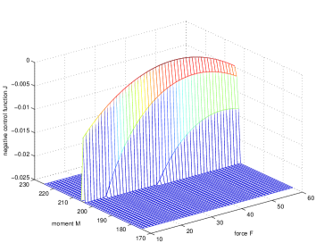 |
| Whole scale of values. | More detailed about value of optimum. |
The second solution method used for this problem employs the genetic algorithm based computation. In this computation we have used the same admissible intervals like in the previous case for the control variables, force and moment. The computations are carried out starting from the random values chosen in this interval and stopped when the first value of the cost function is found.
In order to be able to look into statistics, one hundred runs are performed with each one converging to the exact solution. Three types of procedures were tried, with either tuning on or off the parameters controlling local mutation (LM) and the gradient-type acceleration of sign change (SG). The results are presented in Table 1.
| Letter T problem | |||
|---|---|---|---|
| Computation | Number of fitness calls | ||
| with SADE | Minimum | Maximum | Mean Value |
| LM-on SG-off | 240 | 2860 | 648.8 |
| LM-off SG-off | 280 | 1680 | 625.4 |
| LM-off SG-on | 220 | 1640 | 591.2 |
We can see that the best performance is achieved with the simple gradient-like modification of SADE genetic algorithm to accelerate convergence in the latest stage. The results obtained with this simple gradient-like modification of SADE algorithm can further be improved by using described GRADE algorithm, with a special role of the radioactivity parameter. See Table 2.
| Letter T problem | |||
|---|---|---|---|
| Computation | Number of fitness calls | ||
| with GRADE | Minimum | Maximum | Mean Value |
| radioactivity = 0.0 | 180 | 880 | 410.0 |
| radioactivity = 0.1 | 240 | 1200 | 440.8 |
| radioactivity = 0.2 | 280 | 1180 | 512.4 |
| radioactivity = 0.3 | 280 | 1300 | 588.4 |
The second solution procedure applied to the same example is so-called simultaneous solution of mechanics equilibrium and optimal control equations, written explicitly in (90) to (92) with value . The total numb er of unknowns in this case is equal to 44, with 2 control variables (the force and the moment), 21 components of nodal displacements and rotations and 21 Lagrange multiplier. For computational convenience, the problem of solving the set of nonlinear algebraic equations in (90) to (92) is recast as the minimization statement which allows direct application of the genetic algorithm with
| (107) |
The solution efficiency of the proposed simultaneous procedure depends on the chosen upper and lower bounds of the admissible interval and the initial guess for the solution. For example, the mechanics state variables are chosen as these featuring in the desired beam shape, , and the bounds are controlled by the chosen parameter according to
| (108) |
The equivalent bounds on control variables are obtained from the precious result obtained by solving the grid minimization problem which results with the minimum of the response surface. Finally, the Lagrange multipliers is solved for from (91) where the adopted values for and are chosen.
One hundred computations is performed with the indicated bounds on the unknowns. Value of parameter is set to . Choice of parameters of GRADE algorithm were: and ’radioactivity’ equal to . Table 3 summarizes the statistics of this computation.
| Minimum | Maximum | Mean Value | Standard deviation | |
| 39.957 | 40.048 | 40.000 | 0.0199 | |
| 204.86 | 205.15 | 205.00 | 0.0548 | |
| number of evaluations of | 100740 | 298080 | 172176 | ——— |
The last part of the analysis carried out in this examples concerns an attempt to further increase the efficiency of the simultaneous solution procedure. In that sense, we employ the GRADE version of genetic algorithm with the choice of parameters and ’radioactivity’ equal to . A very small value of bounds is chosen as well with . The computations we have performed with a hundred runs of the genetic algorithm can be summarized with the statistics given in Table 4.
| Minimal | Maximal | Mean Value | Standard deviation | |
| 39.973 | 40.034 | 40.000 | 0.0135 | |
| 204.96 | 205.05 | 205.00 | 0.0192 | |
| number of evaluations of | 14720 | 201480 | 37701 | ——— |
We can see from Table 4 that the proper choice of the bounds can force the algorithm to always converge to the same solution. The latter is the consequence of using the simultaneous solution procedure which assures that the computed solution also satisfies the equilibrium equations. Moreover, the total cost of the simultaneous solution procedure can be reduced beyond the one needed for response-surface-based approximate solution computations, by either reducing the interval as done herein or by making gradient-type modification of this algorithm in order to accelerate the convergence rate.
6.2 Optimal control of a cantilever structure in form of letter I
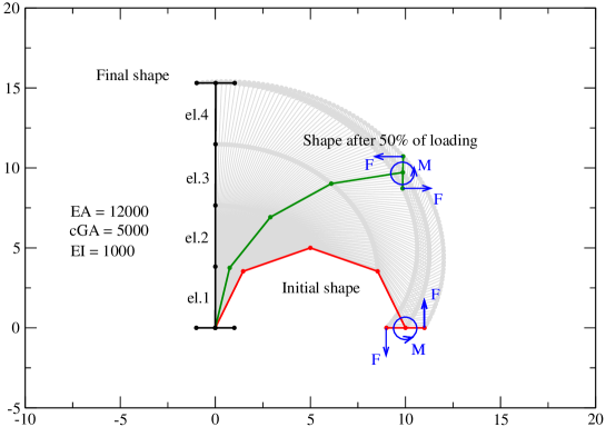
In the second example we deal with a problem which has a multiple solution and its regularized form which should restore the solution uniqueness. To that end, a cantilever beam is used very much similar to the one studied in the previous example, except for a shorter straight bar with length equal . The cantilever is controlled by a moment and a couple of follower forces which follow the rotation of the cross-sections to which they are attached. The initial and final configuration, which is obtained for a zero couple and a moment are shown in Figure 5, along with a number of intermediate configurations.
The first computation is performed with the cost function identical to the one in (106), imposing only the minimum of difference between the desired and the computed deformed shape, with no restriction on control variables. The computation is carried out by using the GRADE genetic algorithm by starting with random values within the selected admissible intervals for the force couple and moment according to
The algorithm performance is illustrated in Table 5.
| Letter I problem | ||
| Number of fitness calls | ||
| Minimum | Maximum | Mean Value |
| 180 | 640 | 359.8 |
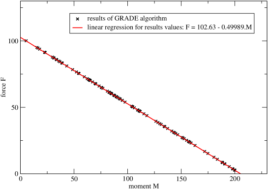
A number of different solutions have been obtained with different computer runs which were performed (see Figure 6). However, all these solutions remain in fact clearly related considering that the applied moment and the force couple play an equivalent role in controlling the final deformed shape; It can be shown for this particular problem that any values of force and moment which satisfy a slightly perturbed version (because of the straight bar flexibility) of the force equilibrium
will be admissible solution, thus we have infinitely many solutions for the case where only the final shape is controlled by the choice of the cost function.
In order to eliminate this kind of problem we can perform a regularization of the cost function, by requiring not only that the difference between computed and final shape be minimized but also that control variables be as small as possible; Namely, with a modified form of the cost function
| (109) |
where is a chosen weighting parameter specifying the contribution of the control. We set a very small value and choose the convergence tolerance to and carry out the computation for yet a hundred times. Whereas a more stringent value of the tolerance requires somewhat larger number of cost function evaluation, the result in each of the runs remains always the same, given as
and the found optimal value of the cost function is .
| Letter I problem extended | ||
| Number of fitness calls | ||
| Minimum | Maximum | Mean Value |
| 820 | 16320 | 1758.8 |
6.3 Optimal control of deployment of a multibody system
The optimal control procedure of the deployment problem of a multibody system is studied in this example. In its initial configuration the multibody system consists of two flexible component (with , and ) each 5 units long connected by the revolute joints (see [15]) to a single stiff component (with , and ) of the length equal to , which are all placed parallel to horizontal axis. In the final deployed configuration the multibody system should take the form of a letter B with the stiff component being completely vertical and two flexible component considerably bent. The deployment of the system is controlled by five control variables, three moments , and , a vertical and a horizontal force . See Figure 7.
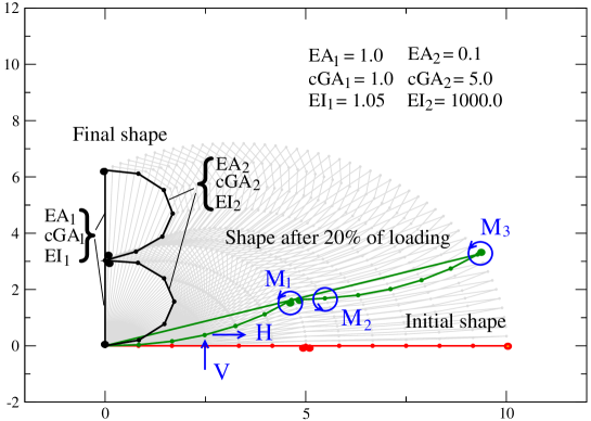
The cost function in this problem is again chosen as the one in 106, which controls that the system would find the configuration as close as possible to the desired configuration. The desired configuration of the system corresponds to the values of forces , and moments , and . The solution is computed by using the SADE and GRADE genetics algorithms and starting with the random choice in the interval of interest defined as
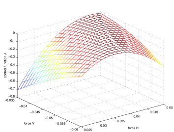
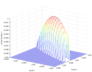
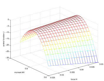
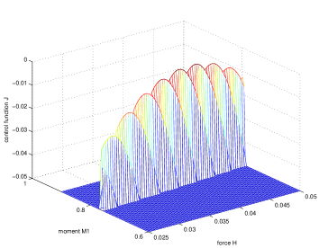
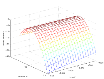
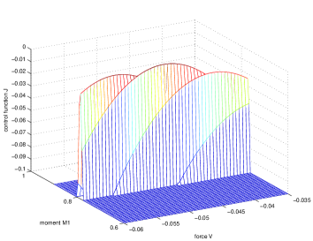
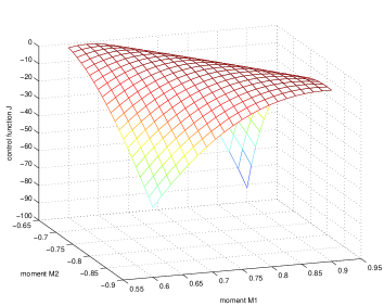
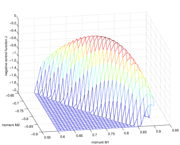
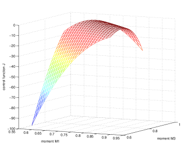
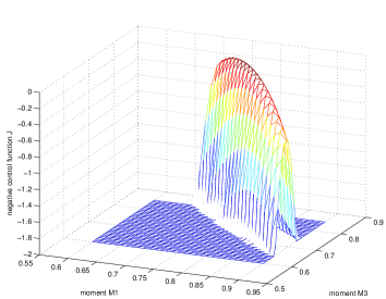
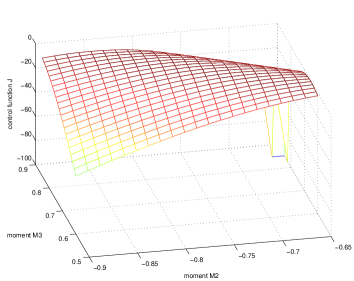
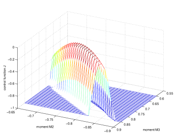
The solution of the problem is typically more difficult to obtain with an increase in the number of control variables, one of the reasons being a more irregular form of the cost function. In that sense,we refer to illustrative representation of the cost function contours in different subspaces of control variables as shown in Figures 8 and 9.
 |
 |
| subspace | subspace |
 |
 |
| subspace | subspace |
 |
 |
| subspace | subspace |
 |
 |
| subspace | subspace |
 |
 |
| subspace | subspace |
 |
 |
| subspace | subspace |
The convergence tolerance on cost function is chosen equal to . The SADE algorithm performance for the simplest choice of algorithm parameters is presented in Table 7 and the GRADE algorithm performance for modified value of radioactivity parameter is presented in Table 8.
| Letter B problem | |||
|---|---|---|---|
| Computation | Number of fitness calls | ||
| with SADE | Minimum | Maximum | Mean Value |
| LM-on SG-off | 2600 | 165800 | 46887.5 |
| LM-off SG-off | 2350 | 177150 | 42494.0 |
| LM-off SG-on | 2400 | 177850 | 34612.1 |
| Letter B problem | |||
|---|---|---|---|
| Computation | Number of fitness calls | ||
| with GRADE | Minimum | Maximum | Mean Value |
| radioactivity = 0.0 | —– | —– | —– |
| radioactivity = 0.1 | 1500 | 114050 | 23862.5 |
| radioactivity = 0.2 | 1900 | 117850 | 20632.0 |
| radioactivity = 0.3 | 3050 | 122550 | 34520.0 |
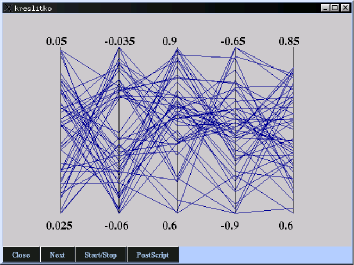
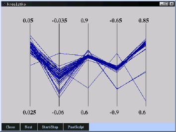
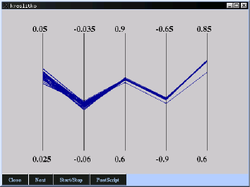
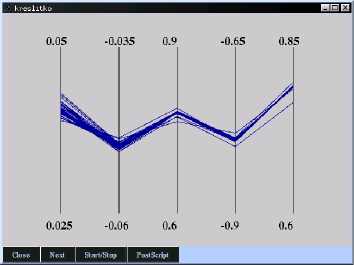
One can notice the order of magnitude of increase in cost function evaluation, which is brought about by a more elaborate form of the cost function (see Figures 8 and 9). However, the latter is not the only reason. In this particular problem the role of moments in the list of control variables is much more important than the role of the horizontal and vertical forces in bringing the system in the desired shape. This affects the conditioning of the equations to be solved and the slow convergence rate of the complete system is in reality only the slow convergence of a single or a couple of control components. The latter is illustrated in Figure 10, where we provide the graphic representation of iterative values for computed chromosomes, where every chromosome is represented by a continuous line. We can note that the population of optimal values of moments converges much more quickly than the force values which seek a large number of iteration in order to stabilize. Another point worthy of further exploration is the best way to accelerate the convergence rate in the final computational phase.
 |
 |
| G1:J=0.0091823 | G4:J=0.0071823 |
 |
 |
| G26:J=1.3302e-05 | G43:J=1.1839e-05 |
6.4 Optimal design of shear deformable cantilever
In this last example we study an optimal design problem which considers the thickness optimization of a shear deformable cantilever beam, shown in Figure 11.
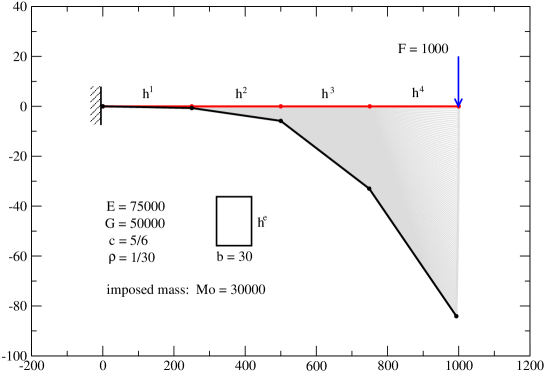
The beam axis in the initial configuration of the cantilever and the thickness is considered as the variable to be chosen in order to assure the optimal design specified by a cost function. In the setting of discrete approximation, we choose 4 beam elements each with a constant thickness , which results with 4 design variables . The beam mechanical and geometric properties are: Young’s modulus , shear modulus , rectangular cross section with width and mass density . The latter is needed for computing the total mass of the beam to be used as the corresponding limitation on the computed solution assuring reasonable values of the optimal thickness under the free-end vertical force . In order to assure a meaningful result the computations are performed under chosen value of mass limitation is . Other limitations are also placed on the admissible values of the thickness for each element.
The first computation is performed by using the diffuse approximation based response function and the sequential solution procedure. The cost function is selected as the shear energy of the beam and problem is cast as maximization of the shear energy, with
| (110) |
where is the shear strain component. The bounds on thickness values are chosen as shown in Table 9.
| Thickness | ||||
|---|---|---|---|---|
| Min | 30 | 30 | 15 | 15 |
| Max | 60 | 60 | 35 | 35 |
The diffuse approximation computations on the grid are started from an initial guesses for thickness . It took 11 iterations to converge to solution given as
The corresponding value of shear energy for this solution is ; we recall it is only an approximate solution, since the computed value does not correspond to any of the grid nodes.
The same solution is next sought by using GRADE algorithm; The chosen values for GRADE parameters are: , and ’radioactivity’. The genetic algorithm is executed 100 times, leading to the computational statistics reported in Table 10.
| Minimum | Maximum | Mean Value | |
|---|---|---|---|
| nb. of comput. | 120 | 3400 | 674.8 |
The algorithm yielded two different solutions, both essentially imposed by the chosen bounds; Namely, out of 100 runs, 57 converged to , with the corresponding value of , whereas 43 settled for with a very close value of . Hence, each of two solutions leads to an improved value of the cost function.
The second part of this example is a slightly modified version of the first one, in the sense that the mechanics part of the problem is kept the same and only a new cost function is defined seeking to minimize the Euclidean norm of the computed displacement vector, i.e.
| (111) |
Such a choice of the cost function is made for being well known to result with a well-conditioned system expressing optimality conditions. Indeed, the same type of sequential solution procedure using diffuse approximation of cost function now needs only a few iterations to find the converged solution, starting from a number initial guesses. The final solution value is given as
.
In the final stage of this computation we recompute the solution of this problem by using the genetic algorithm. The admissible value of the last element thickness is also slightly modified by reducing the lower bound to 5 (instead of 15) and higher bound to 25 (instead of 35) in order to avoid the optimal value which is restricted by a bound. The first solution to this problem is obtained by using again the sequential procedure, where the GRADE genetic algorithm is employed at the last stage. The computed value of the displacement vector norm for found solution is and mass is . The computations are carried out a hundred times starting from random initial values. The statistics of these computations are given in Table 11.
| Minimum | Maximum | Mean Value | Standard deviation | |
| 43.772 | 43.807 | 43.790 | 0.0094 | |
| 35.914 | 35.949 | 35.932 | 0.0088 | |
| 26.313 | 26.346 | 26.328 | 0.0082 | |
| 14.184 | 14.210 | 14.197 | 0.0064 | |
| nb. of comput. | 1440 | 9960 | 3497 | ——– |
The same kind of problem is now repeated by using the simultaneous solution procedure, where all the optimality condition are treated as equal and solved simultaneously resulting with 4 thickness variables, 15 displacement and rotation components and as many Lagrange multipliers as unknowns. The latter, in fact, is eliminated prior to solution by making use of optimality condition in (89. The chosen upper and lower bounds of the admissible interval are chosen as
| (112) |
where the guess for the displacement is obtained by solving mechanics problem with the values of thickness parameters given in Table 11. The limitation on total mass is added to the cost function. The choice of GRADE algorithm parameters is given as and ’radioactivity’ equal to . The computation is stopped with a fairly loose tolerance, which allows to accelerate the algorithm convergence but does not always lead a unique solution. Yet, the results in Table 12 show that standard deviation indeed remains small, or that the solution is practically unique.
| Minimum | Maximum | Mean Value | Standard deviation | |
| 43.782 | 43.794 | 43.789 | 0.0026 | |
| 35.925 | 35.935 | 35.930 | 0.0021 | |
| 26.315 | 26.324 | 26.319 | 0.0019 | |
| 14.197 | 14.202 | 14.200 | 0.0010 | |
| nb. of comput. | 111340 | 968240 | 313006 | ——– |
7 Acknowledgements
This work was supported by the French Ministry of Research and the European Student Exchange Program ERASMUS. This support is gratefully acknowledged.
8 Conclusions
The approach advocated herein for dealing with a coupled problem of nonlinear structural mechanics and optimal design or optimal control, which implies bringing all the optimality conditions at the same level and treating all variables as independent rather than considering equilibrium equations as a mere constraint and state variables as dependent on design or control variables, is fairly unorthodox and rather unexplored. For a number of applications the proposed approach can have a great potential. In particular, the problems of interest to this work concern the large displacements and rotations of a structural systems. The key ingredient of such an approach pertains to geometrically exact formulation of a nonlinear structural mechanics problem, which makes dealing with nonlinearity description or devising the solution schemes much easier then for any other model of this kind. The model problem of the geometrically exact beam explored in detail herein is not the only one available in this classl; We refer to work in [9] for shells or to [10] for 3D solids, with both models sharing the same configuration space for mechanics variables as 3D beam. The latter also allows to directly exploit the presented formulation and the solution procedures of a coupled problem of nonlinear mechanics, for either shells or 3D solids, and optimal control or optimal design.
Two different solution procedures are presented herein; the first one, which exploits the response surface representation of the true cost function followed by a gradient type solution step, leads to only an approximate solution. Although the quality of such a solution can always be improved by further refining the grid which serves to construct the response surface, the exact solution is never computed unless the minimum corresponds to one of the grid points. The second solution procedure, which solves simultaneously the optimality conditions and nonlinear mechanics equilibrium equations, does deliver the exact solution, although often only after the appropriate care is taken to choose the sufficiently close initial guess and to select the admissible intervals of all variables accordingly. Probably the best method in that sense is the combination of sequential and simultaneous procedure, where the first serves to reduce as much as possible the admissible interval and provide the best initial guess, whereas the second furnishes the exact solution.
A number of further improvements can be made for the proposed methods of this kind, to help increase both the convergence rates and accuracy of the computed solution. One has to remember that even only mechanics component equilibrium equations for a problem of this kind can be very difficult to solve, since the large difference in stiffness in different modes (e.g. bending versus stretching) can result with a poorly conditioned set of equations. Adding the optimality conditions on top only further increases the difficulty. Finding the best possible way to deal with this problem is certainly worthy of further explorations.
References
- [1] J.H. Argyris. An excursion into large rotations. Comput. Methods Appl. Mech. Eng., 32:85–155, 1982.
- [2] P. Breitkopf, C. Knopf-Lenoir, A. Rasineux, and P. Villon. Efficient optimization strategy using hermite diffuse approximation. In H. Mang, editor, Proceedings Fifth WCCM, Vienna, 2002.
- [3] D. Chenais and C. Knopf-Lenoir. From design sensitivity to code structure in arch optimization. In Opti 89, Southampton, U.K.
- [4] M. A. Crisfield. A fast incremental/iterative solution procedure that handles snap through. Computers & Structures, 13:55–62, 1981.
- [5] D.E. Goldberg. Genetic algorithms in search, optimization and machine learning. Addison-Wesley, 1989.
- [6] J. H. Holland. Adaptation in natural and artificial systems. University of Michigan, Ann Arbor, MI, Internal report, 1975.
- [7] O. Hrstka and A. Kučerová. Improvements of the different types of binary and real coded genetic algorithms preventing the premature convergence. Advances in Engineering Software in press, 2003.
- [8] O. Hrstka, A. Kučerová, M. Lepš, and J. Zeman. A competitive comparison of different types of evolutionary algorithms. Computers and Structures, 81/18-19:1979–1990, 2003.
- [9] A. Ibrahimbegović. Stress resultant geometrically nonlinear shell theory with drilling rotations - part 1: a consistent formulation. Comput. Methods Appl. Mech.Eng., 118:265–284, 1994.
- [10] A. Ibrahimbegović. Finite element implementation of reissner’s geometrically nonlinear beam theory: three dimensional curved beam finite elements. Comput. Methods Appl. Eng., 122:10–26, 1995.
- [11] A. Ibrahimbegović. On the choice of finite rotation parameters. Comput. Methods Appl. Mech. Engng., 149:49–71, 1997.
- [12] A. Ibrahimbegović and F. Frey. Finite element analysis of linear and non-linear planar deformations of elastic initially curved beams. International Journal for Numerical Methods in Engineering, 36:3239–3258, 1993.
- [13] A. Ibrahimbegović, F. Frey, and I. Kozar. Computational aspects of vector-like parameterization of three-dimensional finite rotations. International Journal for Numerical Methods in Engineering, 38:3653–3673, 1995.
- [14] A. Ibrahimbegović and S. Mamouri. Nonlinear dynamics of flexible beams in planar motions formulation and time-stopping scheme for stiff problems. Comp. Struct., 70:1–22, 1999.
- [15] A. Ibrahimbegović and S. Mamouri. On rigid components and joint constraints in nonlinear dynamics of flexible multibody systems imployin 3d geometrically exact beam model. Comp. Methods Appl. Mech. Eng., 188:805–831, 2000.
- [16] M. Kegl. Shape optimal design of structures: an efficient shape representation concept. Int. J. Numer. Meth. Engng., 49:1571–1588, 2000.
- [17] M. Kleiber, H. Antunez, T.D. Hein, and P. Kowalczyk. Parameter sensitivity in nonlinear mechanics; theory and finite element computations. John Wiley & Sons, 1997.
-
[18]
A. Kučerová and O. Hrstka.
Homepage of SADE.
http://klobouk.fsv.cvut.cz/ondra/sade/sade.html. - [19] D.G. Luenberger. Linear and nonlinear programming. Addison-Wesley Publ., 1984.
- [20] J.E. Marsden and T.J.R. Hughes. Mathematical foundations of elasticity. Prentice-Hall, 1983.
- [21] Z. Michalewicz. Genetic Algorithms+Data Structures=Evolution Programs. Springer-Verlag, 1992.
- [22] B. Nayroles, G. Touzot, and P. Villon. Generalizing the finite element method: diffuse approximation and diffuse elements. Computational Mechanics, 10:307–318, 2002.
- [23] E. Ramm. Strategies for tracing the non-linear response near limit points. In W. Wunderlich, editor, Nonlinear Finite Element Analysis in Structural Mechanics, pages 63–89, Berlin, 1988. Springer-Verlag.
- [24] E. Riks. The application of newton s method to the problem of elastic stability. Journal of Applied Mechanics, 39:1060–1066, 1972.
- [25] B. Rousselet. A finite strain rod model and its design sensitivity. Mechanics of Structures and Machines, 20:415–432, 1992.
- [26] J.C. Simo. The (symmetric) hessian for geometrically nonlinear models in solid mechanics: intrinsic definition and geometric interpretation. Comput. Methods Appl. Mech. Engng., 96:183–200, 1992.
- [27] J.C. Simo and L. Vu-Quoc. Three-dimensional finite strain model - part ii: computational aspects. Comput. Methods Appl. Mech. Eng., 38:79–116, 1986.
- [28] R. Storn. On the usage of differential evolution for function optimization. In Biennial Conference of the North American Fuzzy Information Processing Society, pages 519–523, 1996.
- [29] G. Strang. Introduction to applied mathematics. Wellesley-Cambridge Press, 1986.
- [30] D.A. Tortorelli and P. Michaleris. Design sensitivity analysis: overview and review. Inverse Problems in Engineering, 1:71–105, 1994.
- [31] O.C. Zienkiewicz and R.L. Taylor. The finite element method, volume vols I, II & III. Butterworth, London, 2000.