SU-ITP-09/06
SLAC-PUB-13536
Trapped Inflation
Daniel Greena, Bart Horna, Leonardo Senatoreb,c and Eva Silversteina
a SLAC and Department of Physics, Stanford University,
Stanford CA 94305, USA
b School of Natural Sciences, Institute for Advanced Study,
Olden Lane, Princeton, NJ 08540, USA
c Jefferson Physical Laboratory and Center for Astrophysics, Harvard University, Cambridge, MA 02138, USA
Abstract
We analyze a distinctive mechanism for inflation in which particle
production slows down a scalar field on a steep potential, and show
how it descends from angular moduli in string compactifications. The analysis of density perturbations – taking into account the integrated effect of the produced particles and their quantum fluctuations – requires
somewhat new techniques that we develop. We then
determine the conditions for this effect to produce sixty
e-foldings of inflation with the correct amplitude of density
perturbations at the Gaussian level, and show that these
requirements can be straightforwardly satisfied. Finally, we estimate the amplitude of the non-Gaussianity in the power spectrum and find a significant equilateral contribution.
1 Introduction
Inflation [1] is a very general framework for addressing the basic problems of primordial cosmology. It requires a source of stress-energy which generates an extended period of accelerated expansion. This can arise in many different ways even at the level of a single scalar inflaton, for which the space of inflationary models has been usefully organized by an effective field theory treatment [2]. The various mechanisms can be distinguished in many cases via their distinct predictions for the CMB power spectrum and for relics such as cosmic strings that may be produced after inflation. As well as being observationally accessible, inflationary theory is also sensitive to the ultraviolet completion of gravity, for which string theory is a promising candidate.
Traditional slow roll inflation requires a flat potential, which can be obtained naturally using approximate shift symmetries or with modest fine-tuning. Inflation, however, does not require a flat potential. Rather, in general in single-field inflation [2, 3] the inflaton may self-interact in such a way as to slow itself down even on a steep potential as in e.g. [4, 5, 6, 7]. It is interesting to examine such mechanisms further, to explore their novel dynamics and to better assess the level of fine-tuning required to obtain them from the point of view of both effective field theory and string theory.
In this work, we analyze a simple mechanism for inflation in which the inflaton rolls slowly down a steep potential by dumping its kinetic energy into the production of other particles (plus appropriate supersymmetric partners) to which it couples via interactions of the form
| (1.1) |
As rolls past each point , the corresponding particles become light and are produced with a number density that grows with increasing field velocity . As it dumps energy into the produced particles, slows down; meanwhile the produced particles dilute because of the Hubble expansion. With sufficiently closely spaced points we will see that this yields inflation even on a potential that is too steep for slow-roll inflation. This mechanism, trapped inflation, was originally suggested in [8] based on the preheating mechanism developed by [9] 111There are other interesting approaches using a gas of particles to slow the field evolution on a steep potential in order to inflate (see e.g. the recent review [10] and [11]) or to avoid the overshoot problem in small-field inflationary models (see e.g. [12, 13, 14]). The change in the CMB power spectrum from a single particle production event was also studied in [15].. It can be usefully viewed [5] as a weak-coupling analogue of DBI inflation (or vice versa) in which the effects on ’s motion from the production of the fields dominates over their loop corrections to its effective action.
From the low energy point of view, although couplings of the general form (1.1) are generic, the prospect of many closely spaced such points seems rather contrived. However, we will see that just this structure descends from string compactifications in a rather simple way. It arises in the same type of angular directions in field space that undergo monodromy from wrapped branes as studied recently in [16, 17].
In [16, 17], a single wrapped brane was considered. A scalar rolls down the potential over a large distance corresponding to multiple circuits of an underlying circle around which the brane tension undergoes monodromy. In this super-Planckian regime, the potential satisfies slow roll conditions as in chaotic inflation [18] (though with a distinctive power law behavior depending on the example). In the same direction, at sub-Planckian field values , the potential is too steep for slow roll inflation. However, in variants of these setups, because of the underlying small circle, the system periodically develops new light degrees of freedom as the inflaton rolls down the steep part of the potential.
The analysis of the perturbation spectrum in this class of models, including the integrated effects of the produced particles, has interesting novelties. The number of produced particles fluctuates quantum mechanically, leading to a source term in the equation of motion for the perturbations of the inflaton. A constant solution to the homogeneous mode equation develops parametrically before the mode stretches to the Hubble horizon, as in previous examples of single field inflation in the presence of a low sound speed [3, 19, 6]. Finally, as with other mechanisms such as [5, 6] in which interactions slow the inflaton, a simple estimate reveals a correspondingly large non-Gaussian contribution to the perturbation spectrum in trapped inflation, which will be within the range tested by the upcoming Planck satellite [20] according to preliminary estimates for its capacity to detect or constrain the three-point amplitude
While this work was in completion we received the interesting work [21], which has some overlap with the present paper.
2 Background Solution
In this section we will find the background solutions and the conditions for trapped inflation, without making use of the perturbation spectrum. We will discuss perturbations in the next section. Getting the power spectrum to match observation will further constrain our parameters.
The idea of trapped inflation is that particle production will slow the inflaton () enough to produce inflation on a potential which would be too steep for slow-roll inflation. For this to work, we will need a number of different fields to become massless at regular intervals along the direction. A Langrangian describing such a configuration can be written as
| (2.2) |
where the represent the supersymmetric completion of these terms, applicable in appropriate cases. Softly broken supersymmetry helps to suppress Coleman-Weinberg corrections to the effective action arising from the loops of light particles. As discussed in [5, 8], at weak coupling particle production dominates over quantum corrections to the effective action for colliding locally maximally supersymmetric branes. Here the points are the points where become massless. For simplicity, we take these to be evenly spaced in with spacing . The coupling may be small. If starts rolling down the potential , whenever it crosses a point , particles are produced. The expectation value 222For the purposes of calculating the homogeneous background inflationary solution, the expectation value of is all we will need. In calculating the perturbation spectrum in the next section, we will require its higher point correlation functions. of the number density of the particles produced is given by [9, 8]
| (2.3) |
where is defined by and the powers accounts for the dilution of particles due to the expansion of the universe. The energy density of the particles is then given by following the particle production event, i.e. once the system has passed back into the adiabatic regime where . Because , the fields behave adiabatically when
| (2.4) |
Making the replacement , we can estimate the timescale on which the particle production happens: . Requiring this timescale to be short compared to Hubble implies
| (2.5) |
The parametric dependence of eq. (2.3) can be understood by noticing that the particle are effectively massless at production time, and are produced during a time of order . This explains why . On a longer timescale, Hubble dilution becomes important, and .
The equations for motion for the homogeneous background solution (including the energy density in particles) can be derived either from or by approximating with in the equations of motion for as explained in [9]. The equation of motion is
| (2.6) |
where . This sum over particle production events will be difficult to deal with, so we would like to replace it with an integral, giving us
| (2.7) |
This is a good approximation to the sum when the variation of the integrand is small between production events. This is quantified by the two conditions and . Because of the exponential suppression and the slow variation of the integrand, we can replace the integral by
| (2.8) |
This is a reasonable approximation under the condition . If we assume slow roll and that the particle production is the dominant mechanism for damping (), then we can solve (2.7) to get
| (2.9) |
It is worth commenting on the limit of the above expression. In this case goes to zero. This is due to the fact that in absence of dilution, the mass of the particles increases as moves after the time of particle-production. Therefore, loses energy even after the particles stop being produced. This explains why, in this limit, the solution is different from the const. that one would naively expect in the case of a linear potential. In the presence of a non-zero , the growth in mass of the particles is compensated by their dilution, which allows for a steady solution const. to exist.
Given the solution for in eq. (2.9), we can find and the slow roll parameters. The usual Friedmann equation is
| (2.10) |
We are assuming that the energy density is dominated by the potential energy. Using energy conservation we get
| (2.11) |
where we have used . The generalized slow roll parameter is then given by
| (2.12) |
As expected is the statement that the energy density is dominated by the potential.
We would like to use to constrain our parameters. We will assume that so our condition becomes
| (2.13) |
In order to constrain our parameters, we will make some estimates of this integral. Using (given ), we can do the integral to get
| (2.14) |
Using (2.9), and dropping order one factors 333In general, we will not keep track of all order one factors, in part because our analysis of the integro-differential equation governing and its perturbations will not be exact., we get
| (2.15) |
We are now in a position to massage some of our previous inequalities to get conditions on individual parameters. Using (2.5), we can use our solution to get the inequality
| (2.16) |
This provides a lower bound on . The requirement that the particle production events were frequent also gave us the inequality . Using (2.9), this gives us
| (2.17) |
These two inequalities imply
| (2.18) |
We can also use our constraints on to get analogues of the slow-roll condition . Recall that our solution required . Taking a derivative of (2.9) we get
| (2.19) |
The first inequality, is trivially satisfied for the first term, but the second gives us a new condition
| (2.20) |
The second inequality, also gives a non-trivial condition
| (2.21) |
There is another important requirement that we have ignored. Inflation is required to last long enough to give at least 60 e-folds. We will discuss this constraint in the context of an model, after we discuss perturbations.
3 Perturbations
3.1 Gaussian Perturbations
Determining the form of the curvature perturbation is a delicate task. Since the trapping is intrinsically a multifield effect, we have not developed a Langrangian description of our effective equation of motion for that one can consistently perturb. The strategy that we will use instead is to study the perturbations using the equations of motion directly.
There are two approaches one could take. The first is to use constant , ‘unitary’, gauge and perturb in the metric. This would seem to have an obvious advantage, given that the particle production would happen everywhere at the same time in this slicing. Unfortunately, solving the many constraint equations for the metric perturbation is a complicated task. Similarly to what occurs in spontaneously broken gauge theories when one works in unitary gauge, this would also be the gauge where the main physical degrees of freedom are most obscure. As is usually the case in inflation [2], the matter scalar degree of freedom produces some scalar perturbations on the metric. These are not independent scalar degrees of freedom, but they are constrained variables. These perturbations of the metric are less important than the matter scalar excitations (the scalar field and the particles in our case) for all the range of energies that we are interested in: from deep inside the horizon to freezeout. Thus, it is convenient to work in a gauge where the scalar field and the particles appear explicitly, so that one can neglect the metric perturbations. This leads us to the second possible approach to study the perturbations, which will be the one we take here, where we work with constant curvature slices. In reality, since metric perturbations are less important, we will forget about them from the start, and we will work directly in an unperturbed quasi de Sitter universe. We will therefore perturb our equation of motion for , taking into account the variance in the number density of fields created. After horizon exit, at the time of reheating, these are converted to the curvature perturbation in the standard way [22].
The equation of motion for takes the form
| (3.22) |
We have assumed as before that we can make the sum of sets of produced particles into an integral (an approximation to be checked below), and we have included their quantum fluctuations in the last term.
In the Gaussian approximation, the last term in (3.22) is equivalent to the variance in the number of produced particles:
| (3.23) |
This behaves as a source term in the equation for the inflaton perturbations. This is somewhat analogous to the equation for perturbations discussed in [23], and we can use some of the same techniques. We will now perturb the field around the background solution as
| (3.24) |
When expanding our equation of motion in , we have to be careful to keep all the contributing terms. In particular, fluctuations of the inflaton change the time when particle production occurs at different spatial points. This manifests itself as a fluctuation of , our variable of integration, when we use the continuum approximation to the sum over particle production events. We define by . Expanding in and , we find
| (3.25) |
We should think of the integral as being over . This implies that the upper limit of the integral is also subject to the perturbation. In particular, we can think of the integral as being over all time with a step function . This accounts for the fact that, on equal time slices, at different spatial locations, a different number of fields could have become massless and therefore been produced. In these regions, a different number of particles contribute to the sum, leading to a different region of integration.
Putting these pieces all together we get the equation of motion for the fluctuation
| (3.26) |
where we have done a Fourier transform in the spatial direction with being the physical momentum. For the Gaussian fluctuations, we will expand to linear order in . This gives an effective equation of motion
| (3.27) |
where we have defined and used (3.23). One can check that is the -like condition (2.20), so we will drop the term. We will see that this condition, not , is sufficient to ensure that the spacetime is accelerating, and the modes freeze-out and produce curvature perturbations. This is very different than in the standard slow-roll case.
There are two types of contributions to the power spectrum – those sourced by , and those which would arise in the absence of the source. We will find that the former dominates. To begin, in order to analyze both these contributions, we require the homogeneous mode solutions to the above integro-differential equation. This will allow us to construct the Green’s function required to determine the sourced perturbations.
To get some intuition for the behavior of the homogenous solutions, we will start by solving the equation for constant . This is a good approximation when which holds until . We will also approximate and as constant, which holds to leading order in our generalized slow roll parameters. There are three epochs of interest depending on the ratios and :
(I) : The modes are approximately Minkowskian, with both Hubble friction and particle production effects negligible in their equations of motion; we start with the pure positive frequency modes corresponding to the standard Bunch-Davies vacuum.
(II) : In this regime, a constant solution to (3.27) appears. The mode solutions from region I, evolved into region II, develop a term which is approximately constant. This contribution begins with a very small amplitude (which will be determined in our exact solution below) but ultimately dominates over the other terms which become damped exponentially in .
(III) : In this regime, the curvature perturbation becomes constant, lying outside the Hubble horizon.
In particular, we will find that the modes actually freeze-out well before reaching the Hubble horizon. This is somewhat analogous to the freeze-out of modes at the sound horizon in general single field models of inflation [4, 19, 6, 5].
Now let us derive these features from a more detailed analysis of (3.27). For constant , and , we can find exact solutions to (3.27) using the ansatz . We can solve the equation trivially because in our WKB regime of constant , all terms are proportional to with constant coefficients depending on and . In particular, using the ansatz and doing the integrals we find that (3.27) reduces to
| (3.28) |
This equation gives the mode solutions when . Multiplying through by , we get the cubic equation
| (3.29) |
where we have defined . It should be clear from this equation that behavior of the perturbations will only be different from the usual case if . In this model, this is always the case, as this condition is equivalent to the slow roll condition .
There are three analytic solutions to (3.29) since it is a cubic. To understand the behavior of the solution and impose boundary conditions, it will be useful to expand these solutions perturbatively in the different regimes discussed above. When , we can expand the modes around , giving
| (3.30) |
When we can match onto the solutions in the Bunch-Davies vacuum. Specifically, we should use the mode with a normalization of . Using (3.30), taking into account that dies exponentially like , we see that this corresponds to a Minkowskian mode solution of the standard normalized form
| (3.31) |
When drops below we need to match onto the modes in the regime. Notice that in the limit, the mode decays very slowly compared to . In essence, these modes have frozen out at the scale .
One might have worried that when , the fluctuations of would be massive and would not produce curvature perturbations. Like in small speed of sound models, we find that the mass can be much larger than and still contribute to the power spectrum. Replacing in (3.30), we find that . Therefore, as long as , there is still a nearly constant mode that will be converted to curvature perturbations. This condition is equivalent to (2.20) and is always satisfied in these models.
When matching the modes at , it is clear that the leading terms in are smooth at the cross-over. The real part of , however, transitions from to in the crossover between regions I and II. This behavior is distinct from what would arise for a free scalar field in de Sitter space, and the matching between the two solutions will introduce new effects suppressed at small . In order to determine the relative amplitudes of the modes, we cannot simply match the two regimes using continuity at . Such a matching calculation assumes that crossover is rapid, but the wavelength of the modes at the crossover is much smaller than the time period during which the crossover takes place. Therefore, in order to calculate this sub-leading contributions we will need more than the WKB mode solutions.
Let us therefore move on to discuss the exact solution to the homogeneous linearized equation for the perturbations. It proves to be convenient to transform the equation to conformal time , with late times corresponding to . Denoting the derivative with respect to by ′, we have
| (3.32) |
Let us comment on the structure of the source on the right hand side of equation (3.32). Since the particle creation happens on very short time scales, we can concentrate on the Minkowski limit. In this case, the squeezed state describing the created particles in the case of homogeneous motion takes the form
| (3.33) |
where are Bogoliubov coefficients satisfying and is a normalization factor. Here represent the physical momenta, given by , where is the standard comoving wavenumber. From this, one computes the expectation value of the number density given in (2.3), using the standard result (reviewed in [8]) that
| (3.34) |
Similarly to the case of the computation of the expectation value of , where represents the particle species, it is quite straightforward to see that
| (3.35) | |||
Here the function (and analogously ) represents the fact that, for the population , particle production is irrelevant before the particles become massless. This is only an approximate expression, which is parametrically correct but that we expect will receive order one corrections in a full calculation. The purpose of this first paper on this class of models is to understand the main features of the predictions, and therefore we consider this level of accuracy enough for the present. By using the definition
| (3.36) |
we obtain:
| (3.37) | |||
We can substitute as usual
| (3.38) |
to find:
| (3.39) | |||
It is straightforward to see that the integral gives:
| (3.40) |
where are the smaller and greater of . Here is the number of particle production events contributing; because of Hubble dilution, this is limited to events taking place within a Hubble time.
Later in the section, we will see that the fluctuations source the inflaton perturbation through the integral in cosmic time of a Green’s function whose width in time is of order . This means that the inflaton perturbations will be sensitive only to the integral in time of the correlation function of , and therefore we can approximate the time dependence of the above equation with a function to obtain:
| (3.41) |
We stress that this expression would receive order one corrections in a more exact calculation, but we expect it to capture the correct parametric dependence of the result.
Finally we note that this expression can be obtained more directly in the case where there is a single production event per Hubble time (and correspondingly species in this time). Then, the particles from the th event have diluted significantly before the next occurs, and the time dependence of the correlation function can be modeled approximately using by .
It is convenient to rewrite (3.32) in differential form by acting on it with , giving
| (3.42) |
where is defined to have unit variance:
| (3.43) |
In this form, the general homogeneous mode solutions can be written in terms of hypergeometric functions, expandable in terms of Bessel functions. We find (using Mathematica):
| (3.44) | |||||
The function goes to as , and it represents the late time constant mode; the other solutions decrease to zero as . Imposing that this match the Bunch-Davies vacuum solution at early times yields three conditions on the three constants and . We find that for large
| (3.45) |
This leads to a tiny contribution to the power spectrum from homogeneous modes:
| (3.46) |
Because of this exponential suppression, the homogeneous contribution will prove to be highly subdominant to the sourced contribution.
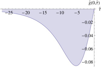
To calculate the perturbations generated by the source (3.23), we must determine the Green’s function for the differential equation (3.42). We can define as the solution to
| (3.47) |
with the boundary conditions across given by
| (3.48) |
It is useful to change variable from to , and solve the simpler equation
| (3.49) |
with the boundary conditions across given by
| (3.50) |
Here a dot stands for a derivative with respect to . Notice that in this way all the dependence on is implicit in the definition of , and we have the simple relation:
| (3.51) |
This change of variables will allow us to see analytically that the power spectrum is scale invariant. The sourced perturbation is given by
| (3.52) |
and the power spectrum at late times () is given by
This shows that the power spectrum is scale invariant. In order to determine its amplitude, we need to perform the integral above in (3.1), where we see that the power spectrum is determined by an ‘effective’ Green’s function
| (3.54) |
with only the term surviving as . Though we have an analytic expression for the ’s 444That we do not reproduce here for the sake of brevity., we are unfortunately unable to perform the integral analytically. However, we can notice that the function , whose only parametric dependence is on , has a peak at the point (corresponding to a physical momentum ), with amplitude and width 555Notice that, as anticipated, in cosmic time, this width corresponds to a time interval of order .. This allows us to estimate the integral (3.1) and to obtain the power spectrum:
| (3.55) |
This expression can be verified numerically.
Finally, we should ensure that our integral approximation was valid in this context. When is large, it is clear that the variation of is large compared to the spacing between particle production events. However, the contribution from the integral only becomes important when the frequency of the modes is . Therefore, the integral is a good approximation when . This condition becomes, using our background solution (2.9),
| (3.56) |
This is a stronger version of the constraints sketched after eq. (2.7).
We derived the integral term assuming that the particle production at each point is the same as for a homogeneous field, which is a valid assumption when the modes of interest obey . Since the integral term becomes important at the freeze-out scale , we must have , which gives
| (3.57) |
This constraint is similar to (and stronger than) eq. (2.5), but the origins of the two constraints are different. In the next section, we will look at how all these constraints fit together in a model with .
Before moving on, let us comment on the role of the fields in the perturbation spectrum. Our model is not a single field model, given that we require many fields in order to slow the inflaton. As such, one might wonder if these extra fields may contribute to the density fluctuations. This is not the case because their mass grows to be large before any modes could freeze out. Specifically, the effective mass of a field is given by . A Hubble time after the field becomes massless, the effective mass is given by . One can check that is equivalent to our constraint (2.5). As a result, the fields are massive compared to the Hubble scale and do not contribute to the curvature perturbation 666It is interesting to consider the fate of these heavy particles. In some regions of our parameter space, they are always lighter than : where and refer to the start and end of inflation. If in other regions they become heavy, they may decay (certainly Planck mass black holes decay rapidly to lighter species of particles)..
However, given the crucial role of the ’s in both the background solution and the generation of perturbations, one must ensure that interactions do not cause them to decay. By construction, the two-body decay is always present. We can ensure that none of our results are affected by this process by requiring that dilution of particles due to expansion is the primary cause of decreasing number density. This is expressed by the constraint . Assuming and we get the condition . Evaluating this expression at the moment the fields are created, leads to the constraint
| (3.58) |
We will impose this constraint on our parameters although it is possible our results would not be significantly affected even in regions where it is violated. The mechanism itself can tolerate some production as long as the energy density from the decaying ’s does not interfere with the perturbations.
Let us also compare our result for the scalar power (3.55) with the curvature perturbation one obtains from the fluctuations in energy density coming from the variance in particle number on the right hand side of Einstein’s equation. We can estimate this contribution as
| (3.59) |
Here is not the curvature perturbation but comes from the components of the metric. The expression (3.59) arises from the Hamiltonian constraint. This contribution is not directly contributing to a measurable power spectrum, but we would like to ensure that the curvature it induces during inflation is negligible.
By going into Fourier space, and using the fact that the fluctuations are evaluated when 777This is due to the fact that the fluctuations average quickly to zero on scales longer than , and therefore the induced metric perturbations become constant after having redshifted up to the scale ., we obtain, after using eq. (3.40):
| (3.60) |
Notice that in this estimate. By comparing with the contribution we have just computed, , we obtain
| (3.61) |
This ratio is the usual slow roll parameter, which is much smaller than in this model. The ratio has to be smaller than because of the constraint coming from non-Gaussianities (see next section). For the specific case we will study in the next section, where , the above expression is also equivalent to eq. (2.21) times an additional suppression from the number of e-foldings, and therefore it is always satisfied in that model.
3.2 Non-Gaussian Perturbations
The size and shape of the non-Gaussian contribution to the perturbations are particularly important for distinguishing between different models of inflation [24]. Since our interactions slow the inflaton on a potential which would otherwise be too steep for inflation, we should expect a substantial non-Gaussian correction to the power spectrum as in [6]. A detailed prediction for the bispectrum requires the calculation of the three-point correlation function of the curvature perturbation, as first completed for single-field slow roll inflation in [25, 26].
Following [23], we can expand the equation of motion (3.1) for the perturbation into first order, second order, and higher order pieces:
| (3.62) |
It is again useful to translate the expanded equation of motion into conformal time, and derive its differential form (as done for the linearized equation in (3.42)). Then we can obtain the second order perturbation by integrating against the Green’s function the terms in the expanded equation of motion which are second order in and . By looking at eq. (3.1), one sees that one contribution comes from the expansion of the term proportional to in the equation of motion, giving a contribution to the second order perturbation of order:
| (3.63) |
Another contribution comes from taking into account the time delay of the perturbation inside the integral, giving rise to a term of the form:
| (3.64) |
Yet another contribution, of order , comes from expanding the coefficient in the source term, giving a contribution
| (3.65) |
There are additional terms coming from the expansion of , but it is easy to see that they give subleading contributions. Also the contribution from the non-Gaussian statistics of which in the absence of interactions can still come from -particle shot noise, is expected to be negligible if the number of particles is large enough. This is in fact always the case. Estimating the size of the non-gaussianity of by , where we have used that is the typical scale at which the Green’s functions peak, it is easy to see that in our model, by using eq. (3.55), this ratio is smaller than , corresponding approximately to a negligibly small .
The three point function of our perturbations is of the form
| (3.66) |
and we are interested in this amplitude at late times, . We can estimate this using the same method we used for the Gaussian power spectrum, and let us start with the term in eq. (3.63). The perturbations on the right hand side of (3.63) can come from any of the three modes (3.44), not only from the constant mode . This is so because the perturbations in that source the second order in eq. (3.63) can be evaluated when still well inside the horizon when neither of the three modes has yet decaied. One of the leading effects we find comes from the and modes 888A similar term with a pair of or a pair of modes will change the final result by no more than an factor. We study the term above because the cancellation between phases is particularly simple., giving a contribution to the three point function of curvature perturbations of order
| (3.67) | |||
| (3.68) |
If we pass to the Green’s functions defined as in the former section, we find:
| (3.69) | |||
where we have defined and . The former expression is of the form
| (3.70) | |||
The factor of , which characterizes the dependence on the global scale of the momenta, tells us that the signal is scale invariant [24].
As we discussed above, the Green’s functions or are peaked at , and the product of integrals forming the integrand also exhibit a peak at this value. We can estimate the size of using knowledge of the peak at and series expansion of the Green’s functions around . We find that the Green’s functions and can be expanded as a series of the form with order one coefficients . Physically, we believe this occurs because the only features of these functions occur near . Therefore, we only expect any non-trivial behavior when . Using the above Taylor expansion at is likely inaccurate, but we think it should be reliable for order of magnitude estimates 999All the results using series expansions have been checked against numerical integrations and provide reliable estimates..
In the language of eq. (3.54), the leading terms in the expansion for are of order and those for are of order . The oscillations contribute a suppression factor to the integrals and an enhancement to the derivatives. Altogether this gives us an estimate, which we checked against a numerical integration, of order
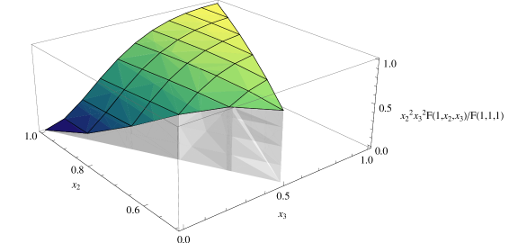
| (3.71) |
Here we were not careful with the momenta dependence, and the factor denotes only the typical size of the wavenumber. A more careful numerical analysis for the shape function as defined in [24] shows that most of the signal is concentrated on equilateral configurations. The equilateral shape can be understood to be a result of the Green’s functions being peaked at a scale : we get a large contribution when all the momenta are equal and all the Green’s functions can be evaluated at their peak value. More in detail, by looking at eq. (3.69), one can notice that in order for the integrals in and to include in their domain the peaks of and of by the time reaches its peak at , we need to have . However, in the limit , we have approximately , which suppresses this contribution to the shape by and forces the dominant contribution to come from the case where are as large as possible compatibly with the former constraint. We obtain that the integrals are peaked for , on equilateral configurations 101010There is some support also on flattened triangles, but the numerical study plotted in Fig. 2 shows that this does not dominate over the equilateral shape.. The suppression of at small comes from the fact that the oscillating modes decay at late time. Notwithstanding the fact that the leading mechanism for generating non-Gaussianities is intrinsically a multifield effect, we conclude that the signal on squeezed configurations is not large, as is always the case in single field inflation [25, 26, 27, 28, 29].
A similar analysis shows that the contribution due to is parametrically the same as the one of , while the one from is suppressed by a factor of . The remaining terms that we did not show are subleading as well. Since we are not careful with order one coefficients, there is no need to perform the calculation for , since we do not expect cancellations or the shape to be peaked in the squeezed limit.
Summarizing, following the standard definition, we can estimate the size on equilateral triangles (with ) to be of order
| (3.72) |
where the primes indicate that we dropped the delta functions of momenta.
4 The case
Let us now check the conditions for a viable model of trapped inflation, including the background solution and Gaussian perturbations. We will take a model with potential for simplicity; other cases of interest include more general power law potentials . Given the number of e-foldings, the Gaussian power spectrum (3.55), and our solution (2.9), we can solve for two of the parameters and then express the various inequalities prescribed in §2 in terms of fewer model parameters. From this, we obtain the following relations.
The number of e-foldings is
| (4.73) |
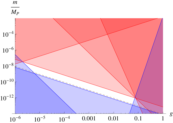
where the slow roll condition (2.15) forced the total field range and we used (3.55) to eliminate . Using this, (3.55), and our solution (2.9) to write the self-consistency conditions in terms of , the constraints (2.16), (2.17), (2.21), (3.56) respectively give four conditions 111111The constraints (2.15), (2.20) give , and so are trivially satisfied.
| (4.74) |
The constraint (3.57) and (3.58) are in the other direction:
| (4.75) |
Together, these constraints define a viable window in the space defined by the two free parameters , which is plotted in Fig. 3. Maximizing the value of the field range over this window, the field range is constrained to lie no more than an order of magnitude above the Planck scale. The mechanism therefore can operate below the scale typically needed for standard slow-roll inflation - in fact the constraints described above allow field values far below although we will see in the next section that experimental constraints on the size of the non-Gaussianity in the power spectrum prevent us from going far below the Planck scale in this model.
5 Observational predictions
In this section we will outline the predictions for the CMB derived from our inflationary mechanism.
5.1 and
Because and other background parameters change slowly during inflation, our power spectrum is approximately scale invariant. Its tilt is given by
| (5.76) |
From (3.55) this becomes
| (5.77) |
where in the next to last passage we used eqs. (4.73) and (3.1), and in the last passage we have used a typical number of e-foldings 121212For potentials of the form , .. The parameter we have introduced here represents the ratio , between the value of at efoldings to the end of inflation and the value at the end of inflation. This parameter was not introduced in the former estimates because it does not affect them significantly. The condition requires that , so we can safely take . The tilt is red, falling quite close to the statistically preferred region of the WMAP 5-year data [30]. However, it is worth mentioning that the tilt may not be a sharp prediction of this class of of models, but may be tunable in general. It can depend not only on the potential and the field range, but also on other details such as variation in the spacing between the particle production events, and in the mass and species numbers of of the particles. In order to compute the tilt very precisely, it would also be important to systematically check the contributions of higher dimension operators. These are limited by symmetries in our string-theoretic backgrounds, but we have not done a complete analysis of their leading effects.
The power in gravity waves is as usual , leading to a tensor to scalar ratio of:
| (5.78) |
in the model. Maximizing this quantity over the allowed range of from the previous section, we find for this potential.
5.2 Non-Gaussianity
Current constraints from data [30, 31] bound so that, using eq. (3.72), we have
| (5.79) |
Note that since we have not been keeping track of factors, there is a possibility that these may shift this constraint slightly in either direction.
Plugging this into our solution, this is equivalent to
| (5.80) |
For this corresponds to
| (5.81) |
and imposing (4.73) we obtain
| (5.82) |
This goes in the opposite direction from the previous conditions (4) (except for (4.75)), but leaves a wide window of viability. As seen in Fig. 3, it is the constraint on the non-Gaussianity that restricts the field range from going far below the Planck scale. This is to be expected - as in [5],[6], as the potential grows steeper a stronger interaction will be needed to slow the inflaton, and a larger contribution to the non-Gaussianity will be produced.
6 Trapped Inflation from String Theory
“Meetings are a great trap…” –John Kenneth Galbraith
Because inflation is sensitive to Planck-suppressed operators in the effective field theory, it is generally of interest to model it in a UV complete theory of gravity. String theory, as a candidate UV completion of gravity, is a standard framework in which to develop such constructions. The present work was motivated in part by the top-down appearance of the structure required for trapped inflation. In this section, we will explain this structure and analyze the conditions for realizing trapped inflation consistently with moduli stabilization in appropriate examples. These realizations use the same structures recently used for monodromy-driven large field inflation [32, 17], but now in a range of field. Because the relevant setups were described in detail in these works, our discussion here will be somewhat more telescopic; the reader may therefore find it easiest to refer back to the relevant portions of [32, 17].
To begin, consider wrapped D4-branes in type IIA string compactifications on nilmanifolds, as in [16, 32]. The simplest example of a Nil manifold suffices to exhibit our basic mechanism for closely spaced particle production events, though we will see that trapped inflation in this specific example would introduce too large a back reaction on the internal geometry. We will therefore ultimately be led to construct it in string theory by using axion moduli in warped Calabi-Yau compactifications of the kind analyzed recently in [17]. Particle production in these models was also considered in [33] where it was used for reheating.
A nil 3-manifold is obtained by compactifying the nil geometry
| (6.83) | |||||
(where ) by a discrete subgroup of the isometry group
| (6.84) |
This manifold can be described as follows. For each , there is a torus in the and directions. Moving along the direction, the complex structure of this torus goes from as . The projection by identifies these equivalent tori 131313The directions and are on the same footing; similar statements apply with the two interchanged and with replaced by ..
At all values for integer , the two-torus in the directions is equivalent to a rectangular torus
| (6.85) |
(since as ). These coordinates and are related to and by an transformation. The 1-cycle traced out by becomes a cycle as .
Consider first, as in [16], a D4-brane wrapped on this cycle. Near , it has a potential energy of the form
| (6.86) |
in terms of the canonically normalized field corresponding to its collective coordinate in the direction. This collective coordinate will play the role of the inflaton, and we will refer to this D4-brane as the inflaton brane.
As mentioned above, at there is a rectangular torus in the directions, equivalent by an SL(2,Z) transformation to the one at the origin. Introduce additional D4-branes wrapped on the corresponding SL(2,Z) transforms of the cycle wrapped by the inflaton brane. The such brane has a quadratic potential proportional to , minimized at . Place each at its minimum. As the inflaton brane rolls down its potential (6.86), it encounters these additional branes, causing the strings (and fermion partners) stretched between them to come down to zero mass. That is, and the couple as in our basic field theory model (1.1).
It is clear that this structure arises more generally than the particular model [32, 16]. In this particular case it is worthwhile to analyze the consistency of these added branes with the moduli stabilization barriers introduced by the curvature of the nilmanifold and other ingredients required to stabilize the space. A single D4-brane at the minimum of its potential is subdominant to the moduli-stabilizing barriers. There is a limit to how many additional branes can coexist with moduli stabilization. The tension of the set of D4-branes is
| (6.87) |
This must be less than the scale of the moduli-stabilizing barriers, of order the curvature-induced potential energy:
| (6.88) |
Now in terms of the field theoretic quantities of the previous sections, . So the condition (6.88) translates into the condition
| (6.89) |
In the simplest version of the construction [32] – with the numerical examples discussed there and in [16] – the number of D4-branes is limited by this back reaction to be of order 10. Possibilities for warping down excessive contributions to the potential energy were discussed in [32]. In general, the mechanism we have discussed arises in a wide variety of “monodrofold” type compactifications [34].
A similar structure, with somewhat more flexibility in the parameters, arises in the setting [17] to construct trapped inflation from string theory. Consider type IIB string theory on a warped Calabi-Yau manifold, with an axion arising from a 2-form RR potential integrated over a 2-cycle . In the presence of an NS5-brane wrapped on within a warped region (with a corresponding anti-brane wrapped on a homologous cycle in a distant warped region), the potential for takes the form
| (6.90) |
where encodes the warp-factor dependence. As explained in [17], the axion decay constant is of order . This setup, with a large stabilized 2-cycle size , naturally realizes large-field inflation (with playing the role of the inflaton, executing many cycles of its basic period ). For the case of a blown-down 2-cycle, , the same setup leads to trapping as follows. When , as rolls through the values (with an integer), new light degrees of freedom appear in the theory. One intuitive way to see this is via the S- and T- dual setup depicted in Fig. 1 of [17] – there the NS5-branes’ horizontal separation corresponds to , and when this vanishes the unwinding motion takes the system through configurations where these NS5-branes meet. At these points, new light degrees of freedom arise from stretched D2-branes; the theory at low energies is a nontrivial interacting CFT (see e.g. [35]). The massless degrees of freedom of this CFT are produced much in the same way as are the ’s described above (though perhaps in this case we should call it unparticle production, since the low-lying degrees of freedom of the CFT are not strictly speaking particle states). In the original duality frame, the light “tensionless string” degrees of freedom arise with from wrapped D3-branes (with appropriate worldvolume flux to cancel the contribution of to the brane tension at the quantized values ).
Of order to circuits can fit inside the compactification, satisfying the back reaction constraint delineated in eqn (3.42) of [17] by using the freedom to obtain somewhat large volume while maintaining high moduli stabilizing barriers using for example the methods of the large volume scenario [36] as explained in §4.4.1 of [17].
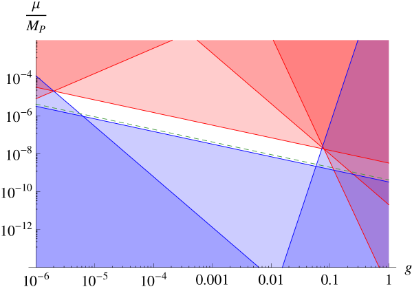
This construction corresponds to a linear potential (modulated by instanton-generated sinusoidal corrections), a simple generalization of the model analyzed above in §4. This potential is slightly flatter but leads to similar conditions on its parameters, shown in figure 3.
Now for a potential , from our solution above we have
| (6.91) |
For , i.e. , this becomes (using (4.73))
| (6.92) |
The number of e-foldings is
| (6.93) |
which reproduces the result (4.73) listed above for the case .
The non-Gaussianity constraint corresponds to (for )
| (6.94) |
For this becomes
| (6.95) |
and for it is
| (6.96) |
This corresponds to a constraint on the number of production events
| (6.97) |
for any . Similarly, one can derive a lower bound on from our slow roll conditions. For a wide range of parameters, the most stringent condition comes from (2.21). For , the constraint is
| (6.98) |
Therefore, for any one has a window of between the minimum and maximum values allowed.
Altogether, we find that the structure required for trapped inflation arises in the directions with monodromy in string compactifications, within a different regime of the potential and field range from that considered in modeling chaotic inflation in [16, 17]. The ingredients required for trapped inflation generally introduce more back reaction than occurs in the corresponding single-field chaotic inflation model, but do fit into a reasonable subset of the known constructions.
7 Discussion
One of the satisfying recent developments in inflationary theory has been a more systematic classification of inflationary mechanisms. An inflationary mechanism can be characterized by its number of degrees of freedom – single field versus multiple field (a feature correlated with and isocurvature effects), the sound speed of its perturbations (correlated with ), and the field range of its inflaton (correlated with the gravity wave signature ). The present mechanism involves multiple fields (including the s), but it behaves like some single field models in its prediction for large .141414See e.g. [37] for an analysis of possible shapes of the non-Gaussianity arising from multifield models with nontrivial kinetic terms.
Although its signatures are somewhat similar to its strong-coupling analogue [6], we have seen that trapped inflation fits concretely into previously studied string compactifications; it is fair to say that the mechanism [5, 6] lacks a known clean top-down embedding (in the small subset of string compactifications yet studied). It would be interesting to find a compactification that interpolates between the two cases by varying the number of light degrees of freedom (and hence the ’t Hooft coupling).
The calculations in this paper required somewhat novel techniques for treating the effective dynamics of resulting from the production of the sets of (temporarily) light particles. There are several ways in which our analysis could be extended. In particular, it would be useful to develop more precise analytical tools to treat the perturbations.
Acknowledgments
We thank Tomas Rube for early collaboration. We thank N. Arkani-Hamed, L. Kofman, A. Linde, X. Liu, L. McAllister, A. Westphal, and M. Zaldarriaga for useful discussions. The research of D.G., B.H., and E.S. is supported by NSF grant PHY-0244728, by the DOE under contract DE-AC03-76SF00515, and by BSF and FQXi grants. D.G. is also supported by a Mellam Family Graduate Fellowship and a NSERC Fellowship. B. H. is also supported by a William K. Bowes Jr. Stanford Graduate Fellowship. The research of LS is supported in part by the National Science Foundation under Grant No. PHY-0503584.
References
- [1] A. H. Guth, “The Inflationary Universe: A Possible Solution To The Horizon And Flatness Problems,” Phys. Rev. D 23, 347 (1981); A. D. Linde, “A New Inflationary Universe Scenario: A Possible Solution Of The Horizon, Flatness, Homogeneity, Isotropy And Primordial Monopole Problems,” Phys. Lett. B 108, 389 (1982); A. Albrecht and P. J. Steinhardt, “Cosmology For Grand Unified Theories With Radiatively Induced Symmetry Breaking,” Phys. Rev. Lett. 48, 1220 (1982).
- [2] C. Cheung, P. Creminelli, A. L. Fitzpatrick, J. Kaplan and L. Senatore, “The Effective Field Theory of Inflation,” JHEP 0803, 014 (2008) [arXiv:0709.0293 [hep-th]].
- [3] C. Armendariz-Picon, T. Damour and V. F. Mukhanov, “k-inflation,” Phys. Lett. B 458, 209 (1999) [arXiv:hep-th/9904075].
- [4] J. Garriga and V. F. Mukhanov, “Perturbations in k-inflation,” Phys. Lett. B 458, 219 (1999) [arXiv:hep-th/9904176]. X. Chen, M. x. Huang, S. Kachru and G. Shiu, “Observational signatures and non-Gaussianities of general single field inflation,” JCAP 0701, 002 (2007) [arXiv:hep-th/0605045].
- [5] E. Silverstein and D. Tong, “Scalar speed limits and cosmology: Acceleration from D-cceleration,” Phys. Rev. D 70, 103505 (2004) [arXiv:hep-th/0310221].
- [6] M. Alishahiha, E. Silverstein and D. Tong, “DBI in the sky,” Phys. Rev. D 70, 123505 (2004) [arXiv:hep-th/0404084].
- [7] X. Chen, “Multi-throat brane inflation,” Phys. Rev. D 71, 063506 (2005) [arXiv:hep-th/0408084].
- [8] L. Kofman and A. Linde, “Pre-Inflation,” pre-preprint, circa 1999. L. Kofman, A. Linde, X. Liu, A. Maloney, L. McAllister and E. Silverstein, “Beauty is attractive: Moduli trapping at enhanced symmetry points,” JHEP 0405, 030 (2004) [arXiv:hep-th/0403001].
- [9] L. Kofman, A. D. Linde and A. A. Starobinsky, “Towards the theory of reheating after inflation,” Phys. Rev. D 56, 3258 (1997) [arXiv:hep-ph/9704452]. J. H. Traschen and R. H. Brandenberger, “Particle Production During Out-of-Equilibrium Phase Transitions,” Phys. Rev. D 42, 2491 (1990). A. D. Dolgov and D. P. Kirilova, “Production of particles by a variable scalar field,” Sov. J. Nucl. Phys. 51, 172 (1990) [Yad. Fiz. 51, 273 (1990)].
- [10] A. Berera, I. G. Moss and R. O. Ramos, “Warm Inflation and its Microphysical Basis,” arXiv:0808.1855 [hep-ph].
- [11] A. Berera and T. W. Kephart, “Ubiquitous inflaton in string-inspired models,” Phys. Rev. Lett. 83 (1999) 1084 [arXiv:hep-ph/9904410].
- [12] N. Kaloper and K. A. Olive, Astropart. Phys. 1, 185 (1993).
- [13] R. Brustein, S. P. de Alwis and P. Martens, “Cosmological stabilization of moduli with steep potentials,” Phys. Rev. D 70, 126012 (2004) [arXiv:hep-th/0408160].
- [14] N. Itzhaki and E. D. Kovetz, “Inflection Point Inflation and Time Dependent Potentials in String Theory,” JHEP 0710, 054 (2007) [arXiv:0708.2798 [hep-th]].
- [15] D. J. H. Chung, E. W. Kolb, A. Riotto and I. I. Tkachev, Phys. Rev. D 62, 043508 (2000) [arXiv:hep-ph/9910437]. A. E. Romano and M. Sasaki, Phys. Rev. D 78, 103522 (2008) [arXiv:0809.5142 [gr-qc]].
- [16] E. Silverstein and A. Westphal, “Monodromy in the CMB: Gravity Waves and String Inflation,” arXiv:0803.3085 [hep-th].
- [17] L. McAllister, E. Silverstein and A. Westphal, “Gravity Waves and Linear Inflation from Axion Monodromy,” arXiv:0808.0706 [hep-th].
- [18] A. D. Linde, “Chaotic Inflation,” Phys. Lett. B 129, 177 (1983).
- [19] N. Arkani-Hamed, P. Creminelli, S. Mukohyama and M. Zaldarriaga, “Ghost inflation,” JCAP 0404, 001 (2004) [arXiv:hep-th/0312100].
- [20] F. R. Bouchet [Planck Collaboration], “The Planck satellite: Status & perspectives,” Mod. Phys. Lett. A 22, 1857 (2007).
- [21] N. Barnaby, Z. Huang, L. Kofman and D. Pogosyan, “Cosmological Fluctuations from Infra-Red Cascading During Inflation,” arXiv:0902.0615 [hep-th].
- [22] J. M. Bardeen, P. J. Steinhardt and M. S. Turner, “Spontaneous creation of almost scale-free density perturbations in an inflationary universe,” Phys. Rev. D 28, 679 (1983).
- [23] I. G. Moss and C. Xiong, “Non-gaussianity in fluctuations from warm inflation,” JCAP 0704, 007 (2007) [arXiv:astro-ph/0701302]. A. Berera, Phys. Rev. D 54, 2519 (1996) [arXiv:hep-th/9601134]. W. Lee and L. Z. Fang, Phys. Rev. D 59, 083503 (1999) [arXiv:astro-ph/9901195]. A. Berera, “Interpolating the stage of exponential expansion in the early universe: A Phys. Rev. D 55, 3346 (1997) [arXiv:hep-ph/9612239]. A. Berera, M. Gleiser and R. O. Ramos, Phys. Rev. D 58, 123508 (1998) [arXiv:hep-ph/9803394]. A. Berera, “Warm inflation at arbitrary adiabaticity: A model, an existence proof for inflationary dynamics in quantum field theory,” Nucl. Phys. B 585, 666 (2000) [arXiv:hep-ph/9904409]. A. N. Taylor and A. Berera, Phys. Rev. D 62, 083517 (2000) [arXiv:astro-ph/0006077]. C. H. Wu, K. W. Ng, W. Lee, D. S. Lee and Y. Y. Charng, JCAP 0702, 006 (2007) [arXiv:astro-ph/0604292]. B. Chen, Y. Wang and W. Xue, JCAP 0805, 014 (2008) [arXiv:0712.2345 [hep-th]].
- [24] D. Babich, P. Creminelli and M. Zaldarriaga, “The shape of non-Gaussianities,” JCAP 0408, 009 (2004) [arXiv:astro-ph/0405356].
- [25] J. M. Maldacena, “Non-Gaussian features of primordial fluctuations in single field inflationary models,” JHEP 0305, 013 (2003) [arXiv:astro-ph/0210603].
- [26] V. Acquaviva, N. Bartolo, S. Matarrese and A. Riotto, “Second-order cosmological perturbations from inflation,” Nucl. Phys. B 667, 119 (2003) [arXiv:astro-ph/0209156].
- [27] P. Creminelli, “On non-gaussianities in single-field inflation,” JCAP 0310, 003 (2003) [arXiv:astro-ph/0306122].
- [28] P. Creminelli and M. Zaldarriaga, “Single field consistency relation for the 3-point function,” JCAP 0410 (2004) 006 [arXiv:astro-ph/0407059].
- [29] C. Cheung, A. L. Fitzpatrick, J. Kaplan and L. Senatore, “On the consistency relation of the 3-point function in single field inflation,” JCAP 0802 (2008) 021 [arXiv:0709.0295 [hep-th]].
- [30] D. N. Spergel et al. [WMAP Collaboration], “First Year Wilkinson Microwave Anisotropy Probe (WMAP) Observations: Determination of Cosmological Parameters,” Astrophys. J. Suppl. 148, 175 (2003) [arXiv:astro-ph/0302209]; H. V. Peiris et al., “First year Wilkinson Microwave Anisotropy Probe (WMAP) observations: Implications for inflation,” Astrophys. J. Suppl. 148, 213 (2003) [arXiv:astro-ph/0302225]; D. N. Spergel et al. [WMAP Collaboration], “Wilkinson Microwave Anisotropy Probe (WMAP) three year results: Implications for cosmology,” Astrophys. J. Suppl. 170, 377 (2007) [arXiv:astro-ph/0603449]. E. Komatsu et al., “Five-Year Wilkinson Microwave Anisotropy Probe (WMAP) Observations: Cosmological Interpretation,” submitted to Astrophys. J. Suppl. [arXiv:0803.0547 [astro-ph]].
- [31] P. Creminelli, L. Senatore, M. Zaldarriaga and M. Tegmark, “Limits on parameters from WMAP 3yr data,” JCAP 0703, 005 (2007) [arXiv:astro-ph/0610600].
- [32] E. Silverstein, “Simple de Sitter Solutions,” Phys. Rev. D 77, 106006 (2008) [arXiv:0712.1196 [hep-th]]; S. S. Haque, G. Shiu, B. Underwood and T. Van Riet, “Minimal simple de Sitter solutions,” arXiv:0810.5328 [hep-th].
- [33] R. H. Brandenberger, A. Knauf and L. C. Lorenz, JHEP 0810, 110 (2008) [arXiv:0808.3936 [hep-th]].
- [34] see e.g. S. Hellerman, J. McGreevy and B. Williams, “Geometric constructions of nongeometric string theories,” JHEP 0401, 024 (2004) [arXiv:hep-th/0208174]. D. Vegh and J. McGreevy, “Semi-Flatland,” arXiv:0808.1569 [hep-th]. A. Lawrence, M. B. Schulz and B. Wecht, “D-branes in nongeometric backgrounds,” JHEP 0607, 038 (2006) [arXiv:hep-th/0602025]. J. Shelton, W. Taylor and B. Wecht, “Generalized flux vacua,” JHEP 0702, 095 (2007) [arXiv:hep-th/0607015].
- [35] N. Seiberg and S. Sethi, “Comments on Neveu-Schwarz five-branes,” Adv. Theor. Math. Phys. 1, 259 (1998) [arXiv:hep-th/9708085].
- [36] V. Balasubramanian, P. Berglund, J. P. Conlon and F. Quevedo, “Systematics of moduli stabilisation in Calabi-Yau flux compactifications,” JHEP 0503, 007 (2005) [arXiv:hep-th/0502058]. J. P. Conlon and F. Quevedo, “On the explicit construction and statistics of Calabi-Yau flux vacua,” JHEP 0410, 039 (2004) [arXiv:hep-th/0409215].
- [37] D. Langlois, S. Renaux-Petel, D. A. Steer and T. Tanaka, “Primordial perturbations and non-Gaussianities in DBI and general multi-field inflation,” Phys. Rev. D 78, 063523 (2008) [arXiv:0806.0336 [hep-th]].