Self-organization, scaling and collapse in a coupled automaton model of foragers and vegetation resources with seed dispersal

Abstract

We introduce a model of traveling agents (e.g. frugivorous animals) who feed on randomly located vegetation patches and disperse their seeds, thus modifying the spatial distribution of resources in the long term. It is assumed that the survival probability of a seed increases with the distance to the parent patch and decreases with the size of the colonized patch. In turn, the foraging agents use a deterministic strategy with memory, that makes them visit the largest possible patches accessible within minimal travelling distances. The combination of these interactions produce complex spatio-temporal patterns. If the patches have a small initial size, the vegetation total mass (biomass) increases with time and reaches a maximum corresponding to a self-organized critical state with power-law distributed patch sizes and Lévy-like movement patterns for the foragers. However, this state collapses as the biomass sharply decreases to reach a noisy stationary regime characterized by corrections to scaling. In systems with low plant competition, the efficiency of the foraging rules leads to the formation of heterogeneous vegetation patterns with $1/f^{\alpha}$ frequency spectra, and contributes, rather counter-intuitively, to lower the biomass levels.

1 Introduction

Animal movement and its ecological implications is a discipline that attracts a growing interest [1]. The study of animal displacements gives valuable clues on how complex organisms adapt to their environment, in particular to search, prepare and consume food [2]. Foraging problems have motivated many modeling approaches, sometimes inspired from the physics of the random walk problem [3]. In a way similar to anomalously diffusing particles in a physical context, the displacement patterns of a variety of animals (albatrosses [4], bumble-bees [4], primates [5], gastropods [6], jackals [7], seals [8] and sharks [9], among others) involve many spatio-temporal scales and are sometimes well described by Lévy walks or intermittent processes with power-law distributions. On a biological point of view, wide fluctuations in the movements of a herbivorous or frugivorous animal are interesting as they may reflect a variety of behavioural responses induced by a complex environment with resources distributed heterogeneously [10, 11, 12, 13].

Plant ecosystems are out-of-equilibrium and exhibit rich structures and dynamics. Spatial patterns in the distribution of plant species are highly non random and contain many characteristic length scales [14]. Patch distributions in rain forests have fractal properties, suggesting that these systems could be near a self-organized critical state driven by the slow growth of trees and sudden mortality avalanches [15]. Other observations report that tree sizes (and therefore fruit contents) in template and tropical forests are distributed according to inverse power-laws [16, 17]. When water resources are a limiting factor, continuous models show that plant interactions produce aggregation in patches that self-organize at larger scales to form more or less regular patterns [18], or disordered ones where patch areas obey scale-free probability distribution functions [19].

Seed dispersal represents an important animal/plant interaction that may contribute to the formation of complex ecological patterns. Seed dispersal at long distances has been identified as an important structuring factor of tree communities [20, 21]. Fruit eating animals (e.g., spider monkeys [22]) swallow the seeds of many tree species and deposit them, through faeces, practically intact and away from the parent tree after a transit time of a few hours. Between 60 and 90$\%$ of the seeds of tree species of tropical forests are dispersed by vertebrates that feed on fruit [23], specially primates [24, 25, 26].

The aim of this article is to study an automaton model of moving foragers that modify, via seed dispersal, the long term structure of the resources they consume. In turn, these resources also determine the foragers displacements, who use cognitive skills to explore their medium in an efficient, non-random way. The model assumes that two factors influence the growth success of a seed: the distance to the parent plant [20] and competition due to the presence of other plants [21]. Despite that the model is over-simplified, the forager/resources coupled dynamics leads to rich behaviours, like self-organized states with power-law statistics for patch sizes and animal movement lengths.

The following two Sections describe the model and its background. The results and the underlying mechanism leading to power-laws in this system are presented in Section 4, and conclusions in Section 5.

2 Background: a foraging model without plant dynamics

We first describe the movement rules of the model forager in a stationary distribution of resource patches (see refs. [13, 27]). Consider a two-dimensional square domain of area unity containing $N$ fixed, point-like patches randomly and uniformly distributed. To each patch $i$ is assigned a fixed size (or food content), $k_{i}=1,2...$, a integer drawn from a given distribution, $p(k)$.

Like many other animals, primates use cognitive maps to navigate their environment [28, 29]. Evidence shows that travels to fruiting trees are more frequent than as suggested by random null models [29]. Primates also keep record of the sites they have visited in a recent past [28]. For simplicity, we assume that our model forager has a perfect knowledge of the positions and sizes of all the patches in the system. Initially, a forager is located on a patch chosen at random. The following deterministic foraging rules are then iteratively applied at every time step ($t\rightarrow t+1$):

(i) The forager located at patch $i$ feeds on that patch, the fruit content decreasing by one unit: $k_{i}\rightarrow k_{i}-1$.

(ii) If $k_{i}$ has reached the value 0, the forager chooses an other patch, $j$, such that $k_{j}/d_{ij}$ is maximal over all the allowed patches $j\neq i$ in the system, where $k_{j}$ is the food content of patch $j$ and $d_{ij}$ the Euclidean distance between patches $i$ and $j$. With this rule, the next visited patch (the “best” patch) has a large food content and/or is at a short distance from $i$. We assume that the travel from $i$ to $j$ takes one time unit.

(iii) The forager does not revisit previously visited patches.

This model produces complex trajectories that have been studied in details in refs. [13, 27] and discussed in connection with spider monkeys foraging patterns observed in the field [5].

The model has a remarkable property, of interest in the following. Let us define the forager mean-displacement $R(t)$ as $\langle|{\bf r}(t+t_{0})-{\bf r}(t_{0})|\rangle$ with ${\bf r}(t)$ the forager position at time $t$, the averages being taken over different times $t_{0}$ and independent disorder realizations. At fixed patch number $N$ and time $t$, if the resource size distribution is the inverse power-law $p(k)=ck^{-\beta}$ with $\beta=3$, then the mean displacement $R(t)$ is maximal [13]. In other words, media with this size distribution induce maximal displacements, see figure 1. (This property still holds if the forager travels at constant velocity instead of moving in one time unit from one patch to the other [13].)

The feature above can be understood qualitatively by noting that if the medium is very homogeneous (say, $\beta\gg 1$), then all patches are similar in size: given rule (ii), the forager chooses essentially nearby patches. Trajectories are thus composed of small steps and diffusion is relatively slow [13]. On the contrary, if the medium is very heterogeneous ($\beta\simeq 1$), patches with $k_{i}\gg 1$ are numerous: the forager often performs a large step to reach a very good patch and stays there a long time feeding, given rule ${\it(i)}$. The forager activity is dominated by these long trapping times, resulting in very slow (nearly frozen) diffusion. An intermediate situation corresponds to $\beta=3$, for which the best patch from a given point is often far away (at distances much larger than the typical distance between nearest-neighbour patches), but these good patches still have reasonable sizes, so that the forager does not remain trapped feeding on them during very long periods of time.

Figure 1: Numerically obtained mean displacement (in unit of $l_{0}=N^{-1/2}$) as a function of time for the model forager in a random medium with resources size distributed as $p(k)=Ck^{-\beta}$ ($N=10^{6}$).

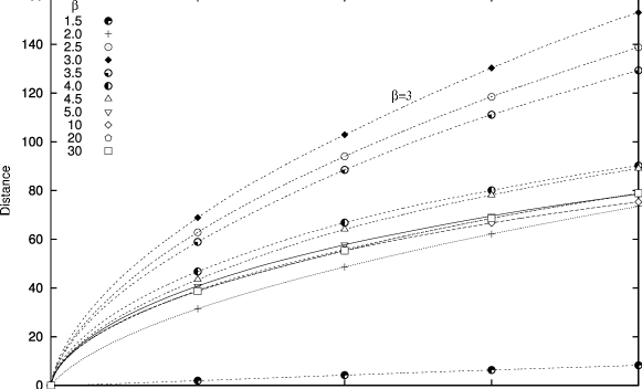
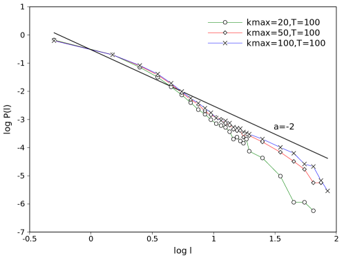
Let us note that, at the special resource exponent value $\beta=3$, the trajectory of the forager closely resembles a Lévy flight. Numerical simulations show that the distribution function of the distances separating successively visited patches is asymptotically given by the power-law [13, 27]

$$P(l)\sim l^{-2}.$$ (1)

The foraging patterns of spider monkeys are well described by the distribution (1) [5, 13]. Even more, these animals feed on trees whose size distribution obeys $p(k)\sim k^{-\beta}$ with $\beta\simeq 2.6$, a value close to 3 [13].

3 Modified model with plant dynamics

In the previous model, forager motion is induced by the medium. In the generalization considered from now on, the forager follows the same rules but also modifies its environment through seed dispersal. Hence, the distribution of resource sizes, $p(k)$, is no longer held fixed and can slowly change over time. We assume that foragers are the main mechanism of seed dispersal.

At $t=0$, $N$ point-like patches, all with size $k_{i}=1$, are randomly and uniformly distributed in the square domain of unit area. A forager initially located on a patch chosen at random follows the rules (i)-(iii) above. In addition,

(iv) every $\tau_{d}$ time units (the digestion time), a seed is deposited at the patch where the forager is located;

(v) every $\tau_{walk}(\gg\tau_{d})$ time units, the walk ends and the forager is removed; the patches are refreshed to their initial $k_{i}$ values; the patches that have received a seed that has survived (see below) increase their size by one unit, $k_{i}\rightarrow k_{i}+1$;

(vi) a new forager (i.e. not representing necessarily the same individual, but still having a perfect knowledge of the updated environment) is located on a patch chosen at random and the process is iterated as above for another $\tau_{walk}$ time units;

(vii) a plant that has grown from a seed deposited $\tau_{m}$ time units earlier ($\tau_{m}\gg\tau_{walk}$) dies and the patch size decreases, $k_{i}\rightarrow k_{i}-1$;

(viii) in rule (vii), the size of a patch does not decrease below the minimal value $k_{i}=1$.

We assume that two factors determine the survival probability of a deposited seed (or the growth success of a plant here) in stage (v). The first assumption is based on observations that seeds dispersed far away survive better, as they are less likely to attract seed predators and to be transmitted parasites or diseases from the parent plant [20]. The second assumption takes into account competition among plants for limited nutrients [21]. Let us note $k$ the size of the patch where the seed is deposited and $l$ its distance to the parent patch, which is the patch where the forager was located $\tau_{d}$ time units ago. The survival probability of the seed, $P_{s}$, is set to $P_{s}=P_{d}(l)P_{c}(k)$ with

$$P_{d}(l) = \left[l/(l+l_{0})\right]^{n},$$ (2)

$$P_{c}(k) = \left\{\begin{array}[]{ll}1-\frac{k}{k_{max}+1}&{\rm if}\ k\leq k_{max}\\ 0&{\rm if}\ k>k_{max},\end{array}\right.$$ (5)

with $l_{0}=N^{-1/2}$ the typical distance between nearest-neighbour patches and $k_{max}$ a fixed integer accounting for competition effects. The parameter $k_{max}$ is proportional, say, to the nutrients concentration. According to (2), the survival probability increases from 0 to 1 as the distance from the parent patch increases, whereas it decreases from 1 to 0 as the size of the colonized patch increases from 1 to $k_{max}$, the maximum patch size. In the following, we fix $n=1$ in Eq.(2), the results presented below being not qualitatively modified if larger values of $n$ are chosen.

4 Results

It is natural to ask the following question. Given that in the model the survival probability increases with the distance to the parent plant and that the largest forager displacements are produced in media with the size distribution $p(k)\sim k^{-3}$, do resources self-organize towards this particular scaling-law (and foraging patterns towards the Lévy law (1))? As a consequence of the memory-based foraging rules (i)-(iii), such environments should have the highest average biomass production rate. As the foragers start dispersing seeds, small heterogeneities are produced ($k_{i}\neq 1$), and, from a dynamical system point of view, the fastest growing modes may dominate the dynamics asymptotically.

Figure 2: Time series (in units of $\tau_{walk}$) of the biomass, for two values of the competition parameter $k_{max}$. The parameters are $N=10^{4}$, $\tau_{d}=10$, $\tau_{walk}=500$ and $\tau_{m}=5\ 10^{4}$.

Successful seeds contribute to the emergence of larger, more attractive patches that are also susceptible of being visited more often in the future. This positive feedback loop contributes to the increase of heterogeneities, within some limits. If very big patches are produced, due to rule (i) many seeds will be dispersed at the distance $l=0$ and will die, given the kernel (2). The other stabilizing effects are competition and mortality.

4.1 The rise and fall of scaling

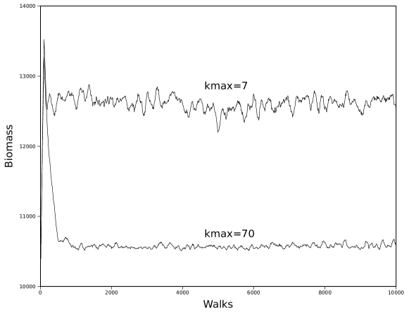
To investigate the possibility of the scenario sketched above, let us first consider the behaviour of the system biomass, $M=\sum_{i=1}^{N}k_{i}$, as a function of time. As displayed in figure 2, $M$ initially increases and reaches a maximum value. It then suffers a abrupt drop, followed by a noisy stationary regime. The asymptotic average biomass depends strongly on plant competition: unexpectedly, it is lower at low competition levels (large $k_{max}$).

The system actually builds spatial heterogeneities during the initial growth regime. Biomass is maximum at $t_{max}=\tau_{m}=(100\tau_{walk}$, here), when the first plants grown from dispersed seeds start to die. As shown by figure 3, the size distribution $p(k)$ at $t=\tau_{m}$ is perfectly fitted by the power-law $k^{-3}$ for $k\ll k_{max}$, independently of the value of $k_{max}$. At the same time, and as expected from Eq.(1), the forager step length distribution (figure 4) tends to the scaling-law $P(l)\sim l^{-2}$ in a range of intermediate values of $l$, with a truncation at large $l$ due to finite $k_{max}$, $\tau_{m}$ and $N$. Note the existence of steps of order of the system size ($100l_{0}$, here). In some sense, the system self-organizes into a critical state of maximal dispersion.

Figure 3: Patch size distributions (in log-decimal representation) for $k_{max}=20$ (left) and $k_{max}=50$ (right), at two different times: $t_{max}(=100\tau_{walk},$ here), when the biomass is maximum (see fig.2), and $t=5000\tau_{walk}$, in the stationary regime. Averages are performed over $10^{3}$ independent initial conditions. The straight lines have a slope $-3$.

Figure 4: Forager step length distributions at $t_{max}$, when biomass is maximal, for $k_{max}=20,50$ and $100$. The straight line has a slope $-2$.

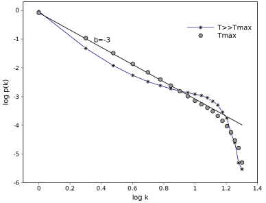
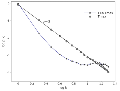
Interestingly, this scaling behaviour does not persist at larger times $t\gg\tau_{m}$. Simultaneously to the biomass collapse (Fig.2), corrections to scaling appear. Asymptotically, the shape of the patch distribution decreases rapidly with patch size and exhibits a practically constant fat tail, see figure 3. Hence, most patches have a small characteristic size and coexist with a few “outliers” of size of order $k_{max}$. This separation into two characteristic sizes becomes more pronounced at large $k_{max}$.

Unexpectedly, dispersal by animals does not manage to stabilize the critical state for which it is responsible. Despite that the system rapidly self-organizes into a state with optimal seed survival, it becomes overpopulated: mortality is much higher than birth shortly after $\tau_{m}$ and the size of many intermediate patches start to shrink. This feature is probably due to the fact that, at $t=\tau_{m}$, the system is much more crowded with plants than at $t=0$. The birth rate is therefore lower than in the initial growth regime because of higher competition (Eq.(5)): older dying plants are not replaced by the same quantity of new ones. In addition, due to their cognitive maps and the rules (i)-(iii), foragers neglect many small, unattractive patches, among them the shrinking ones, that would be suitable for plant growth. Instead, they keep revisiting a small number of nearly saturated large patches (outliers).

4.2 Biomass in the stationary regime

Figure 5: Left: Mean value of the biomass in the stationary regime for several values of the parameter $k_{max}$. Averages are performed over 100 independent runs. The curve has a maximum at $k_{max}=7$ (corresponding to a fairly strong plant competition) and a bistable region centered around $k_{max}=58$ (low plant competition). Same parameters as in Fig. 2. Right: Log-decimal power spectrum $S(f)\equiv\langle\tilde{M}(f)\tilde{M}(-f)\rangle$, with $\tilde{M}(f)$ the Fourier transform of the biomass $M(t)$ in the stationary regime (see figure 2), for $k_{max}=2,7,20$ and $60$. Averages are taken over 60 runs. The straight line is a power-law with exponent $-1.4$.

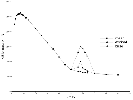
Asymptotically, foragers therefore concentrate their activity on a fraction of the available land, resulting in a reduced biomass. Figure 5 (left) displays the average biomass in the stationary regime as a function of the maximum allowed patch size, $k_{max}$ (or nutrients concentration). Counter-intuitively, but in agreement with the comments above, the general tendency is a biomass decrease with increasing $k_{max}$. The biomass is large at small $k_{max}$ (relatively low nutrients/high competition regime) and presents an extrema at $k_{max}=7$. At this parameter value, patches are relatively homogeneous in size: via foragers visits, seeds can colonize many different patches. At higher $k_{max}$, foragers start to visit large patches preferentially, neglecting smaller ones.

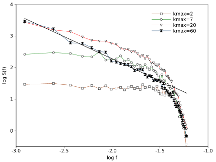
Supporting this interpretation, the power-spectra of the biomass time series $M(t)$ reveal an increase in complexity with increasing $k_{max}$, see figure 5 (right). At high competition levels ($k_{max}=2$), the fluctuations of $M(t)$ around its mean value are due to births and deaths that occur in a roughly independent way, due to a homogeneous dispersion of seeds. The spectrum is that of a white noise. At low competition ($k_{max}=60$), the power spectrum is well approximated by a power-law $1/f^{\alpha}$ with $\alpha\simeq 1.4$ over more than one decade, indicating long-range temporal correlations. The spatially heterogeneous colonization of plants generates periods of high mortality (“avalanches”) of widely varying durations, followed by periods of easier recolonization. This dynamics is obviously reminiscent of the punctuated relaxation of sand-pile models in self-organized criticality [30].

An other unexpected phenomena is observed at low competition levels, in the interval $50<k_{max}<70$ for the parameter values considered here. In this interval, the average biomass increases again and exhibits a second maximum at $k_{max}\simeq 58$. A closer look reveals that the system actually converges towards two distinct states, depending on the initial condition. At identical parameters values, the system sometimes ends up in a low, “base” biomass level that follows the tendency described above, and sometimes exhibits a significantly higher biomass (“excited” state). Biomass fluctuations are relatively small among different systems belonging to a same class (base or excited), which makes possible the computation of the mean values separately (see figure 5). The origin of this bistability is unclear, although it is a known phenomenon in other models of vegetation pattern formation [18].

5 Discussion and conclusions

We have proposed a new mechanism leading to the emergence of many spatio-temporal scales in the movement patterns of foraging animals. In the model proposed, foragers use mental maps to choose feeding patches and disperse seeds along their trajectories, thus affecting the long term distribution of their food resources. This simplified model focuses on plant-forager interactions, neglecting other important factors (wind, gravity…) of seed dispersal [21]. It is built on a generalization of a previous model, where scale-free displacement patterns of knowledgeable animals emerge from their interaction with resources that are distributed according to an a priori given power-law function [13, 27]. In the field, the distributions of the movements of spider monkeys and of the size of their fruiting trees are in good agreement with those given by that model for a particular parameter value, where animal displacements are maxima [13].

The present approach shows that a memory-based ranging behaviour generates highly heterogeneous seed deposition patterns, a conclusion also reached in ref. [26] with the use of a spatially explicit model parameterized with field-collected spider monkeys movement data. These findings suggest that, over large temporal scales, tree distributions may form complex spatial structures due to the presence of foraging animals. The present model proposes a theoretical test of this hypothesis: the distribution of resources is not held fixed and spatial heterogeneities self-organize spontaneously under the influence of positive feedback loops in the system dynamics.

Other existing theories of Lévy [4] or intermittent [31, 32] foraging assume that animals are memoryless and do not have any information on the location of resource patches. In these contexts, they execute a given Markovian stochastic processes to find preys (usually randomly distributed in space) that are detectable only at short distance. Movements with nontrivial distributions or rules are optimal for finding preys most efficiently in some cases. Whereas this approach can be justified for marine animals foraging in unpredictable environments [9], frugivorous vertebrates rely on fixed resources and memory plays an essential role [28, 29]. Nevertheless, the introduction of limited knowledge and the use of search modes would improve the realism of the modelling approach presented here.

Despite that, at each step, our model foragers maximize an efficiency function, their foraging activity can not be considered as optimal in the long term. The hypothesized relationship between long distance dispersal and species diversity in plant communities [13] is probably not a simple one [33]. The model exhibits sudden plant mortality avalanches that are consequences of a restricted land use and a lack of colonization of regions with low plant density. Counter-intuitively, biomass levels are lower when the conditions for colonization are favourable, i.e. at low plant competition levels. The same mechanism leading to the emergence of the self-organized critical state with optimal seed dispersal is also responsible for its rapid collapse. This ecological “crash” is the product of an intelligent foraging behaviour based on the satisfaction of immediate needs (feeding). Here, foragers do not change their strategy when plant resources start to shrink. It would be interesting to investigate whether the introduction of noise (or “irrationality”) in the deterministic decision rules improves this situation.

The model developed here is similar in some aspects to sand-pile models of self-organized criticality (SOC) [30]. The system is driven by successful dispersed seeds and biomass dissipated by mortality. SOC-like models have been proposed to explain large extinctions in the fossil record [34] and tree dynamics on ecological time-scales in rain forests [15]. In the latter example, $1/f$-noise signals have been identified in simulated biomass time series [15] (unfortunately, biomass in real forests is very difficult to measure). Qualitatively similar results are obtained here with other assumptions. The stationary regime of our model, however, is not strictly speaking asymptotically critical since the shape of the patch size distribution contains two characteristic sizes: a small one, of order 1, and a much larger one, corresponding to the presence of “outliers”. Such distributions seem to be ubiquitous in driven self-organized systems, though: they appear in earthquake models [35] and also in other models of plant dynamics in the presence of limited nutrients [19].

The robustness of the features described above should be tested by modifying the foraging rules and the dispersion kernels. A more realistic, resource-dependent forager demography is an aspect that should also be considered.

References

- [1] Nathan R, Getz W M, Revilla E, Holyoak M, Kadmon R, Saltz D and Smouse P E 2008 Proc. Natl. Acad. Sci. USA 105 19052–59
- [2] Stephens D W and Krebs J R 1986 Foraging Theory (Princeton: Princeton University Press)
- [3] Turchin P 1998 Quantitative analysis of movement: Measuring and modelling population redistribution in animals and plants (Sunderland, Massachusetts: Sinauer Associates)
- [4] Viswanathan G M, Buldyrev S V, Havlin S, da Luz M G E, Raposo E P and Stanley H E 1999 Nature 401 911–14
- [5] Ramos-Fernández G, Mateos J L, Miramontes O, Cocho G, Larralde H and Ayala-Orozco B 2004 Behav. Ecol. Sociobiol. 55 223–30
- [6] Seuront L, Duponchel A C and Chapperon C 2007 Physica A 385 573–82
- [7] Atkinson R P D, Rhodes C J, MacDonald D W and Anderson R M 2002 Oikos 98 134–40
- [8] Austin D, Bowen W D and McMillan J I 2004 Oikos 105 15–30
- [9] Sims D W, Southall E J, Humphries N E, Hays G C, Bradshaw C J A, Pitchford J W, James A, Ahmed M Z, Brierley A S, Hindell M A, Morritt D, Musyl M K, Righton D, Shepard E L C, Wearmouth V J, Wilson R P, Witt M J and Metcalfe J D 2008 Nature 451 1098–102
- [10] Hassell M P and May R M 1974 J. Anim. Ecol. 43 567–94
- [11] Benhamou S and Bovet P 1989 Anim. Behav. 38 375–383
- [12] Benhamou S 2007 Ecology 88 1962–69
- [13] Boyer D, Ramos-Fernández G, Miramontes O, Mateos J L, Cocho G, Larralde H, Ramos H and Rojas F 2006 Proc. R. Soc. B 273 1743–50
- [14] Condit R, Ashton P S, Baker P, Bunyavejchewin S, Gunatilleke S, Gunatilleke N, Hubbell S P, Foster R B, Itoh A, LaFrankie J V, Seng Lee H, Losos E, Manokaran N, Sukumar R and Yamakura T 2000 Science 288 1414–18
- [15] Solé R V and Manrubia S C 1995 J. Theor. Biol. 173 31–40
- [16] Enquist B J and Niklas K J 2001 Nature 410 655–60
- [17] Niklas K J, Midgley J J and Rand R H 2003 Ecol. Lett. 6 405–11
- [18] von Hardenberg J, Meron E, Shachak M and Zarmi Y 2001 Phys. Rev. Lett. 87 198101
- [19] Manor A and Shnerb N M 2008 J. Theor. Biol. 253 838–42
- [20] Janzen D H 1970 Am. Nat. 104 501–28
- [21] Nathan R and Muller-Landau H C 2000 Trends Ecol. Evol. 15 278–85
- [22] Lambert J E 1998 Evol. Anthropol. 9 8–20
- [23] Jordano P 1992 Fruits and frugivory The Ecology of Regeneration in Plant Communities ed M Fenner (New York: CAB International) pp 105–56
- [24] Clark C J and Poulsen J R 2001 Biotropica 33 606–20
- [25] Wehncke E, Hubbell P, Foster R B and Dalling W 2003 J. Ecol. 91 677–85
- [26] Russo S E, Portnoy S and Augspurger C K 2006 Ecology 87 3160–74
- [27] D Boyer, O Miramontes and H Larralde 2009 J. Phys. A: Math. Theor. this issue
- [28] Garber P A 1989 Am. J. Primatol. 19 203–16
- [29] Janson C H 1998 Anim. Behav. 55 1229–43
- [30] Bak P, Tang C and Wiesenfeld K 1987 Phys. Rev. Lett. 59 381–84
- [31] Bénichou O, Coppey M, Moreau M, Suet P H and Voituriez R 2005 Phys. Rev. Lett. 94 198101
- [32] Oshanin G, Wio H S, Lindenberg K and Burlatsky S F 2007 J. Phys.: Condens. Matter 19 065142
- [33] France K E and Duffy J E 2006 Nature 441 1139–43
- [34] Bak P and Sneppen K 1993 Phys. Rev. Lett. 71 4083–86
- [35] Gil L and Sornette D 1996 Phys. Rev. Lett. 76 3991–94