Signatures for flow effects in $\sqrt{s}=200$ GeV proton-proton collisions.

Abstract

A simple model based on relativistic geometry and final-state hadronic rescattering is used to predict pion source parameters extracted in two-pion femtoscopy studies of proton-proton collisions at $\sqrt{s}=200$ GeV. From studying the momentum and particle multiplicity dependences of these parameters in the context of this model and assuming a very short hadronization time, flow-like behavior is seen which resembles the flow behavior commonly observed in relativistic heavy-ion collisions.

In the field of fluid dynamics, where a fluid can be either a liquid or a gas, fluid flow is generally defined as the transport of a certain amount of fluid mass or volume across a surface in a given time interval. This concept of fluid flow has been adopted by the relativistic heavy-ion collision community to describe the behaviors of some observables seen in experiments which appear to be flow-like in nature rhic1 ; rhic2 ; rhic3 ; rhic4 . The justification for having a fluid dynamics picture of a relativistic heavy-ion collision is that in these collisions, for example colliding beams of $Au+Au$ at 200 GeV per nucleon pair in the center-of-mass frame, thousands of particles such as partons, e.g. quarks and gluons, hadrons, e.g. nucleons and pions, and leptons, e.g. electrons and muons, participate and are generated out of the vacuum in a violent collision. Thus the concept of characterizing the “bulk properties” of such collisions, for example the dynamics of the size and shape of the interaction region, by a relativistic fluid flow where the fluid is made up of thousands of particles seems reasonable to some approximation. On the other hand, if one were to try to impose a fluid dynamics picture on proton-proton collisions at similar energies, e.g. $p+p$ collisions at $\sqrt{s}=200$ GeV, in which typically much fewer than 100 particles participate and are produced in the collision, such an approximation would seem unreasonable due to the paucity of particles available to compose the “fluid.”

The goal of the present work is to use a simple model to study one of these bulk properties in $p+p$ collisions at $\sqrt{s}=200$ GeV, namely the dynamics of the size and shape of the interaction region, using the method of two-pion femtoscopy Humanic:2006a ; Lisa:2005a also known as Hanbury-Brown-Twiss interferometry (or HBT, which has also been used to measure the sizes of starsHumanic:2006a ; hbt1 ). The HBT observables, which are radius parameters, have been shown in $Au+Au$ collisions at $\sqrt{s_{NN}}=200$ GeV to exhibit radial flow-like behavior in their dependences on the pion momenta and the particle multiplicity of the collision, such that the radius parameters decrease for increasing pion momenta (higher velocity fluid with smaller correlation length) and increase for increasing particle multiplicity (higher density fluid producing more expansion)Adams:2004yc . If the model predicts that there are similar dependences also present in $p+p$ collisions at $\sqrt{s}=200$ GeV it would help to establish the possibility of flow-like effects in these collisions as well as characterize the mechanism by which these effects are generated.

The model calculations are carried out in four main steps: 1) simulate $p+p$ collisions using the standard collision-generator code PYTHIApythia6.4 , 2) employ a simple space-time geometry picture for the hadronization of the PYTHIA-generated hadrons, 3) calculate the effects of final-state rescattering among the hadrons, and 4) calculate the HBT radius parameters. These steps will now be discussed in more detail.

The $p+p$ collisions were modeled with the PYTHIA code, version 6.409 pythia6.4 . The parton distribution functions used were the same as used in Ref. Humanic:2006ib . Events were generated in “minimum bias” mode, i.e. setting the low-$p_{T}$ cutoff for parton-parton collisions to zero and excluding elastic and diffractive collisions. To obtain good statistics for this study $5\times 10^{6}$ events were generated with $\sqrt{s}=$ 200 GeV. Information saved from a PYTHIA run for use in the next step of the procedure were the momenta and identities of the “direct” (i.e. redundancies removed) hadrons (all charge states) $\pi$, $K$, $p$, $n$, $\Lambda$, $\rho$, $\omega$, $\eta$, ${\eta}^{\prime}$, $\phi$, and $K^{*}$. These particles were chosen since they are the most common hadrons produced and thus should have the greatest effect on the hadronic observables in these calculations.

The space-time geometry picture for hadronization from a $p+p$ collision in the model consists of the emission of a PYTHIA particle from a thin uniform disk of radius 1 fm in the $x-y$ plane followed by its hadronization which occurs in the proper time of the particle, $\tau$. The space-time coordinates at hadronization in the lab frame $(x_{h},y_{h},z_{h},t_{h})$ for a particle with momentum coordinates $(p_{x},p_{y},p_{z})$, energy $E$, rest mass $m_{0}$, and transverse disk coordinates $(x_{0},y_{0})$, which are chosen randomly on the disk, can then be written as

$$x_{h}=x_{0}+\tau\frac{p_{x}}{m_{0}}$$ (1)

$$y_{h}=y_{0}+\tau\frac{p_{y}}{m_{0}}$$ (2)

$$z_{h}=\tau\frac{p_{z}}{m_{0}}$$ (3)

$$t_{h}=\tau\frac{E}{m_{0}}$$ (4)

The simplicity of this geometric picture is now clear: it is just an expression of causality with the assumption that all particles hadronize with the same proper time, $\tau$. A similar hadronization picture has been applied to $e^{+}-e^{-}$ collisionscsorgo and Tevatron $p+p$ collisionsHumanic:2006ib . For all results presented in this work, $\tau$ will be set to 0.1 fm/c to be consistent with the results found in the Tevatron study which had reasonable agreement with measurements.

The hadronic rescattering calculational method used is similar to that employed in previous studies Humanic:2006a ; Humanic:2006ib . Rescattering is simulated with a semi-classical Monte Carlo calculation which assumes strong binary collisions between hadrons. Relativistic kinematics is used throughout. The hadrons considered in the calculation are the most common ones: pions, kaons, nucleons and lambdas ($\pi$, K, N, and $\Lambda$), and the $\rho$, $\omega$, $\eta$, ${\eta}^{\prime}$, $\phi$, $\Delta$, and $K^{*}$ resonances. Although $\Delta$ formation was included in the rescattering process due to its large formation cross section in meson-baryon and baryon-baryon rescattering, they were not input directly from PYTHIA since they decay quickly and relatively few are initially produced in these collisions. For simplicity, the calculation is isospin averaged (e.g. no distinction is made among a $\pi^{+}$, $\pi^{0}$, and $\pi^{-}$). Starting from the initial stage ($t=0$ fm/c), the positions of all particles in each event are allowed to evolve in time in small time steps ($\Delta t=0.1$ fm/c) according to their initial momenta. At each time step each particle is checked to see a) if it has hadronized ($t>t_{h}$, where $t_{h}$ is given in Eq. (4)), b) if it decays, and c) if it is sufficiently close to another particle to scatter with it. Isospin-averaged s-wave and p-wave cross sections for meson scattering are obtained from Prakash et al.Prakash:1993a and other cross sections are estimated from fits to hadron scattering data in the Review of Particle Physicspdg . Both elastic and inelastic collisions are included. The calculation is carried out to 50 fm/c which allows ample time for the rescattering to finish. Note that when this cutoff time is reached, all un-decayed resonances are allowed to decay with their natural lifetimes and their projected decay positions and times are recorded. The validity of the numerical methods used in the rescattering code have recently been studied using the subdivision method, the results of which have verified that the methods used are valid Humanic:2006b .

In carrying out a two-pion HBT study the two-pion coincident count rate is calculated along with the one-pion count rates for reference. The two-pion correlation function for pions binned in momenta $\mathbf{p_{1}}$ and $\mathbf{p_{2}}$, $C(\mathbf{p_{1}},\mathbf{p_{2}})$, is constructed event-by-event from the coincident countrate, $N_{2}(\mathbf{p_{1}},\mathbf{p_{2}})$ and one-pion countrate summed over events, $N_{1}(\mathbf{p})$, as

$$C(\mathbf{p_{1}},\mathbf{p_{2}})=\frac{N_{2}(\mathbf{p_{1}},\mathbf{p_{2}})}{N_{1}(\mathbf{p_{1}})N_{1}(\mathbf{p_{2}})}.$$ (5)

It is usually convenient to express the six-dimensional $C(\mathbf{p_{1}},\mathbf{p_{2}})$ in terms of the four-vector momentum difference, $Q=|p_{1}-p_{2}|$ by summing Eq.(5) over momentum difference,

$$C(Q)=\sum_{\mathbf{p_{1}},\mathbf{p_{2}}(Q)}\frac{N_{2}(\mathbf{p_{1}},\mathbf{p_{2}})}{N_{1}(\mathbf{p_{1}})N_{1}(\mathbf{p_{2}})}=\frac{A(Q)}{B(Q)},$$ (6)

where $A(Q)$ represents the “real” coincident two-pion countrate and $B(Q)$ the “background” two-pion countrate composed of products of the one-pion countrates, all expressed in $Q$. Lisa:2005a In practice, $B(Q)$ is the mixed event distribution, which is computed by forming pion-pairs from different events.

For the HBT calculations from the model, a three-dimesional two-pion correlation function is formed using Eq.(6) and a Gaussian function in momentum difference variables is fitted to it to extract the pion source parameters similar to what is done in experimentsHumanic:2006a ; Lisa:2005a . Boson statistics are introduced after the rescattering has finished using the standard method of pair-wise symmetrization of bosons in a plane-wave approximation Humanic:1986a . The three-dimensional correlation function, $C(Q_{side},Q_{out},Q_{long})$, is then calculated in terms of the momentum-difference variables $Q_{side}$, which points in the direction of the sum of the two pion momenta in the transverse plane, $Q_{out}$, which points perpendicular to $Q_{side}$ in the transverse plane and the longitudinal variable along the beam direction $Q_{long}$.

The final step in the calculation is extracting fit parameters by fitting a Gaussian parameterization to the model-generated two-pion correlation function given by, Lisa:2005a

$$C(Q_{side},Q_{out},Q_{long})=$$

$$G[1+\lambda\exp(-Q_{side}^{2}R_{side}^{2}-Q_{out}^{2}R_{out}^{2}-Q_{long}^{2}R_{long}^{2}]$$

where the $R$-parameters, called the radius parameters, are associated with each momentum-difference variable direction, G is a normalization constant, and $\lambda$ is the usual empirical parameter added to help in the fitting of Eq. (Signatures for flow effects in $\sqrt{s}=200$ GeV proton-proton collisions.) to the actual correlation function ($\lambda=1$ in the ideal case). The fit is carried out in the conventional LCMS frame (longitudinally comoving system) in which the longitudinal pion pair momentum vanishes Lisa:2005a .

Figure 1 shows a sample three-dimensional correlation function from the model projected onto the $Q_{side}$ axis with projected fit to Eq. (Signatures for flow effects in $\sqrt{s}=200$ GeV proton-proton collisions.). The other variables, $Q_{out}$ and $Q_{long}$, are integrated up to 0.02 GeV/c. The cuts on the pion momenta are $-0.5<y<0.5$, where y is rapidity, $0.15<p_{T}<0.8$ GeV/c, where $p_{T}$ is transverse momentum, and $0.15<k_{T}<0.25$ GeV/c (see below). These cuts in $y$ and $p_{T}$ are used throughout to duplicate those used in experiments. Although only a small fraction of the full correlation function is shown in this plot, it gives some idea of the quality of the Gaussian fit to the model. For $Q_{side}<0.05$ GeV/c the fit is seen to undershoot the model which is a common feature also seen in experiments for $p+p$ collisionsAlexopoulos:1992iv ; Bailly:1988zb . The $\lambda$ parameter for this fit is 0.330, which is far less than the ideal value of unity, another feature commonly seen in $p+p$ experiments. The source of this non-Gaussian and non-ideal behavior in the model is the presence of medium to long-lived resonances such as the $\omega$, $\eta$, and $\eta$’ which give a component to the correlation function representing a much larger pion source than the majority of the pions in the collision and thus producing the narrower shape in the correlation function near $Q=0$.

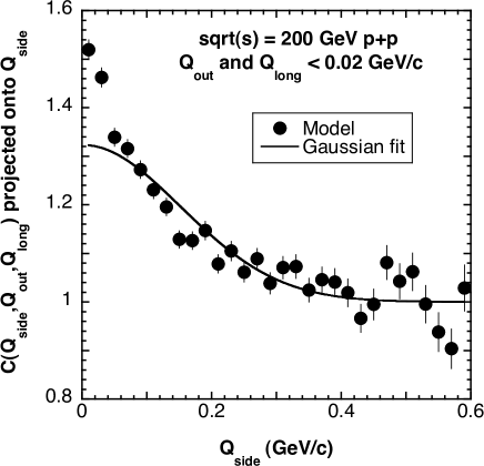
Figure 1: Sample two-pion correlation function with three-dimensional Gaussian fit (Eq.(Signatures for flow effects in $\sqrt{s}=200$ GeV proton-proton collisions.)) projected onto the $Q_{side}$ axis from the Model. The other variables, $Q_{out}$ and $Q_{long}$, are integrated up to 0.02 GeV/c. The cuts on the pion momenta are $-0.5<y<0.5$, $0.15<p_{T}<0.8$ GeV/c, and $0.15<k_{T}<0.25$ GeV/c.

Figure 2 shows the pion momenta and particle multiplicity dependences of the radius parameters from the model, both for the full model calculations (top plots) and for model calculations in which hadronic rescattering is turned off (bottom plots). The pion momenta and particle multiplicity are represented by the quantities $\mathbf{k_{T}}=(\mathbf{p_{T1}}+\mathbf{p_{T2}})/2$ which is the average transverse pion momentum of the pair, and $(1/N)dn/d\eta$ evaluated at $\eta=0$ , which is the (pseudo)rapidity density of charged particles at mid-rapidity, respectively. The dashed lines are fits to the model points, linear for the $k_{T}$-dependence plots and logarithmic for the $(1/N)dn/d\eta$-dependence plots. Focusing on the top two plots first, the full model calculations, it is clear that the radius parameters have the same qualitative dependences on $k_{T}$ and rapidity density as observed in heavy-ion collisions, namely decreasing with increasing $k_{T}$ and increasing with increasing rapidity density (i.e. particle multiplicity). Another trend seen in Figure 2 which is also observed in heavy-ion collisions is $R_{long}>R_{out}>R_{side}$. That hadronic rescattering is the main source of these effects in the model is seen by comparing the top plots with the bottom plots for which rescattering is turned off in the model. In addition to the overall scales of the radius parameters being significantly smaller with rescattering turned off, it is also seen that all of the dependences which were seen in the top plots are either greatly reduced or absent in the bottom plots. A small degree of the $k_{T}$ dependence is seen to linger for $R_{out}$ and $R_{long}$ which is mainly caused by the resonances present in the model.

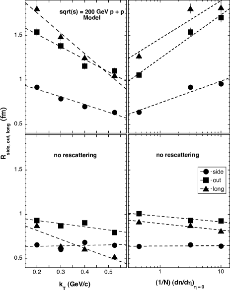
Figure 2: $k_{T}$ and rapidity density dependences of the radius parameters from the model. The top plots show the full model calculations and the bottom plots show model calculations in which hadronic rescattering is turned off. The dashed lines are linear and logarithmic fits to the model points for the $k_{T}$ and rapidity density plots, respectively.

In order to make a more quantitative comparison between the $k_{T}$ dependence seen in Figure 2 in the full model for $p+p$ collisions and that measured in heavy-ion collisions, a calculation has been made of the ratios of the radius parameters extracted in the STAR experiment for $Au+Au$ collisions at $\sqrt{s_{NN}}=200$ GeVAdams:2004yc to those in Figure 2. The same kinematic cuts on the pions as used in Figure 2 were used by the STAR experiment and the STAR results were extracted for a centrality cut of 0-5%. Figure 3 shows a plot of these ratios vs. $k_{T}$. The STAR radius parameters used in calculating the ratios are also plotted. Comparing the $k_{T}$ dependence of the model $p+p$ in the upper left plot of Figure 2 with the STAR radius parameters shown in Figure 3 the qualitative similarity of the plots is evident. As seen, the ratios are approximately flat in $k_{T}$, but with a slight increasing tendency hinting that the decrease of the $p+p$ radius parameters with $k_{T}$ from the model is slightly stronger than that measured in the $Au+Au$ data. Preliminary measurements have been made of radius parameters from $p+p$ collisions at $\sqrt{s}=200$ GeV by STAR and experimental ratios have been calculated as in Figure 3 showing a similarly flat dependence on $k_{T}$ Chajecki:2005zw .

It is difficult to make a quantitative comparison between the model $p+p$ results for the rapidity density shown in Figure 2 and heavy-ion experiments in a similar way as was done for the $k_{T}$ dependence since the range in rapidity density needed to represent the $Au+Au$ measurements is about 100-650, which is much larger than that seen in Figure 2 of 0.3-10. A qualitative comparison can be made in that it can easily be shown that the rapidity density dependence of STAR $Au+Au$ radius parameters from $\sqrt{s_{NN}}=200$ GeV collisions is approximately logarithmically increasing with increasing rapidity density as is seen in Figure 2 Adams:2004yc ; Back:2002wb .

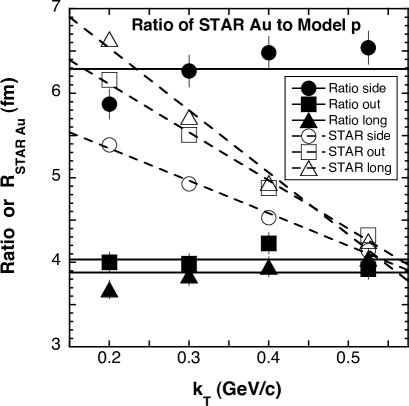
Figure 3: Ratios of STAR $Au+Au$ radius parameters to model $p+p$ radius parameters vs. $k_{T}$. The STAR radius parameters used in calculating the ratios are also plotted. The horizontal solid lines are the averages over $k_{T}$ of the ratios for a given radius parameter. The dashed lines are linear fits to the STAR radius parameters.

In conclusion, it has been shown that flow-like effects observed in relativistic heavy-ion collision experiments can be reproduced in $p+p$ collisions at $\sqrt{s}=200$ GeV by a simple model based on relativistic geometry and final-state hadronic rescattering with a short proper time for hadronization of 0.1 fm/c. In the model, the flow-like effects are driven by the hadronic rescattering which in turn is sensitively controlled by the hadronization time which sets the initial particle density. If a long hadronization time were used, e.g. $\tau=1$ fm/c, the initial particle density would be low and little rescattering would take place such that the full model results would more resemble the bottom plots in Figure 2. Thus to the extent of the agreement shown above between the present model calculations and experiment, another implicit result of this study is that the hadronization time in $p+p$ collisions at this energy appears to be very short.

- (1) I. Arsene et al. [BRAHMS collaboration], Nucl. Phys. A 757, 1 (2005).
- (2) B. B. Back et al. [PHOBOS collaboration], Nucl. Phys. A 757, 28 (2005).
- (3) J. Adams et al. [STAR collaboration], Nucl. Phys. A 757, 102 (2005).
- (4) K. Adcox et al. [PHENIX collaboration], Nucl. Phys. A 757, 184 (2005).
- (5) T. J. Humanic, Int. J. Mod. Phys. E 15, 197 (2006).
- (6) M. A. Lisa, S. Pratt, R. Soltz and U. Wiedemann, Ann. Rev. Nucl. Part. Sci. 55, 357 (2005).
- (7) R. Hanbury Brown and R. Q. Twiss, Nature 177, 27 (1956).
- (8) J. Adams et al. [STAR Collaboration], Phys. Rev. C 71, 044906 (2005).
- (9) T. Sjostrand, L. Lonnblad, S. Mrenna and P. Skands, arXiv:hep-ph/0603175 (March 2006).
- (10) T. Csorgo and J. Zimanyi, Nucl. Phys. A 512, 588 (1990).
- (11) T. J. Humanic, Phys. Rev. C 76, 025205 (2007).
- (12) M. Prakash, M. Prakash, R. Venugopalan and G. Welke, Phys. Rept. 227, 321 (1993).
- (13) W. M. Yao et al. [Particle Data Group], J. Phys. G 33, 1 (2006).
- (14) T. J. Humanic, Phys. Rev. C 73, 054902 (2006).
- (15) T. J. Humanic, Phys. Rev. C 34, 191 (1986).
- (16) T. Alexopoulos et al., Phys. Rev. D 48, 1931 (1993).
- (17) J. L. Bailly et al. [NA23 Collaboration and EHS-RCBC Collaboration], Z. Phys. C 43, 341 (1989).
- (18) Z. Chajecki [STAR Collaboration], Nucl. Phys. A 774, 599 (2006).
- (19) B. B. Back et al., Phys. Rev. Lett. 91, 052303 (2003).