Frequency spectrum of toroidal Alfvén mode in a neutron star with Ferraro’s form of nonhomogeneous poloidal magnetic field

Abstract

Using the energy variational method of magneto-solid-mechanical theory of a perfectly conducting elastic medium threaded by magnetic field, the frequency spectrum of Lorentz-force-driven global torsional nodeless vibrations of a neutron star with Ferraro’s form of axisymmetric poloidal nonhomogeneous internal and dipole-like external magnetic field is obtained and compared with that for this toroidal Alfvén mode in a neutron star with homogeneous internal and dipolar external magnetic field. The relevance of considered asteroseismic models to quasi-periodic oscillations of the X-ray flux during the ultra powerful outbursts of SGR 1806-20 and SGR 1900+14 is discussed.

Keywords Neutron Stars, Asteroseismology, Torsional Alfvén Oscillations

1 Introduction

In the context of recent discovery of quasi-periodic oscillations (QPOs) in the X-ray luminosity during the giant flare of SGR 1806-20 and SGR 1900+14 that were interpreted as being produced by torsional vibrations of quaking magnetars (Israel et al. 2005, Watts & Strohmayer 2006), in (Bastrukov et al. 2009a, 2009b) several scenarios of the post-quake vibrational relaxation of a neutron star model with uniform internal and dipolar external magnetic field

$$B_{r}=B\cos\theta,\quad B_{\theta}=-B\sin\theta,\quad B_{\phi}=0,\quad r\leq R$$ (1)

$$B_{r}=B\left(\frac{R}{r}\right)^{3}\cos\theta,\quad B_{\theta}=-\frac{B}{2}\left(\frac{R}{r}\right)^{3}\sin\theta,\quad B_{\phi}=0,\quad r>R$$ (2)

have been studied on the basis of equations of Newtonian magneto-solid-mechanics

$$\rho{\ddot{\bf u}}=\frac{1}{c}[\delta{\bf j}\times{\bf B}],\quad\delta{\bf j}=\frac{c}{4\pi}[\nabla\times\delta{\bf B}],\quad\delta{\bf B}({\bf r},t)=\nabla\times[{\bf u}\times{\bf B}].$$ (3)

These equations describe the Lorentz-force-driven non-compressional ($\delta\rho=-\rho\nabla\cdot{\bf u}=0$) fluctuations of star matter about axis of above fossil magnetic field ${\bf B}$ in terms of fluctuating material displacements $\bf u$ (the basic dynamical variable of solid mechanics) and the magnetic field $\delta{\bf B}$. It is implied that elastic stellar material is of an extremely high electrical conductivity. The chief argument for interpreting QPOs during the outbursts of above mentioned SGRs (detected on descending branch of the giant flare light-curves) as caused by torsional vibrations of a solid star driven by restoring force of magnetic field stresses is that it is an ultra strong magnetic field frozen-in the entire volume of magnetars serves as the main energy source and promoter of their X-ray bursting seismic activity (e.g., Woods & Thompson 2006, Mereghetti 2008) and, also, bearing in mind the fact that the very notion of torsional vibrations has come into theoretical seismology from the solid-mechanical theory of shear vibrations of an elastic sphere (e.g. Lapwood, & Usami 1981, Lay & Wallace 1995, Aki & Richards 2002, Stein & Wyssesson 2003). It worthy noting that theoretical investigations of non-radial torsional Alfvén oscillations of a fluid star in its own homogeneous magnetic field have a long story that was started, to the best of our knowledge, in works of Jensen (1955) and Plumpton & Ferraro (1955). Remarkably that in the latter paper, by emphasizing the basic discovery of Alfvén that perfectly conducting fluid threaded by magnetic field behaves like anisotropic elastic medium capable of transmitting mechanical disturbance by transverse hydromagnetic waves (e.g. Fälthammar 2007), it is argued that eigenfrequency problem of such vibrations can be tackled on the basis of equation

$$\rho{\ddot{\bf u}}=\frac{1}{4\pi}[\nabla\times[\nabla\times[{\bf u}\times{\bf B}]]]\times{\bf B},\quad\nabla\cdot{\bf u}=0,\quad\nabla\cdot{\bf B}=0$$ (4)

which, as is evident, follows form equations (3). It is clear from this last equation that the frequencies of Alfvén oscillations must substantially depend on both geometrical configuration of internal equilibrium magnetic field ${\bf B}$ and analytic form of oscillating field of material displacements ${\bf u}$. With this obvious observation in mind, in (Bastrukov et al. 2009a, 2009b) focus was laid on non-investigated before regime of large lengthscale nodeless Alfvén oscillations, both global (in the entire spherical volume of star) and crustal (locked in the peripheral finite-depth spherical layer). The most conspicuous feature of this regime is that the radial dependence of oscillating material displacements field ${\bf u}$ has no nodes. In a star undergoing global nodeless torsional oscillations, which are of particular interest for our present discussion, the fluctuating material displacements are described by the toroidal field of the form (Bastrukov et al 2007a, 2007b, 2009a)

$${\bf u}({\bf r},t)=[\mbox{\boldmath$\phi$}({\bf r})\times{\bf r}]\,\alpha(t),\quad\alpha(t)=\alpha_{0}\cos\omega t,$$ (5)

$$\delta{\bf v}({\bf r},t)={\dot{\bf u}}({\bf r},t)=[\delta\mbox{\boldmath$\omega$}({\bf r},t)\times{\bf r}],\quad\delta\mbox{\boldmath$\omega$}({\bf r},t)=\mbox{\boldmath$\phi$}({\bf r})\,{\dot{\alpha}}(t),$$ (7)

$$\mbox{\boldmath$\phi$}({\bf r})=\nabla\chi({\bf r}),\quad\nabla^{2}\chi({\bf r})=0,\quad\chi({\bf r})=\frac{{\cal A}_{\ell}}{\ell+1}\,r^{\ell}\,P_{\ell}(\cos\theta)$$

where $P_{\ell}$ is the Legender polynomial of degree $\ell$ and the other symbols have their usual meaning. Fig.1 illustrates the nodeless character of displacements in the star undergoing global non-radial differentially rotational, torsional, shear vibrations about polar axis in quadrupole and octupole overtones.

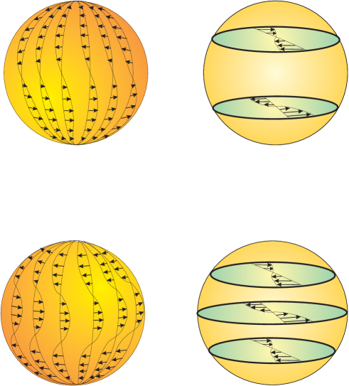
Figure 1: Material displacements in the neutron star undergoing axisymmetric global torsional nodeless vibrations in quadrupole $\ell=2$ and octupole $\ell=3$ overtones.

With the aid of the Rayleigh’s energy method which is expounded below it was found that discrete frequencies of such vibrations is given by the following one-parametric spectral formula (Bastrukov et al. 2009a)

$$\omega(_{0}a^{t}_{\ell})=\omega_{A}\left[(\ell^{2}-1)\frac{2\ell+3}{2\ell-1}\right]^{1/2},\,\,\omega_{A}=\frac{v_{A}}{R}=\sqrt{\frac{RB^{2}}{3M}},$$ (8)

$$\quad v_{A}=\frac{B}{\sqrt{4}\pi\rho},\quad M=\frac{4\pi}{3}\rho\,R^{3}$$ (9)

the only parameter of which is the Alfvén frequency, $\omega_{A}$, of shear magneto-elastic oscillations of perfectly conducting stellar matter matter pervaded by magnetic field $B$ in the star of radius $R$ and mass M. It must be emphasized, however, that this theoretical spectrum does not properly match the QPOs in the X-ray flux from flaring SGR 1806-20 and SGR 1900+14. One of reasons of this discrepancy may be inadequate assumption about homogeneous configuration of internal magnetic field and perhaps the most efficient way to clarify this conjecture is to investigate a model with geometrically different configuration of axisymmetric internal magnetic field. Before so doing it seems worth noting that the model of a star with homogeneous internal and dipolar external magnetic field has come into focus in astrophysics after seminal work of Chandrasekhar and Fermi (1953) in which the effect of mechanical flattening of the star at the poles of such magnetic field has been disclosed. Shortly after, similar conclusion has been drawn in outstanding paper of Ferraro (1954), but on the basis of star model with substantially nonhomogeneous internal and dipole-like axisymmetric poloidal magnetic field

$$B_{r}=\frac{1}{r^{2}\sin\theta}\frac{\partial U}{\partial\theta},\quad B_{\theta}=-\frac{1}{r\sin\theta}\frac{\partial U}{\partial r},\quad B_{\phi}=0,$$ (10)

$$U=U_{in}=\frac{B}{4R^{2}}\,r^{2}(3r^{2}-5R^{2})\sin^{2}\theta,\quad r\leq R,$$ (11)

$$U=U_{ex}=\frac{B}{2r}\,R^{3}\sin^{2}\theta,\quad r>R$$ (12)

where $B$ stands for the magnetic field intensity at the poles and $\nabla\cdot{\bf B}=0$ as should be the case. The meridian cross section of Ferraro’s model of the star is sketched in Fig.2.

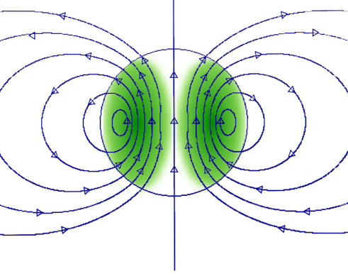
Figure 2: The meridional cross section of a neutron star with Ferraro’s form of inhomogeneous poloidal internal and dipolar external magnetic field whose components are continuous on the star surface, contrary to a highly idealized star model with homogeneous internal and dipolar external magnetic field.

Over the years, the different aspects, both mathematical and astrophysical, of Ferraro’s model have been the subject of extensive investigations (e.g. Chandrasekhar & Prendergast 1955, Robetrs 1955, Chandrasekhar 1956, Mestel 1956, Ledoux & Walraven 1958, Monaghan 1965, Ledoux & Renson 1966, Sood & Trehan 1970, Goossens 1972, Goossens, Smeyers & Denis 1976). The effects of Ferraro’s configuration of magnetic field (and magnetic fields of similar geometrical configuration) on the equilibrium shape, vibrational behavior and electromagnetic activity of pulsars and magnetars are considered in (Roberts 1981, Ioka 2001, Braithwaite & Spruit 2006, Geppert & Rheinhardt 2006, Haskell et al 2008, Lee 2008; Broderick & Narayan 2008, see also references therein).

In this work we focus on the non-studied before regime of global torsional Alfvén nodeless vibrations of neutron star about axis of Ferraro’s magnetic field (10)-(12). In Section 2, the frequency spectrum of this toroidal mode is derived and compared with the frequency spectrum (8) of the neutron star model with homogeneous internal magnetic field. In Section 3, the obtained spectral formula for the frequency is analyzed numerically in juxtaposition with data on QPOs during the flare of SGR 1806-20 and SGR 1900+14. Section 4 briefly accounts for the net outcome of this work. Technical details of analytic computations can be found in Appendix.

2 Global Alfvén torsional nodeless oscillations of neutron star in its own poloidal magnetic field of Ferraro’s form

In the model under consideration a neutron star is identified with a finite spherical mass of an elastic solid, regarded as an incompressible continuous medium of uniform density $\rho$ and an infinite electrical conductivity, whose vibrations under the action of Lorentz magnetic force are governed by equations of magneto-solid-mechanics (2) which can conveniently be represented in the following equivalent tensor form (e.g. Mestel 1999)

$$\rho{\ddot{u}}_{i}=\nabla_{k}\,\delta M_{ik},\quad\delta M_{ik}=\frac{1}{4\pi}[B_{i}\,\delta B_{k}+B_{k}\,\delta B_{i}-(B_{j}\,\delta B_{j})\delta_{ik}],$$ (13)

$$\delta B_{i}({\bf r},t)=(B_{k}\nabla_{k})u_{i}-(u_{k}\nabla_{k})B_{i},\quad\nabla_{i}u_{i}=0$$ (14)

where $\delta M_{ik}$ stands for the Maxwell’s tensor of magnetic field stresses. The energy balance in the process of vibrations is controlled by equation

$$\frac{\partial}{\partial t}\int\frac{\rho{\dot{u}}^{2}}{2}\,d{\cal V}=-\int\delta M_{ik}\,{\dot{u}}_{ik}\,d{\cal V}=-\frac{1}{8\pi}\int[B_{i}\,\delta B_{k}+B_{k}\,\delta B_{i}]\,[\nabla_{i}{\dot{u}}_{k}+\nabla_{k}{\dot{u}}_{i}]\,d{\cal V},$$ (15)

$${\dot{u}}^{2}={\dot{u}}_{i}\,{\dot{u}}_{i},\quad{\dot{u}}_{ik}=\frac{1}{2}[\nabla_{i}{\dot{u}}_{k}+\nabla_{k}{\dot{u}}_{i}],\quad{\dot{u}}_{kk}=\nabla_{k}{\dot{u}}_{k}=0.$$ (16)

To compute the eigenfrequency of toroidal Alfvén mode in question we take advantage of the Rayleigh’s energy method which has been utilized in our previous above mentioned investigations. The key idea of this method consists in separable representation of fluctuating variables such as the vector field of material displacements $u_{i}({\bf r},t)$ and the tensor field of shear strains $u_{ik}({\bf r},t)$

$$u_{i}({\bf r},t)=a_{i}({\bf r})\,{\alpha}(t),\quad u_{ik}({\bf r},t)=a_{ik}({\bf r})\,\,{\alpha}(t),\quad a_{ik}({\bf r})=\frac{1}{2}[\nabla_{i}a_{k}({\bf r})+\nabla_{k}a_{i}({\bf r})].$$ (17)

With this form of $u_{i}$, the magnetic flux density $\delta B_{i}({\bf r},t)$ and the tensor field of fluctuating magnetic field stresses $\delta M_{ik}({\bf r},t)$ are represented in a similar manner

$$\delta B_{i}({\bf r},t)=b_{i}({\bf r})\,\alpha(t),\quad b_{i}({\bf r})=(B_{k}\nabla_{k})a_{i}-(a_{k}\nabla_{k})B_{i},$$ (18)

$$\delta M_{ik}({\bf r},t)=[\tau_{ik}({\bf r})-\frac{1}{2}\tau_{jj}\delta_{ik}]\alpha(t),\quad\tau_{ik}({\bf r})=\frac{1}{4\pi}[B_{i}({\bf r})\,b_{k}({\bf r})+B_{k}({\bf r})\,b_{i}({\bf r})].$$ (19)

The gist of this multiplicative decomposition of fluctuating variables is that on substituting (17)-(19) in (15) this latter equation is reduced to equation for time-dependent amplitude $\alpha(t)$ having the well-familiar form

$${\cal M}{\ddot{\alpha}}(t)+{\cal K}_{m}\alpha(t)=0,\quad{\cal M}=\int\rho\,a_{i}\,a_{i}d{\cal V},$$ (20)

$${\cal K}_{m}=\int\tau_{ik}\,a_{ik}\,d{\cal V}=\frac{1}{8\pi}\int[B_{i}\,b_{k}+B_{k}\,b_{i}]\,[\nabla_{i}\,a_{k}+\nabla_{k}\,a_{i}]\,d{\cal V}.$$ (21)

Thus, from technical argument, the computation of frequency $\omega=[{\cal K}/{\cal M}]^{1/2}$ is reduced to calculation of integral parameters of inertia ${\cal M}$ and stiffness ${\cal K}_{m}$ with the toroidal field of instantaneous, time-independent, displacements

$${\bf a}_{t}=A_{t}\,\nabla\times[{\bf r}\,r^{\ell}\,P_{\ell}(\zeta)]:\,\,a_{r}=0,\,\,\,a_{\theta}=0,\,\,\,a_{\phi}=A_{t}r^{\ell}(1-\zeta^{2})^{1/2}\frac{dP_{\ell}(\zeta)}{d\zeta}$$ (22)

and the magnetic field of Ferraro’s form whose spherical components inside the star are

$$B_{r}=\frac{3B}{2R^{2}}\,r^{2}\left(r^{2}-\frac{5}{3}R^{2}\right)\cos\theta,\quad B_{\theta}=-\frac{3B}{2R^{2}}\,\left(2r^{2}-\frac{5}{3}R^{2}\right)\sin\theta,\quad\quad B_{\phi}=0.$$ (23)

Figure 3: Frequency and period as functions of multipole degree $\ell$ of global torsional Alfvén vibrations of neutron stars with the Ferraro’s shape of internal poloidal magnetic field.

The torsional inertia ${\cal M}$ as a function of multipole degree $\ell$ of nodeless differentially rotational vibrations in question is given by (Bastrukov et al, 2007, 2008)

$${\cal M}=4\pi\rho A_{t}^{2}R^{2\ell+3}\,m_{\ell},\quad m_{\ell}=\frac{\ell(\ell+1)}{(2\ell+1)(2\ell+3)}.$$ (24)

To avoid destructing attention from basic inferences of this work, we place all technical details of tedious but simple computations of integrals for ${\cal K}_{m}$ in Appendix A. The final expression for this coefficient can be represented in the form

$${\cal K}_{m}=B^{2}\,A_{t}^{2}\,R^{2\ell+1}\,k_{\ell},\quad k_{\ell}=\frac{\ell\left(\ell^{2}-1\right)\left(5\ell^{3}+7\ell^{2}+59\ell+84\right)}{2\left(4\ell^{2}-1\right)\left(2\ell+3\right)\left(2\ell+5\right)}.$$ (25)

And for the frequency spectrum of global nodeless torsional Alfvén vibrations nodeless of the neutron star with Ferraro’s form of nonhomogeneous internal magnetic field we obtain

$$\nu(_{0}a^{t}_{\ell})=\nu_{A}\left[\frac{\left(\ell-1\right)\left(5\ell^{3}+7\ell^{2}+59\ell+84\right)}{2\left(2\ell-1\right)\left(2\ell+5\right)}\right]^{1/2},$$ (26)

$$\nu=\frac{\omega}{2\pi},\quad\omega_{A}=\frac{v_{A}}{R},\quad v_{A}=\frac{B}{\sqrt{4\pi\rho}},\quad\omega_{A}=B\sqrt{\frac{R}{3M}},\quad M=\frac{4\pi}{3}\rho\,R^{3}.$$ (27)

It follows that the lowest overtone of this toroidal Alfvén mode is of quadrupole degree, $\ell=2$. At $\ell=1$, the parameter of magneto-mechanical rigidity of neutron star matter cancels, ${\cal K}_{m}(_{0}a^{t}_{1})=0$, and the mass parameter equals to the moment of inertia of rigid sphere, ${\cal M}(_{0}a^{t}_{1})={\cal J}=(2/5)MR^{2}$. It follows from Hamiltonian of normal vibrations, ${\cal H}=(1/2){\cal M}{\dot{\alpha}}^{2}+(1/2){\cal K}{\alpha}^{2}$, that in this dipole case a star sets in rigid-body rotation, rather than vibrations, about axis of its dipole magnetic moment; this feature of the model under consideration is quite similar to that of the neutron star model with homogeneous internal magnetic field. In Fig 3., we plot the frequency $\nu(_{0}a^{t}_{\ell})$ and the period $P(_{0}a^{t}_{\ell})=\nu^{-1}(_{0}a^{t}_{\ell})$ of the Alfvén toroidal mode as functions of multipole degree computed in both homogeneous and nonhomogeneous neutron star models with indicated parameters.

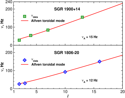
Figure 4: Theoretical fit (lines) of data (symbols) on low-frequency QPOs during the flare of SGRs 1806-20 and 1900+14 by the obtained spectral equation for the toroidal Alfvén oscillations in Ferraro’s poloidal field.

3 QPOs in X-ray luminosity of flaring SGR 1806-20 and SGR 1900+14 from the viewpoint of considered model

As was mentioned, the one-parametric spectral formula (8), computed in the neutron star model with homogeneous internal and dipolar external magnetic field, does not reproduce general trends in data on QPOs frequencies whose numerical values for SGR 1806-20 are given by $\nu_{\rm data}=$18, 26, 30, 92, 150, 625, 1840 and for the SGR 1900+14 these are $\nu_{\rm data}=$28, 54, 84, 155 (Watts & Strohmayer 2007). It is tempting, therefore, to consider these data from the view point of investigated model by identifying the observed QPOs with overtones of spectral formula (26). The result of $\ell$-pole modal specification of the detected QPOs frequencies as overtones of torsional Alfvén seismic vibrations in question is presented in Fig.4 and Fig.5. Specifically, for SGR 1900+14 we obtain: $\nu(_{0}a^{t}_{2})=28$ Hz; $\nu(_{0}a^{t}_{4})=53$; Hz $\nu(_{0}a^{t}_{6})=84$ Hz; $\nu(_{0}t_{13})=155$ Hz, and for the SGR 1806-20 we get $\nu(_{0}a^{t}_{2})=26$ Hz; $\nu(_{0}a^{t}_{3})=30$, $\nu(_{0}a^{t}_{10})=92$ Hz; $\nu(_{0}a^{t}_{16})=155$ Hz; $\nu(_{0}a^{t}_{65})=625$ Hz and $\nu(_{0}a^{t}_{180})=1840$ Hz. While the lowest of detected oscillations, with $\nu=18$ Hz, cannot be specified in terms of considered seismic vibrations, it is clearly seen that the obtained spectrum correctly reflects general trends in the detected QPO frequencies. This suggests, if the detected QPOs are really produced by Lorentz-force-driven global nodeless torsional seismic vibrations about the dipole magnetic moment of magnetars, their internal magnetic fields should be of substantially nonhomogeneous configuration.

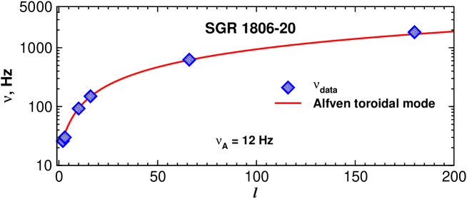
Figure 5: Theoretical fit (lines) of data (symbols) on high-frequency QPOs frequencies during the flare of SGRs 1806-20 by the obtained spectral equation for the frequency of toroidal Alfvén mode.

The result of $\ell$-pole modal specification of the detected QPOs frequencies as overtones of torsional Alfvén seismic vibrations in question is presented in Fig.4 and Fig.5. Specifically, for SGR 1900+14 we obtain: $\nu(_{0}a^{t}_{2})=28$ Hz; $\nu(_{0}a^{t}_{4})=53$; Hz $\nu(_{0}a^{t}_{6})=84$ Hz; $\nu(_{0}t_{13})=155$ Hz, and for the SGR 1806-20 we get $\nu(_{0}a^{t}_{2})=26$ Hz; $\nu(_{0}a^{t}_{3})=30$, $\nu(_{0}a^{t}_{10})=92$ Hz; $\nu(_{0}a^{t}_{16})=155$ Hz; $\nu(_{0}a^{t}_{65})=625$ Hz and $\nu(_{0}a^{t}_{180})=1840$ Hz. While the lowest of detected oscillations, with $\nu=18$ Hz, cannot be specified in terms of considered seismic vibrations, it is clearly seen that the obtained spectrum correctly reflects general trends in the detected QPO frequencies. This suggests, if the detected QPOs are really produced by Lorentz-force-driven global nodeless torsional seismic vibrations about the dipole magnetic moment of magnetars, their internal magnetic fields should be of substantially nonhomogeneous configuration.

4 Concluding remarks

Any attempt to predict the behavior of Alfvén vibrational modes in pulsars and magnetars, presuming of course that the star material possesses properties of perfectly conducting continuous medium pervaded by magnetic fields, is beset with uncertainties regarding geometrical configuration of fossil internal magnetic field. It seems, therefore, that progress can be best made by studying these modes within the framework of comprehensive models. Among these are the models with homogeneous and nonhomogeneous axisymmetric poloidal magnetic fields considered long ago in works of Chandrasekhar and Fermi (1953) and by Ferraro (1954), respectively, to show that such fields have the same effect as rigid rotation, that is, tend to produce a flattening of the star shape along the magnetic field axis. Following this line of argument and continuing investigations reported in (Bastrukov et al 2009a), we have computed here the frequency spectrum of axisymmetric torsional nodeless vibrations, in the neutron star model with Ferraro’s form of nonhomogeneous poloidal magnetic field which is presented in Fig.3 in juxtaposition in a neutron star model with homogeneous internal field.

The practical usefulness of the obtained one-parametric spectral formula has been demonstrated by its application to $\ell$-pole identification of QPOs frequencies during the X-ray giant outbursts of SGR 1900+14 and SGR 1806-20. The result of our analysis, summarized in Fig.4 and Fig.5, shows that the model adequately regains the overall trends in the detected QPOs frequencies and, thus, supports theoretical interpretation of these QPOs, advanced in works reporting this discovery (Israel et al 2005, Watts & Strohmayer 2006), as owing their origin to quake-induced torsional seismic vibrations of underlying magnetar. Together with this, in (Bastrukov et al 2009b) it has been shown that the same data on the QPO frequencies can be consistently interpreted from the view point of two-component, core-crust, model of quaking neutron star (Franco et al. 2000) with homogeneous internal magnetic field as being produced by axisymmetric differentially rotational Alfvén nodeless oscillations of crustal solid-state plasma about axis of magnetic field frozen in the immobile core. With all these in mind, we conclude that it is the Lorentz force of magnetic field stresses plays decisive part in post-quake vibrational relaxation of above magnetars and that the toroidal fields of quake-induced material displacements are of substantially nodeless character.

Authors are grateful to Dr. Dima Podgainy for helpful assistance. This work has been supported by NSC of Taiwan, grant numbers NSC-098-2811-M-007-009 and NSC-96-2628-M-007-012-MY3.

Appendix A Torsional stiffness of global torisonal Alfvén nodeless oscillations of a neutron star about axis of Ferraro’s nonhomogeneous poloidal magnetic field

In computing stiffness of torsional Alfvén oscillations

$${\cal K}_{m}=\int\tau_{ik}({\bf r})\,a_{ik}({\bf r})\,d{\cal V},\quad a_{ik}({\bf r})=\frac{1}{2}[\nabla_{i}\,a_{k}({\bf r})+\nabla_{k}\,a_{i}({\bf r})],$$

$$\tau_{ik}({\bf r})=\frac{1}{4\pi}[B_{i}({\bf r})\,b_{k}({\bf r})+B_{k}\,({\bf r})b_{i}({\bf r})],\quad b_{i}({\bf r})=(B_{k}({\bf r})\nabla_{k})a_{i}({\bf r})-(a_{k}({\bf r})\nabla_{k})B_{i}({\bf r})$$

it is convenient to represent strain tensor

$$a_{ik}=\frac{1}{2}(\nabla_{i}a_{k}+\nabla_{k}a_{i})$$

in spherical polar coordinates with use of the angle variable ${\zeta}=\hbox{cos}\,{\theta}$. In terms of this variable, the components of these tensor are

$$a_{rr}=\frac{\partial a_{r}}{\partial r},\quad\quad\quad a_{\theta\theta}=-\frac{(1-\zeta^{2})^{1/2}}{r}\frac{\partial a_{r}}{\partial\zeta}+\frac{a_{r}}{r},$$

$$a_{\phi\phi}=\frac{1}{r}\frac{1}{(1-\zeta^{2})^{1/2}}\frac{\partial{a_{\phi}}}{\partial{\phi}}+\frac{a_{r}}{r}+\frac{\zeta}{(1-\zeta^{2})^{1/2}}\frac{a_{\theta}}{r},$$

$$a_{r\theta}=\frac{1}{2}\left[-\frac{(1-\zeta^{2})^{1/2}}{r}\frac{\partial a_{r}}{\partial\zeta}-\frac{a_{\theta}}{r}+\frac{\partial a_{\theta}}{\partial r}\right],$$

$$a_{r\phi}=\frac{1}{2}\left[\frac{1}{r}\frac{1}{(1-\zeta^{2})^{1/2}}\frac{\partial a_{r}}{\partial\phi}-\frac{a_{\phi}}{r}+\frac{\partial a_{\phi}}{\partial r}\right],$$

$$a_{\theta\phi}=\frac{1}{2}\left[\frac{1}{r}\frac{1}{(1-\zeta^{2})^{1/2}}\frac{\partial a_{\theta}}{\partial\phi}-\frac{\zeta}{(1-\zeta^{2})^{1/2}}\frac{a_{\phi}}{r}-\frac{(1-\zeta^{2})^{1/2}}{r}\frac{\partial a_{\phi}}{\partial\zeta}\right].$$

In the torsional mode of nodeless vibrations the field of instantaneous displacements has solely one non-zero $\phi-th$ component

$$a_{r}=0\quad a_{\theta}=0\quad a_{\phi}=A_{t}\,r^{\ell}(1-\zeta^{2})^{1/2}P^{\prime}_{\ell}(\zeta),\quad P^{\prime}_{\ell}(\zeta)=\frac{dP_{\ell}(\zeta)}{d\zeta}.$$

In this case we have only two non-zero components of the strain tensor

$$a_{rr}=a_{\theta\theta}=a_{\phi\phi}=a_{r\theta}=0,$$

$$a_{r\phi}=\frac{A_{t}}{2}r^{\ell-1}(\ell-1)(1-\zeta^{2})^{1/2}P^{\prime}_{\ell},\quad a_{\theta\phi}=-\frac{A_{t}}{2}r^{\ell-1}\left[2\zeta P^{\prime}_{\ell}-\ell(\ell+1)P_{\ell}(\zeta)\right].$$

In spherical polar coordinates the components of vector field $b_{i}({\bf r})=(B_{k}\nabla_{k})a_{i}-(a_{k}\nabla_{k})B_{i}$ are given by

$$b_{r} = \left[B_{r}\frac{\partial}{\partial r}-\frac{B_{\theta}}{r}(1-\zeta^{2})^{1/2}\frac{\partial}{\partial\zeta}+\frac{B_{\phi}}{r}(1-\zeta^{2})^{-1/2}\frac{\partial}{\partial\phi}\right]\,a_{r}-\frac{B_{\theta}\,a_{\theta}+B_{\phi}\,a_{\phi}}{r}$$

$$- \left[a_{r}\frac{\partial}{\partial r}-\frac{a_{\theta}}{r}(1-\zeta^{2})^{1/2}\frac{\partial}{\partial\zeta}+\frac{a_{\phi}}{r}(1-\zeta^{2})^{-1/2}\frac{\partial}{\partial\phi}\right]\,B_{r}+\frac{a_{\theta}\,B_{\theta}+a_{\phi}\,B_{\phi}}{r},$$

$$b_{\theta} = \left[B_{r}\frac{\partial}{\partial r}-\frac{B_{\theta}}{r}(1-\zeta^{2})^{1/2}\frac{\partial}{\partial\zeta}+\frac{B_{\phi}}{r}(1-\zeta^{2})^{-1/2}\frac{\partial}{\partial\phi}\right]\,a_{\theta}+\frac{B_{\theta}\,a_{r}-B_{\phi}\,a_{\phi}\,\zeta(1-\zeta^{2})^{-1/2}}{r}$$

$$- \left[a_{r}\frac{\partial}{\partial r}-\frac{a_{\theta}}{r}(1-\zeta^{2})^{1/2}\frac{\partial}{\partial\zeta}+\frac{a_{\phi}}{r}(1-\zeta^{2})^{-1/2}\frac{\partial}{\partial\phi}\right]\,B_{\theta}-\frac{a_{\theta}\,B_{r}-a_{\phi}\,B_{\phi}\,\zeta(1-\zeta^{2})^{-1/2}}{r},$$

$$b_{\phi} = \left[B_{r}\frac{\partial}{\partial r}-\frac{B_{\theta}}{r}(1-\zeta^{2})^{1/2}\frac{\partial}{\partial\zeta}+\frac{B_{\phi}}{r}(1-\zeta^{2})^{-1/2}\frac{\partial}{\partial\phi}\right]\,a_{\phi}+\frac{B_{\phi}\,a_{r}+B_{\phi}\,a_{\theta}\,\zeta(1-\zeta^{2})^{-1/2}}{r}$$

$$- \left[a_{r}\frac{\partial}{\partial r}-\frac{a_{\theta}}{r}(1-\zeta^{2})^{1/2}\frac{\partial}{\partial\zeta}+\frac{a_{\phi}}{r}(1-\zeta^{2})^{-1/2}\frac{\partial}{\partial\phi}\right]\,B_{\phi}-\frac{a_{\phi}\,B_{r}+a_{\phi}\,B_{\theta}\,\zeta(1-\zeta^{2})^{-1/2}}{r}.$$

Taking into account that Ferraro’s field has only two non-zero components which can be conveniently represented in the form

$$B_{r}=\frac{2f}{r^{2}}\,\zeta,\quad B_{\theta}=-\frac{(1-\zeta)^{1/2}}{r}\,f^{\prime},\quad B_{\phi}=0,\quad f=\frac{B}{4R^{2}}\,r^{2}(3r^{2}-5R^{2}),\quad f^{\prime}=\frac{df}{dr}$$

for the components of $b_{i}$ we obtain

$$b_{r}=0,\quad b_{\theta}=0,\quad b_{\phi}=B_{r}\frac{\partial a_{\phi}}{\partial r}-\frac{B_{\theta}}{r}(1-\zeta^{2})^{1/2}\frac{\partial a_{\phi}}{\partial\zeta}-\frac{a_{\phi}\,B_{r}}{r}-\frac{a_{\phi}\,B_{\theta}\,\zeta(1-\zeta^{2})^{-1/2}}{r}$$

where

$$\frac{\partial a_{\phi}}{\partial r} = A_{t}\,\ell\,r^{\ell-1}(1-\zeta^{2})^{1/2}P^{\prime}_{\ell},\quad\quad\frac{\partial a_{\phi}}{\partial\zeta}=A_{t}\,r^{\ell}\,\left(1-\zeta^{2}\right)^{-1/2}\left[\zeta\,P^{\prime}_{\ell}-\ell\left(\ell+1\right)\right].$$

The integrand of ${\cal K}_{m}$ reads

$$\tau_{ik}a_{ik}=2\left(\tau_{r\phi}a_{r\phi}+\tau_{\theta\phi}a_{\theta\phi}\right)$$

so that relevant to computation of ${\cal K}_{m}$ components of tensor $\tau_{ik}=(1/4\pi)[B_{i}\,b_{k}+B_{k}\,b_{i}]$ are given by

$$\tau_{r\phi} = \frac{1}{4\pi}\left[B_{r}B_{r}\frac{\partial a_{\phi}}{\partial r}-\frac{B_{r}B_{\theta}}{r}(1-\zeta^{2})^{1/2}\frac{\partial a_{\phi}}{\partial\zeta}\,-\frac{a_{\phi}\,B_{r}B_{r}}{r}-\frac{a_{\phi}\,B_{r}B_{\theta}\,\zeta(1-\zeta^{2})^{-1/2}}{r}\right]$$

$$= \frac{A_{t}}{4\pi}\left\{4(\ell-1)f^{2}r^{\ell-5}\zeta^{2}(1-\zeta^{2})^{1/2}P^{\prime}_{\ell}+2ff^{\prime}r^{\ell-4}\zeta(1-\zeta^{2})^{1/2}[2\zeta P^{\prime}_{\ell}-\ell(\ell+1)P_{\ell}]\right\},$$

$$\tau_{\theta\phi} = \frac{1}{4\pi}\left[B_{\theta}B_{r}\frac{\partial a_{\phi}}{\partial r}-\frac{B_{\theta}B_{\theta}}{r}(1-\zeta^{2})^{1/2}\frac{\partial a_{\phi}}{\partial\zeta}\,-\frac{a_{\phi}\,B_{\theta}B_{r}}{r}-\frac{a_{\phi}\,B_{\theta}\,B_{\theta}\,\zeta(1-\zeta^{2})^{-1/2}}{r}\right]$$

$$= \frac{A_{t}}{4\pi}\left[-2r^{\ell-4}\left(\ell-1\right)ff^{\prime}\zeta\left(1-\zeta^{2}\right)P^{\prime}_{\ell}-r^{\ell-3}f^{\prime 2}\left(1-\zeta^{2}\right)\left[2\zeta P^{\prime}_{\ell}-\ell\left(\ell+1\right)P_{\ell}\right]\right].$$

The integral for stiffness can be conveniently represented in the form

$${\cal K}_{m} = 2\int[\tau_{r\phi}\,a_{r\phi}+\tau_{\theta\phi}\,a_{\theta\phi}]d{\cal V}=\frac{A_{t}^{2}}{2}\left\{4(\ell-1)^{2}R_{ff}I_{1}+4(\ell-1)R_{ff^{\prime}}[2I_{1}-\ell(\ell+1)I_{2}]\right.$$

$$+ \left.R_{f^{\prime}f^{\prime}}[4I_{1}-4\ell(\ell+1)I_{2}+\ell^{2}(\ell+1)^{2}I_{3}]\right\}$$

The integrals $I_{i}$ are computed with aid of standard recurrence relations between Legendre polynomials (e.g. Abramowitz & Stegan 1964) which yield

$$I_{1}=\int\limits_{-1}^{1}\zeta^{2}(1-\zeta^{2})(P^{\prime}_{\ell})^{2}d\zeta=\frac{2\,\ell\,(\ell+1)(2\ell^{2}+2\ell-3)}{(4\ell^{2}-1)(2\ell+3)},$$

$$I_{2}=\int\limits_{-1}^{1}\zeta(1-\zeta^{2})P_{\ell}\,P^{\prime}_{\ell}d\zeta=\frac{2\,\ell\,(\ell+1)}{(4\ell^{2}-1)(2\ell+3)},$$

$$I_{3}=\int\limits_{-1}^{1}(1-\zeta^{2})P_{\ell}^{2}d\zeta=\frac{4\,(\ell^{2}+\ell-1)}{(4\ell^{2}-1)(2\ell+3)},\quad I_{4}=\int\limits_{-1}^{1}\zeta^{2}(1-\zeta^{2})P_{\ell}P^{\prime}_{\ell}d\zeta=\,0.$$

For integrals with function $f=(B/4R^{2})[r^{2}(3r^{2}-5R^{2})]$ we obtain

$$R_{ff}=\int_{0}^{R}f^{2}(r)r^{2\ell-4}dr=\frac{B^{2}R^{2\ell+1}}{16}R_{1},\quad R_{1}=\left[\frac{25}{2\ell+1}-\frac{30}{2\ell+3}+\frac{9}{2\ell+5}\right],$$

$$R_{ff^{\prime}}=\int_{0}^{R}f\left(\frac{df}{dr}\right)r^{2\ell-3}dr=\frac{B^{2}R^{2\ell+1}}{16}R_{2},\quad R_{2}=\left[\frac{50}{2\ell+1}-\frac{90}{2\ell+3}+\frac{36}{2\ell+5}\right],$$

$$R_{f^{\prime}f^{\prime}}=\int_{0}^{R}\left(\frac{df}{dr}\right)^{2}r^{2\ell-2}dr=\frac{B^{2}R^{2\ell+1}}{16}R_{3},\quad R_{3}=\left[\frac{100}{2\ell+1}-\frac{240}{2\ell+3}+\frac{144}{2\ell+5}\right].$$

The resultant expression for the stiffness reads

$${\cal K}_{m}=B^{2}\,A_{t}^{2}\,R^{2\ell+1}\,k_{\ell}$$

where

$$k_{\ell} = \frac{1}{32}\left\{4(\ell-1)^{2}R_{1}\,I_{1}+4(\ell-1)R_{2}[2I_{1}-\ell(\ell+1)I_{2}]+R_{3}[4I_{1}-4\ell(\ell+1)I_{2}+\ell^{2}(\ell+1)^{2}I_{3}]\right\}$$

$$= \frac{\ell\left(\ell^{2}-1\right)}{2\left(4\ell^{2}-1\right)\left(2\ell+3\right)\left(2\ell+5\right)}\left(5\ell^{3}+7\ell^{2}+59\ell+84\right).$$

References

- (1) Abramowitz M. & Stegan I.A. 1964, Handbook of Mathematical Functions. Dover, New York
- (2) Aki K. & Richards P. G., 2002, Quantitative Seismology. University Science Books
- (3) Bastrukov, S. I., Chang, H.-K., Mişicu, Ş., Molodtsova, I. V. & Podgainy D. V. 2007a, Int. J. Mod. Phys. A, 22, 3261
- (4) Bastrukov, S. I., Chang, H.-K., Takata, J., Chen, G.-T. & Molodtsova I. V. 2007b, MNRAS, 382, 849
- (5) Bastrukov, S. I., Chang, H.-K., Chen, G.-T. & Molodtsova I. V. 2008, Mod. Phys. Lett. A., 23, 477
- (6) Bastrukov, S. I., Chen, G.-T., Chang H.-K., Molodtsova, I. V., Podgainy, D. V. 2009a, ApJ, 690, 998
- (7) Bastrukov, S. I., Chang, H.-K., Molodtsova I. V. & , Takata, J., 2009b, arXiv e-prints, 0812.4524
- (8) Bhattacharya, D. & van den Heuvel E. P. J. 1991, Phys. Rep., 2003, 1
- (9) Braithwaite, J. & Spruit, H. C. 2006, A&A, 450, 1097
- (10) Broderick, A. E. & Narayan, R. 2008, MNRAS, 383, 943
- (11) Chandrasekhar, S. & Fermi 1953, ApJ, 118, 116
- (12) Chandrasekhar, S. & Prendergast K. H. 1955, PNAS, 42, 5
- (13) Chandrasekhar, S. 1956, ApJ, 124, 232
- (14) Chandrasekhar, S. 1961, Hydromagnetic and Hydrodynamic Stability. Oxford University Press
- (15) Chanmugam, G. 1992, , 65, 301
- (16) Geppert, U. & Rheinhardt, M. 2006, A&A, 456, 639
- (17) Goldreich, P. & Reisenegger, A. 1992, ApJ, 395, 250
- (18) Goossens M., 1972, A&SS, 16, 386
- (19) Goossens M., Smeyers P. & Denis J., 1976, A&SS, 39, 257
- (20) Haskell, B., Samuelsson, L., Glampedakis, K. & Andersson, N. 2008, MNRAS, 385, 531
- (21) Jensen, E., 1955, ApJS, 2, 141
- (22) Fälthammar, C.-G., 2007, JASTP, 69, 1604
- (23) Ferraro, V.C.A., 1954, ApJ, 119, 407
- (24) Franco, L. M., Link B. & Epstein R. I. 2000, ApJ, 543, 987
- (25) Israel, G. L., Belloni, T., Stella, L., Rephaeli Y., Gruber, D. E., Casella, P., Dall’Osso, S., Rea, N., Persic, M. & Rothschild R. E. 2005, ApJ, 628, L53
- (26) Ioka, K. 2001, MNRAS, 327, 639
- (27) Lapwood, R. R. & Usami T., 1981, Free Oscillations of the Earth. Cambridge Univ. Press
- (28) Lay, T. & Wallace, T.C. 1995, Modern global seismology. Volume 58 of International geophysics series. Academic Press, San Diego
- (29) Ledoux, P. & Walraven, T. H. 1958, Handb. Der. Phys., 51, Ed. Flugge S., Springer, p.353
- (30) Ledoux, P. & Renson, P. 1966, ARA&A, 4, 293
- (31) Lee, U. 2008, MNRAS, 385, 2069
- (32) Mestel, L. 1956, MNRAS, 116, 324
- (33) Mestel, L. 1999, Stellar Magnetism. Clarendon Press, Oxford
- (34) Monaghan, J. J. 1965, MNRAS, 131, 105
- (35) Mereghetti, S. 2008, A&ARv, 15, 225
- (36) Plumpton, C. & Ferraro, V. C. A. 1955, ApJ, 121, 168
- (37) Roberts, P. H. 1955, ApJ, 112, 508
- (38) Roberts, P. H. 1981, AN, 302, 65
- (39) Sood N. K. & Trehan S. K., 1970, A&SS, 10, 393
- (40) Stein S. & Wyssesson M., 2003, An Introduction to Seismology, Earthquakes, and Earth structure. Blackwell, Oxford
- (41) Watts, A. L. & Strohmayer T. E. 2006, ApJ, 637, L117
- (42) Watts, A. L. & Strohmayer T. E. 2007, AdSpR, 40, 144
- (43) Woods, P. M. & Thompson, C. 2006, in Compact Stellar X-ray Sources, ed. Lewin, W. & van der Klis, M. (Cambridge: Cambridge University Press)