An effective method to estimate multidimensional Gaussian states

Abstract

A simple and efficient method for characterization of multidimensional Gaussian states is suggested and experimentally demonstrated. Our scheme shows analogies with tomography of finite dimensional quantum states, with the covariance matrix playing the role of the density matrix and homodyne detection providing Stern-Gerlach-like projections. The major difference stems from a different character of relevant noises: while the statistics of Stern-Gerlach-like measurements is governed by binomial statistics, the detection of quadrature variances correspond to $\chi^{2}$ statistics. For Gaussian and near Gaussian states the suggested method provides, compared to standard tomography techniques, more stable and reliable reconstructions. In addition, by putting together reconstruction methods for Gaussian and arbitrary states, we obtain a tool to detect the non-Gaussian character of optical signals.

I Introduction

Gaussian states are building blocks of quantum information processing with continuous variables. In fact, Gaussian states can be generated and processed by means of linear operations. On the other hand, successful implementation of quantum information protocols requires efficient tools for the analysis and characterization of the quantum states involved in the experiment LNP . The standard approach to characterize optical continuous variables states is to perform homodyne measurements firsthomodyne and reconstruct the measured quantum state on a subspace of the infinitely dimensional space describing a multi-mode quantum harmonic oscillator vogel . This approach is rather general and, in principle, can be used for reconstructing both Gaussian firsthomodyne ; squeezedcoherent ; gaussian ; CovMat ; CMs and non-Gaussian onephoton ; grg ; polzik states. On the other hand, such a general procedure becomes inherently inefficient once the set of possible states is restricted. For example, the knowledge about the Gaussian character of the measured state contributes a lot of prior information about the measured subject. This information can be used for reducing the number of relevant unknown parameters, making the reconstruction (data inversion) much simpler, also avoiding problematic issues of the standard approach, such as the rapid growth of reconstruction errors with the size of the reconstruction space chyby ; qt .

The main idea of the present contribution is to point out and exploit formal analogies between the description of Gaussian states and that of finite-dimensional quantum states. Based on this analogy we put forward a simple and efficient method for reconstructing Gaussian states from homodyne data. Since by definition the result of Gaussian tomography is a Gaussian state, the quality of Gaussian fit can also be used to assess how far is the measured state from the family of Gaussian states, thus providing an operational definition of Gaussianity for quantum states nonG . This will be demonstrated upon the application of the method to homodyne data taken on states produced by an optical parametric oscillator close to threshold solimeno .

The paper is structured as follows. In Section II we review few basics facts related to Gaussian states and homodyne detection. This will be used in Section III for the formulation of a reconstruction method based on the detection of rotated field-quadrature operator. The theory is then generalized to multidimensional Gaussian states in Section IV. Experimental results and data analysis are reported in in Sec. V, whereas Section VI closes the paper with some concluding remarks.

II Homodyning Gaussian states

For the sake of simplicity we start by formulating the problem of reconstruction for single mode Gaussian field $\varrho$, with Wigner function given by

$$W(\bm{X})=\frac{\exp\left\{-\frac{1}{2}{(\bm{X}-\overline{\bm{X}})^{T}\bm{G}^{-1}(\bm{X}-\overline{\bm{X}})}\right\}}{2\pi\sqrt{{\rm Det}[\bm{G}]}}\>,$$ (1)

with $\bm{X}^{T}=(x,y)$ and covariance matrix $\bm{G}$ given by

$$\bm{G}\equiv\frac{1}{2}\begin{pmatrix}2(\Delta X)^{2}&\{\Delta X,\Delta Y\}\\ \{\Delta X,\Delta Y\}&2(\Delta P)^{2}\end{pmatrix}\geq{\bm{\Omega}}\equiv\frac{1}{2}\begin{pmatrix}0&-i\\ i&0\end{pmatrix}\,.$$ (2)

where $X=(a+a^{\dagger})/\sqrt{2}$ and $Y=i(a^{\dagger}-a)/\sqrt{2}$, are the quadrature operators, $a$ and $a^{{\dagger}}$ being mode operators. If the homodyne detector is set to measure the quadrature $X(\theta)=X\cos\theta+Y\sin\theta$, the positive operator valued measure (POVM) $\Pi_{\eta}(x,\theta)$ associated with its realistic measurement is the Gaussian convolution of the quadrature projectors,

$$\Pi_{\eta}(x,\theta)=\int\frac{dy}{\sqrt{2\pi\delta_{\eta}^{2}}}\>\exp\left\{-\frac{(y-\frac{x}{\sqrt{\eta}})^{2}}{2\delta_{\eta}^{2}}\right\}\>|y\rangle_{\phi}{}_{\phi}\langle y|,$$ (3)

where $\delta_{\eta}^{2}=(1-\eta)/2\eta$, and $\eta$ is the quantum efficiency of the involved (linear) photodetectors. In the Fock basis we have

$$|y\rangle_{\phi}=\left(\frac{1}{\pi}\right)^{1/4}e^{-\frac{1}{2}y^{2}}\sum_{k=0}^{\infty}\frac{H_{k}(y)}{2^{k/2}\sqrt{k!}}e^{-ik\phi}|k\rangle\,,$$ (4)

and the distribution of homodyne outcomes is given by

$$p_{\eta}(x,\theta) ={\rm Tr}\left[\varrho\>\Pi_{\eta}(x,\theta)\right]$$ (5)

$$=\frac{\exp\left\{-\left(x-\left[{\bm{R}}_{\theta}\overline{\bm{X}}\right]_{1}\right)^{2}/(2\,\sigma^{2}_{\eta})\right\}}{\sqrt{2\pi\,\sigma^{2}_{\eta}}}\,,$$ (6)

where $\sigma^{2}_{\eta}=\eta(M_{22}{\rm Det}[\bm{G}]+\delta_{\eta}^{2})$, $M_{22}=[\bm{M}]_{22}$, with $\bm{M}={\bm{R}}_{\theta}\,\bm{G}^{-1}\bm{R}_{-\theta}$, and the rotation matrix is defined as

$$\bm{R}_{\theta}=\begin{pmatrix}\cos\theta&\sin\theta\\ -\sin\theta&\cos\theta\end{pmatrix}\,.$$

III Estimation of covariance matrix

In this Section, we address the problem how to estimate efficiently the covariance matrix $\bm{G}$. For the sake of simplicity let us set the coherent part of the signal to zero and $\eta=1$. Introducing a unit vector $\langle\bm{u}|=(\cos{\theta},\sin{\theta})$ parametrized by the phase of the local oscillator and noticing that $\langle\bm{u}|\bm{G}|\bm{u}\rangle=M_{22}{\rm Det}[\bm{G}]$, the sampled probability density (6) may be conveniently expressed in the form

$$p(x,\theta)=\frac{1}{\sqrt{2\pi\,\langle\bm{u}|\bm{G}|\bm{u}\rangle}}\exp\left\{-\frac{x^{2}}{2\,\langle\bm{u}|\bm{G}|\bm{u}\rangle}\right\}\,.$$ (7)

There are several striking similarities between the reconstruction of spin $1/2$ states and covariance matrices. Indeed, in both cases the state is described by $2\times 2$ matrices. The density matrix of the spin $1/2$ state is a hermitian, unit trace, semi-positive matrix, thus leaving three free parameters for its full description. The covariance matrix is real, symmetric matrix, again fully described by three parameters, constrained to the relation (2). Projections of a spin density matrix are conveniently sampled in a Stern-Gerlach experiment. Similarly, detections of quadrature variables in a homodyne experiment provide sampling of quadrature variances representing projections of a covariance matrix. Indeed, estimated matrix $\bm{G}$ appears only in the variance of distribution (7). Single detected event do not say too much, but repeated detections do. Provided that homodyne detection is repeated $n$ times for the same setting, $x_{i}$ being the detected results, the likelihood of $\bm{G}$ reads

$${\cal L}(\bm{G}|\{x_{i}\})\propto\frac{1}{(2\pi\,\langle\bm{u}|\bm{G}|\bm{u}\rangle)^{n/2}}\exp\left\{-\frac{\sum_{i}x_{i}^{2}}{2\,\langle\bm{u}|\bm{G}|\bm{u}\rangle}\right\}.$$ (8)

Consider now the statistics of the random variable

$$y=\sum_{k}x_{i}^{2},$$

which is given by

$$P_{G}(y)=\int dx_{1}\ldots dx_{n}\delta(y-\sum_{i}x_{i}^{2}){\cal L}(\bm{G}|\{x_{i}\}).$$ (9)

It is easy to see that for Gaussian states the fluctuations of $y$ variable are governed by the well-known $\chi^{2}$ distribution

$$P_{G}(y)=\frac{2^{-n/2}}{\Gamma(n/2)}\frac{y^{n/2-1}}{\big{[}\sigma^{2}(\bm{G})\big{]}^{n/2}}\exp\left\{-\frac{y}{2\,\sigma^{2}(\bm{G})}\right\}.$$ (10)

Upon maximizing the likelihood (10), the quadrature variance, which plays the role of a projection of the covariance matrix, $\sigma^{2}(\bm{G})=\langle\bm{u}|\bm{G}|\bm{u}\rangle$, is estimated as

$$\sigma^{2}(\bm{G})=\frac{1}{n}\sum_{i}x_{i}^{2}.$$ (11)

This establishes a formal analogy between estimations of spin states and Gaussian covariance matrices. In the former case the probability of finding the spin “up” is sampled by the number of particles deflected upwards in a Stern-Gerlach apparatus. Similarly, for Gaussian states the variance of a quadrature distribution (i.e. a projection of the covariance matrix) is sampled by properly normalized sum of squares of the detected quadrature values.

Having mentioned similarities between the two problems let us also identify three important differences between the estimation of a spin $1/2$ system and estimation of a Gaussian state:

1. the two problems have different underlying statics: binomial statistics for yes-no spin data and $\chi^{2}$ distribution for sampled variances;

2. there are slightly different constraints on the estimated quantities: semi-positivity of density matrix for spins and uncertainty relations constraint, stated in the form of the matrix inequality (2), for Gaussian states;

3. the measured quantities have different nature: for spins the sampled probabilities are expectation values of Stern-Gerlach outcomes whereas for Gaussian states we need sampled variances of the homodyne data, i.e the information is contained in the data noise.

Notice that properties (ii) and (iii) will be important for the discussion of our main result below.

In order to get a unique reconstruction of the measured Gaussian state, quadrature measurement should be repeated with different settings of phases $\theta_{h}$ of the strong local oscillator. Let us assume that each quadrature $X(\theta_{h})$ is sampled $n_{h}$ times with the results $x_{h,1},\,x_{h,2},\ldots x_{h,n_{h}}$, and denote $y_{h}=\sum_{k}x_{h,k}^{2}$. The corresponding log-likelihood reads

$$\log{\cal L}(\bm{G})=-\frac{1}{2}\sum_{h}n_{h}\log\sigma_{h}^{2}(\bm{G})-\sum_{h}\frac{y_{h}}{2\,\sigma_{h}^{2}(\bm{G})}\,,$$ (12)

where $\sigma_{h}^{2}(G)=\langle\bm{u}_{h}|\bm{G}|\bm{u}_{h}\rangle$. A reconstruction of the signal covariance matrix is then obtained by maximizing the likelihood function subject to the constraint $\bf G\geq\Omega$. Let us first consider the extremal equation for the covariance matrix. It is easily found by taking a derivative of $\log{\cal L}(\bm{G})$ with respect to matrix $\bm{G}$. This yields

$$R\bm{G}=D\bm{G},$$ (13)

where

$$D =\sum_{h}\frac{n_{h}}{\langle\bm{u}_{h}|\bm{G}|\bm{u}_{h}\rangle}|\bm{u}_{h}\rangle\langle\bm{u}_{h}|\,,$$ (14)

$$R =\sum_{h}\frac{y_{h}}{\langle\bm{u}_{h}|\bm{G}|\bm{u}_{h}\rangle^{2}}|\bm{u}_{h}\rangle\langle\bm{u}_{h}|.$$ (15)

As there is again a direct analogy between the extremal equation for $\bm{G}$ and the corresponding extremal equation for the maximum-likely spin state, methods developed for generic quantum estimation can be employed, with some caution, to solve the extremal equation (13) by iterations mylvovsky . A form suitable to iterations can be found noting that by Hermicity of $\bm{G}$, $R$ and $D$ both $\bm{G}=D^{-1}R\bm{G}$ and $\bm{G}=\bm{G}RD^{-1}$ simultaneously hold and may be combined into a single extremal matrix equation

$$\bm{G}=D^{-1}R\bm{G}RD^{-1},$$ (16)

which is our main formal result. This matrix equation may be iterated starting e.g. with the covariance matrix of the vacuum state. In addition the form of Eq. (16) guarantees that semi-positivity, $\bm{G}\geq 0$, of the covariance matrix is preserved after each iteration step.

Some discussion of this algorithm is now in order. As we have already mentioned above condition $\bm{G}\geq 0$ would be typical for density matrices. Covariance matrices obey a more complicated relation $\bm{G}\geq\bm{\Omega}$. Though in principle the algorithm (16) may converge to a covariance matrix violating Heisenberg uncertainty relations, we will present physical arguments showing that in practice this almost never happens.

First, let us discuss the estimation of a spin state from noisy data. Ignoring for a while the constraint $\rho\geq 0$, the probability that the best fit of measured data is provided by a non physical matrix depends on the distance of $\rho$ from the boundary of the convex set of density matrices and also on the character of the noisy data. When the true state lies close to the boundary and/or the measured relative frequencies differ a lot from the theoretical probabilities the chances are high that the data are best explained by a “density matrix” having at least one negative eigenvalue. In addition, states close to the boundary are easy to produce e.g. by a projection. Hence the condition $\rho\geq 0$ is an essential part of the spin state tomography, which must be incorporated in any meaningful state reconstruction protocol.

The situation is quite different in Gaussian state tomography where the boundary of physical covariance matrices is made by minimum uncertainty states, which rarely appear in practice. In fact, in order to generate a minimum uncertainty state one has to eliminate all the sources of noise from the preparation procedure. In addition, variances (noise) rather then probabilities are fitted from data in Gaussian tomography. Hence, any additional noise, being of statistical origin or due to some imperfection in the measurement, will have the effect of moving the reconstructed state further away from the boundary. For these reasons the condition $\bm{G}\geq\bm{\Omega}$ is not likely to be violated by $\bm{G}$ reconstructed from real data. This justifies the use of the simple reconstruction algorithm of Eq. (16). Cast in another way, a possible violation of the condition $\bm{G}\geq\bm{\Omega}$ can be seen as a challenge for experimenters. Indeed, to obtain such a data set, one must be able to prepare and control quantum states lying very close to the minimum uncertainty states, and to measure them with sufficient precision. This requirement is obviously much more demanding then, for example, the generation and observation of squeezing in one quadrature without paying attention to the excess noise introduced in the conjugated observable. In case of such an advanced experiment the condition $\bm{G}\geq\bm{\Omega}$ can taken into account by means of a simple two-step strategy. Provided $\bm{G}\geq\bm{\Omega}$ the reconstructed covariance matrix is physically sound and the search is over. In the opposite case a search for the maximum-likely covariance matrix should be repeated among the set of minimal uncertainty states.

IV Reconstruction of multi-mode Gaussian states

The reconstruction method illustrated in the previous Section may be straightforwardly generalized to the problem of estimating the covariance matrix of multi-mode Gaussian states. The strategy is the following. The modes will be mixed by means of controlled beam splitter and the homodyne detection will be done on the selected output mode. Provided that covariance matrix has been sampled by sufficient number of projections, it can be reconstructed. In order to apply the ML procedure developed above it is enough to show how variances of the detected modes can be derived from the generic covariance matrix. Without loss of generality the method will be illustrated on the example of two-mode case since the extension of the model to higher dimensional case is straightforward.

Let $\bm{G}_{\rm in}$ be the $4\times 4$ covariance matrix of a two-mode Gaussian state with entries

$$G_{kl}\equiv[\bm{G}_{\rm in}]_{kl} =\frac{1}{2}\langle\{Q_{k},Q_{l}\}\rangle-\langle Q_{l}\rangle\langle Q_{k}\rangle$$ (17)

where $\bm{Q}=(X_{1},Y_{1},X_{2},Y_{2})$, $\{Q_{k},Q_{l}\}=Q_{k}Q_{l}+Q_{l}Q_{k}$, and $X_{k}=\frac{1}{\sqrt{2}}(a_{k}+a^{\dagger}_{k})$ and $Y_{k}=\frac{1}{i\sqrt{2}}(a_{k}-a^{\dagger}_{k})$ are the quadrature operators of mode $k$. Moreover, one should have

$$\bm{G}_{\rm in}\geq{\bm{\Omega}}\oplus{\bm{\Omega}}=\left(\begin{array}[]{c|c}{\bm{\Omega}}&{\bm{0}}\\ \hline\cr{\bm{0}}&{\bm{\Omega}}\end{array}\right)\,,$$ (18)

${\bm{0}}$ being the $2\times 2$ null matrix. If the two modes are mixed at a beam splitter with transmissivity $\tau=\cos^{2}\vartheta$, then the emerging two-mode state is still Gaussian and its covariance matrix is given by:

$$\bm{G}_{\rm in}\to\bm{G}_{\rm out}=\bm{S}_{\rm BS}(\vartheta)\,\bm{G}_{\rm in}\,\bm{S}_{\rm BS}^{T}(\vartheta)$$ (19)

where

$$\bm{S}_{\rm BS}(\vartheta)=\left(\begin{array}[]{c|c}\cos\vartheta\,{\mathbbm{1}}_{2}&\sin\vartheta\,{\mathbbm{1}}_{2}\\ \hline\cr-\sin\vartheta\,{\mathbbm{1}}_{2}&\cos\vartheta\,{\mathbbm{1}}_{2}\end{array}\right)$$ (20)

is the symplectic transformation associated with the beam splitter and ${\mathbbm{1}}_{2}$ is the $2\times 2$ identity matrix. In the case of a balanced beam splitter ($\vartheta=\pi/4$) the two output modes, say $b_{1}$ and $b_{2}$, correspond $b_{1}=(a_{1}+a_{2})/\sqrt{2}$ and $b_{2}=(a_{1}-a_{2})/\sqrt{2}$, respectively. In this case we can write the evolved covariance matrix as follows:

$$\bm{G}_{\rm out}=\left(\begin{array}[]{c|c}\bm{A}^{(+)}&\bm{C}\\ \hline\cr\bm{C}^{T}&\bm{A}^{(-)}\end{array}\right)$$ (21)

with

$$\bm{A}^{(\pm)}=\frac{1}{2}\left[\bm{G}_{1}+\bm{G}_{2}\pm(\bm{G}_{3}+\bm{G}_{4})\right],$$ (22)

$$\bm{C}=\frac{1}{2}\left[\bm{G}_{2}-\bm{G}_{1}+(\bm{G}_{3}-\bm{G}_{4})\right],$$ (23)

where:

$$\bm{G}_{1}=\left(\begin{array}[]{cc}G_{11}&G_{12}\\ G_{12}&G_{22}\end{array}\right)\,, \quad\bm{G}_{2}=\left(\begin{array}[]{cc}G_{33}&G_{34}\\ G_{34}&G_{44}\end{array}\right)\,,$$ (28)

$$\bm{G}_{3}=\left(\begin{array}[]{cc}G_{13}&G_{14}\\ G_{23}&G_{24}\end{array}\right)\,, \quad\bm{G}_{4}=\bm{G}_{3}^{T}\,,$$ (31)

and the elements $G_{kl}$ are defined by Eq. (17). Matrices $\bm{G}_{1}$ and $\bm{G}_{2}$ correspond to the covariance matrices of the reduced single-mode input states, i.e., when the other one is neglected. We have chosen the notation in such a way that $\bm{A}^{(+)}$ and $\bm{A}^{(-)}$ are the covariance matrices of the single-mode states corresponding to modes $b_{1}$ and $b_{2}$, respectively. Homodyne detection on mode $b_{1}$ can be simply described by extension of vector $|\bm{u}\rangle$ into higher dimension as $\langle\langle\bm{u}|=(\cos\theta,\sin\theta,0,0)$; similarly, in the case of mode $b_{2}$ one has to use the vector $\langle\langle\bm{v}|=(0,0,\cos\theta,\sin\theta)$. Hence the detected variance can be easily represented by expression $\langle\langle\bm{w}|\bm{S}_{\rm BS}(\vartheta)\,\bm{G}_{\rm in}\bm{S}_{\rm BS}^{T}(\vartheta)\,|\bm{w}\rangle\rangle$, with $\bm{w}=\bm{u},\bm{v}$. Consequently, the reconstruction can be done by means of the same reconstruction algorithm as above considering index $h$ as multi-index for phase of homodyne detection $\theta_{k}$ and the beam splitter transmissivity $\tau=\cos^{2}\vartheta$:

$$|\bm{u}_{h}\rangle\rightarrow\bm{S}_{\rm BS}^{T}(\vartheta)\,|\bm{u}_{k}\rangle\rangle\,.$$ (32)

In particular, two configuration of beam splitter are sufficient for successful reconstruction of 2-mode covariance matrix, namely the detection on the free (uncoupled) modes with $\bm{S}_{\rm BS}(0)=\mathbbm{1}$ [corresponding to covariance matrices (28)] and mixing with symmetric beam splitter [corresponding to covariance matrices (22)]. Taking into account the efficiency, the extremal equation for covariance matrix reads

$$D(\bm{w})\bm{G}=R(\bm{w})\bm{G},\quad\quad\bm{w}=\bm{u},\bm{v}$$ (33)

where

$$D(\bm{w})=\sum_{k,\vartheta} \frac{1}{\langle\langle\bm{w}_{k}|\bm{S}_{\rm BS}(\vartheta)\,\bm{G}\bm{S}_{\rm BS}^{T}(\vartheta)|\bm{w}_{k}\rangle\rangle+\delta^{2}_{\eta}}$$

$$\times\bm{S}_{\rm BS}^{T}(\vartheta)|\bm{w}_{k}\rangle\rangle\langle\langle\bm{w}_{k}|\bm{S}_{\rm BS}(\vartheta)$$ (34)

and

$$R(\bm{w})=\sum_{k,\vartheta} \frac{x_{h,\vartheta}^{2}}{\left[\langle\langle\bm{w}_{k}|\bm{S}_{\rm BS}(\vartheta)\,\bm{G}\bm{S}_{\rm BS}^{T}(\vartheta)|\bm{w}_{k}\rangle\rangle+\delta^{2}_{\eta}\right]^{2}}$$

$$\times\bm{S}_{\rm BS}^{T}(\vartheta)|\bm{w}_{k}\rangle\rangle\langle\langle\bm{w}_{k}|\bm{S}_{\rm BS}(\vartheta)\,.$$ (35)

V Experiments and data analysis

The method exposed in the previous section has been applied to homodyne data samples acquired for two different kind of input state: a (definitely Gaussian) reference vacuum state and slightly non Gaussian state, close to squeezed thermal vacuum state, generated by an I-type optical parametric oscillator (OPO) that operates close to the threshold. In the following, we give a brief description of the experimental setup solimeno with particular attention payed to the homodyne detector and the data acquisition system. The setup can be divided into three distinct blocks: the state source, a below threshold fully degenerated OPO, the detector, a quantum homodyne and related electronics, and the, PC based, acquisition board (see Fig. 1).

Figure 1: Experimental setup.

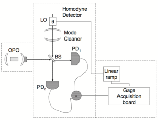
The source is a below threshold fully degenerate OPO based on a type–I LiNbO₃:MgO crystal and pumped at 532 nm APB2001 . The quantum homodyne detector, whose reliability has been proved in different experiments solimeno ; CovMat , shows an overall quantum efficiency of $\eta=0.88\pm 0.02$. To avoid any influence on the statistics of the data, the electronic noise floor is kept $\approx 15$ dB below the shot noise. Mode matching at the BS has been accomplished by spatially filtering the local oscillator (LO) beam by a mode cleaner cavity whose geometrical properties match the OPO’s ones. The relative phase between the LO and the beam exiting the OPO is scanned by a piezo mounted mirror to which a linear voltage ramp is applied; the ramp is adjusted so to have a 2$\pi$ phase span in the acquisition time. The 2$\pi$ variation necessary for a full state reconstruction is selected in the central region of the piezo range so to optimize the linear response of the piezo stack.

Figure 2: Raw homodyne data for the vacuum state (top) and for the OPO output close to threshold (bottom).

Data sampling is moved away from the laser carrier frequency by mixing the homodyne current with a sinusoidal signal of frequency $\Omega=3$ MHz. The resulting current is low–pass filtered with a bandwidth $B=1$ MHz, and eventually sampled by a digital acquisition PC based module (Gage 14100) able to acquire up to 1M–points per run with 14 bits resolution. For each state, 1 048 308 quadratures values were measured.

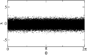
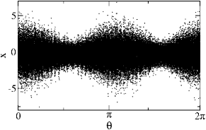
Measured quadrature values normalized with respect to vacuum fluctuations are shown in Fig. 2. To facilitate our analysis the data were grouped into $31$ phase bins prior to reconstruction. The purpose of the experiment was to perform Gaussian tomography and compare the results with that of the standard homodyne tomography objectivetomo where no assumption about the Gaussianity of the measured state were made. The comparison of the reconstructed states may be seen as a test of Gaussian behavior. Such an approach is superior to a test based on evaluating certain quadrature moments due to the fact that all the relevant moments are encoded in the reconstructed state.

The Gaussian analysis starts with evaluating quantities $y_{h}=\sum_{k}x_{h,j}^{2}$ for each phase bin $\theta_{h}$, $h=1,31$. These are used to construct operator $R$ appearing in the extremal equation for covariance matrix Eq. (13). The following covariance matrices were found for measured vacuum (V) and OPO (O) data:

$$G_{\text{V}}=\left(\begin{array}[]{cc}0.50&0.00\\ 0.00&0.50\end{array}\right),\,\,G_{\text{O}}=\left(\begin{array}[]{cc}2.38&-0.53\\ -0.53&0.55\end{array}\right).$$ (36)

Matrix $G_{\text{O}}$ indicates that the reconstructed Wigner function of the OPO state is slightly rotated with respect to the $x$-$p$ axes, which are defined by the the phase of the local oscillator. The squeezed nature of the input signal is revealed by diagonalizing matrix $G_{\text{O}}$. With that variances of $0.40$ and $2.53$ are found for the squeezed and anti-squeezed quadratures, respectively. Notice that the reconstructed state is not a minimum-uncertainty state, $\text{Det}\,G_{\text{O}}=1.02\gg 1/4$ and so the reconstructed covariance matrix is located well inside the set of physical covariance matrices, $G_{\text{O}}>\Omega$. To summarize the Gaussian analysis, a squeezed Gaussian state is inferred from experimental data whose anti-squeezed quadrature has been contaminated by some classical excess noise. Now it is interesting to compare the result of Gaussian analysis with that of the generic quantum tomography applied to the same data set. In this case, no assumption is made about the Gaussian character of the measured signal and the reconstruction is done on an $N$-dimensional truncated Fock space using the maximum-likelihood technique objectivetomo . Data have been grouped into $31$ phase bins. In addition, detections within each phase bin have been divided into $31$ quadrature bins. The set of quadrature projectors corresponding to the $31\times 31=961$ pairs of phase and quadrature values comprises a POVM describing the tomography scheme. Prior to reconstruction, the dimension $N$ of the reconstruction space must be chosen. Notice that this parameter has no analogy in the Gaussian analysis above.

Figure 3: Hilbert-Schmidt distances of state reconstructions done in $N$-dimensional Fock spaces with respect to the reference state reconstructed in dimension $N=30$.

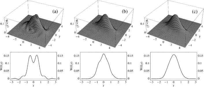
In order to see the effects of the truncation on the reconstructed state, the procedure has been repeated for different values of $N$. The convergence of the generic reconstruction with growing reconstruction space is shown in Fig. 3, where the Hilbert-Schmidt distance $d_{\text{HS}}=\text{Tr}\{(\rho_{N}-\rho_{30})^{2}\}$ between a reconstruction from a truncated space and a reference reconstruction from a large space is plotted as a function of $N$. This figure indicates that from $N=10$ on the reconstructed state does not change significantly when the reconstruction space is enlarged. This conclusion, however, turns out to be incorrect when one is interested in qualitative, rather than quantitative properties of the reconstructed state. For instance, the shape of the reconstructed Wigner function may help to classify the signal as being Gaussian or non-Gaussian. Similarly, the presence of negative values of $W$ may be taken as a sign of non-classical behavior. In turn, making qualitative statements from quantitative results of tomography may be delicate and challenging. This is illustrated in Fig. 4, where we report the Wigner function and the corresponding y-cut for different values of the truncation dimension for the reconstruction in the Fock space. Notice that what may seem as a sign of non-classical interference in Fig. 4(a) is actually an artifact due to small value of the reconstruction dimension. Remarkably, this happens even though the inspection of the elements of $\rho_{15}$ and $\rho_{25}$ in the Fock basis shows negligible differences (see also Fig. 3), since these tiny differences get amplified when switching to Wigner representation. Also plots in Fig. 4(b) distinctly shows non-Gaussian shapes and the artifacts are present until dimension of $N\approx 25$ is reached. In this region the generic reconstruction starts to be consistent with the Gaussian results yielding very similar values of quadrature variances. More than $600$ free parameters must be introduced in the standard tomography to achieve the quality of the simple Gaussian fit of OPO data!

There remains a question whether the deviations from Gaussian character that may be observed in the generic reconstruction even for large dimensions $N$ are real features of the measured state or not. This possibility may be confirmed or discarded by analyzing the scores (likelihoods) achieved by the Gaussian and generic reconstructions respectively. Here, a direct comparison is not possible due to different natures of involved data. Instead, one may determine how much the quality of the fit degrades by replacing vacuum data with the more noisy OPO signal. For Gaussian analysis we find that the log-likelihood of the OPO reconstruction is smaller by a factor $3.66$ compared to the vacuum reconstruction. Standard tomography yields a smaller factor of $3.16$, which indicates that a better fit of the OPO signal generated near the threshold is obtained by abandoning the Gaussian hypothesis.

Figure 4: Wigner functions (upper row) and cuts along the $y$ axis (bottom row) of the OPO state reconstructed in Fock spaces of dimensions $N=8$ (a), $N=15$ (b), and $N=25$ (c) respectively.

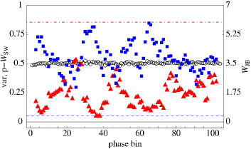
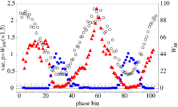
In order to test the null hypothesis for our samples (i.e., data normally distributed) we grouped homodyne data into phase bins made of $10\,000$ outcomes each and applied “normality tests” to both the samples of Figs. 2. In particular, we have used the Jarque-Bera (JB) JB:80 and the Shapiro-Wilk (SW) normality tests SW:65 . The JB test is based on both the skewness $S$ and the kurtosis (excess) $K$ of the sample, i.e

$$S=\frac{\mu_{3}}{(\mu_{2})^{3/2}}\,,\quad K=\frac{\mu_{4}}{(\mu_{2})^{2}}-3\,,$$ (37)

where $\mu_{k}\equiv\frac{1}{N}\sum_{h=1}^{N}(x_{h}-\overline{x})^{k}$ is the $k$-th central moment, $N$ is the number of data and $\overline{x}$ their mean. The JB statistics is then defined as:

$$W_{\rm JB}=\frac{N}{6}\left(S^{2}+\frac{1}{4}K^{2}\right).$$ (38)

Since $W_{\rm JB}$ has an asymptotic $\chi^{2}$ distribution with two degrees of freedom JB:80 , one can use it to test the null hypothesis of normality. In particular, by choosing a significance level $0.05$, one rejects the null hypothesis if $W_{\rm JB}>5.99$. The test statistics $W_{\rm SW}$ of the SW test reads as follows:

$$W_{\rm SW}=\frac{\left(\sum_{h=1}^{N}a_{h}x_{(h)}\right)^{2}}{\sum_{h=1}^{N}(x_{h}-\overline{x})^{2}},$$ (39)

where $x_{(h)}$ are the ordered sample values ($x_{(h)}$ is the $h$-th smallest value) and $a_{h}$ are constants generated from the means, variances and covariances of the order statistics of a sample of size $N$ from a normal distribution SW:65 . In this case one rejects the null hypothesis of normality within a significance interval of $0.05$, if $p$-$W_{\rm SW}\leq 0.05$, where the $p$-$W_{\rm SW}$ is the $p$-value of $W_{\rm SW}$, i.e. the probability of obtaining a result at least as extreme as the one that was actually observed, given that the Gaussian hypothesis is true. The two test statistics are shown in Fig. 5, where we plotted the variance, $W_{\rm JB}$ and $p$-$W_{\rm SW}$ associated with the data of Figs. 2. As one can see, the vacuum data are normally distributed, whereas those coming from the OPO close to threshold show clear deviations from the Gaussian behavior (see also solimeno ), thus justifying the rejection of Gaussian hypothesis.

Figure 5: (Color online) Variance (circles), $W_{\rm JB}$ (triangles) and the $p$-value of $W_{\rm SW}$ ($p$-$W_{\rm SW}$, squares) associated with the homodyne data of Figs. 2. Top: vacuum data. Bottom: OPO close to threshold data (here $p$-$W_{\rm SW}$ has been magnified by a factor $\times 1.5$). The dashed line is the threshold value $0.05$ for $p$-$W_{\rm SW}$ ($\times 1.5$ in the bottom plot); the dot-dashed line is the threshold value $5.99$ for $W_{\rm JB}$. If $W_{\rm JB}\geq 5.99$ and/or $p$-$W_{\rm SW}\leq 0.05$, then the null hypothesis (Gaussian states) is rejected. See the text for details. Results indicate that vacuum data (top) are consistent with the Gaussian hypothesis whereas for data coming from the OPO close to threshold the Gaussian hypothesis should be rejected.

VI Conclusions

In this paper, upon exploiting the formal analogies between the description of Gaussian states and that of finite-dimensional quantum states, we have proposed and demonstrated a simple and efficient method for the reconstruction of Gaussian states. The method have been tested numerically and applied to the reconstruction of the quantum state of the signal generated by an optical parametric oscillator. As a matter of fact, under the Gaussian hypothesis there is a drastic reduction in the number of parameters needed to characterize a quantum state, and this leads to a robust reconstruction technique. Indeed, our results indicate that on Gaussian and near Gaussian states the proposed method provide a more stable and reliable reconstructions than standard tomography techniques. We have also shown that putting together results coming from the Gaussian method with those coming from standard tomography, we obtain a reliable tool to detect the non-Gaussian character of optical signals. We conclude that the present method provides a reliable and robust tool for the characterization of quantum states which may be of interest for a rather broad community working in continuous-variable quantum information processing and quantum state reconstruction.