The Complete Initial Mass Function Down to the Sub-Solar Regime in the Large Magellanic Cloud with Hubble Space Telescope ACS Observations

Abstract

In this photometric study of the stellar association LH 95 in the Large Magellanic Cloud (LMC) we focus on the pre-main Sequence (PMS) population in order to construct, for the first time, the sub-solar initial mass function (IMF) in the LMC. The basis for this investigation consists of the deepest photometry ever performed in the LMC with the Advanced Camera for Surveys (ACS) on-board the Hubble Space Telescope (HST). We improve our catalog of point sources obtained with ACS (Paper I). We carry out a Monte Carlo technique to subtract the contribution of the general field of LMC. We isolate the central region in the observed area of the association, as the part characterized by the highest concentration of PMS stars. We analyze the reddening distribution of the system in order to obtain the mean value of extinction and we study the mass function of its field-subtracted population. For this purpose, we introduce a new set of evolutionary models, derived from the calculations on the evolution of PMS stars by Siess and collaborators. We use these models with our observations of LH 95 to derive the IMF of the system. This mass function is reliably constructed for stars with masses down to $\simeq 0.43$ M_⊙, the lowest mass ever observed within reasonable completeness in the Magellanic Clouds. Consequently, its construction offers an outstanding improvement in our understanding of the low-mass star formation in the LMC. The system IMF of LH 95 shows a definite change in its slope for masses $M\lesssim 1$ M_⊙, where it becomes more shallow. In general, the shape of this IMF agrees very well with a multiple power-law, as the typical Galactic IMF, down to the sub-solar regime. The change in the slope (“the knee”) of our IMF at $\sim 1$ M_⊙ also agrees with the average Galactic IMF. As far as the slope of this system IMF is concerned, it is found to be somewhat more shallow than the corresponding “classical” Galactic IMF in the sub-solar regime, probably due to unresolved binarity, while for stars with $M\ \raise-2.0pt\hbox{\hbox to0.0pt{\hbox{$\sim$}\hss}\raise 5.0pt\hbox{$>$}\ }1M\mbox{${}_{\normalsize\odot}$}$ it becomes slightly steeper. We do not find significant differences in the shape of the overall IMF of LH 95 from that of each of the three individual sub-clusters of the association. This clearly suggests that the IMF of LH 95 is not subject to local variability.

1. Introduction

The Magellanic Clouds, the closest undisrupted dwarf galaxies to our own galaxy, host numerous young stellar associations. The study of the low-mass populations of these systems provide important improvements in understanding extragalactic star formation. The investigation of the star formation processes, and the Initial Mass Function (IMF), together with the time dependency of the formation events, are key points in the characterization of stellar populations in any kind of concentrations, from small clusters to entire galaxies.

Regarding the IMF, several studies have been carried out in the past for the Galaxy (e.g. Salpeter, 1955; Scalo, 1986; Kroupa, 2001; Chabrier, 2003), describing the initial numbers of massive stars ($M\gtrsim 8$ M_⊙), stars of intermediate mass ($1$ M${}_{\odot}\lesssim M\lesssim 8$ M_⊙), low-mass stars ($0.08$ M${}_{\odot}\lesssim M\lesssim 1$ M_⊙) and brown dwarfs ($M\lesssim 0.08$ M_⊙). The findings of such investigations support the hypothesis of the universality of the IMF, in the sense that the average IMF measured in a diversity of galactic systems does not show noticeable variations (Kroupa, 2002). This statement turns out to be rather certain for the intermediate- and high-mass stars, while for low-mass stars there could be a dependence of the IMF slope on metallicity, in the sense that metal-rich environments tend to produce more low-mass stars than metal-poor systems (Piotto & Zoccali, 1999; Reylé & Robin, 2001), although several IMF measurements are needed to confirm such a systematic effect. In low-mass studies there are several uncertainties present. For example the study of the IMF in metal-poor galactic globular clusters (Piotto & Zoccali, 1999) is significantly limited by the corrections for dynamical evolution effects. Specifically, phenomena such as mass segregation and unknown binarity fraction change dramatically the presently measured mass distribution with respect to the one at the time of the formation of these systems (Marks et al., 2008).

Under these circumstances, ideal environments for the search of a metallicity dependence of the IMF are the Magellanic Clouds. Their stellar populations are characterized by metallicities of $[Fe/H]\simeq 2.5$ to $5$ times lower than in the disk of the Milky Way (Luck et al., 1998), but have a similar star formation rate (SFR) (Westerlund, 1997). Furthermore, the low metal abundances of the Magellanic Clouds suggest that their environments $-$ as well as in other galaxies of the Local Group $-$ are closer to the ones at the early ages of the universe, when the peak of star formation occurred ($z\simeq 1.5$, Pei et al., 1999). Moreover, the lower dust-to-gas ratio in the Magellanic Clouds (Koornneef, 1982; Bouchet et al., 1985), in comparison with the Milky Way, assures a lower extinction, reducing the bias introduced by differential reddening, a well known limitation in the study of young stellar populations.

Table 1Sample from the photometric catalog of all stars found in the region of LH 95 with HST/ACS imaging

	R.A.	DECL.	$F555W$	$\sigma_{\rm 555}$	$F814W$	$\sigma_{\rm 814}$
#	(J2000.0)	(J2000.0)	(mag)	(mag)	(mag)	(mag)
1	05 37 06.04	$-$66 21 37.15	14.839	0.001	15.066	0.001
2	05 37 19.26	$-$66 21 07.88	15.956	0.001	15.001	0.001
3	05 36 59.26	$-$66 21 20.66	15.406	0.001	15.570	0.001
4	05 37 15.12	$-$66 21 44.39	15.503	0.001	15.494	0.001
5	05 37 05.62	$-$66 21 35.39	15.372	0.001	15.473	0.001
6	05 36 49.60	$-$66 23 26.16	16.930	0.003	14.873	0.001
7	05 37 05.53	$-$66 21 59.65	15.632	0.001	15.740	0.001
8	05 37 04.53	$-$66 22 01.02	15.670	0.001	15.783	0.002
9	05 37 14.29	$-$66 22 52.00	15.951	0.001	15.990	0.001
10	05 36 56.68	$-$66 21 10.40	16.828	0.001	15.102	0.001
11	05 36 53.49	$-$66 21 55.55	17.183	0.002	15.595	0.001
12	05 36 59.67	$-$66 22 02.10	16.813	0.001	14.982	0.001
13	05 37 01.86	$-$66 22 35.65	16.752	0.002	15.663	0.001
14	05 36 57.29	$-$66 21 49.03	16.267	0.001	16.440	0.001
15	05 36 53.06	$-$66 22 11.28	16.610	0.001	16.736	0.002
$\cdots$	$\cdots$	$\cdots$	$\cdots$	$\cdots$	$\cdots$	$\cdots$

Note. — Magnitudes are given in the Vega system. Units of right ascension are hours, minutes, and seconds, and units of declination are degrees, arcminutes, and arcseconds. The spatial resolution of the ACS/WFC is 0.05^′′ .

Most of the star formation occurs in dense cores of Giant Molecular Clouds, where one or more large stellar concentrations, known as OB associations (Ambartsumian, 1947), are formed. However, most of the star formation studies in the Milky Way are carried out in smaller fields, like the young Taurus, Lupus and Chamaeleon star-forming regions. Although it has been shown that galactic OB associations host populations of faint, low-mass PMS stars (Preibisch et al., 2002; Sherry et al., 2004; Briceño et al., 2007) their analysis is strongly limited by the contamination of background and foreground evolved populations, requiring detailed measurements of proper motions, time-consuming spectroscopy and multi-epoch photometry to define their membership. On the other hand, the study of OB associations in the LMC is less subject to contamination by field populations, due to the limited distance spread (Caldwell & Coulson, 1986; Cole, 1998). However, in order to identify the faint red PMS stellar component of LMC associations, photometry with instruments of high sensitivity and angular resolution is required, due to the larger distance from us.

Recent findings from the Hubble Space Telescope (HST) confirm the presence of PMS stars in OB associations of the Magellanic Clouds. Gouliermis et al. (2006a) studied this case in the LMC association LH 52, using WFPC2 observations in the $V$- and $I$-equivalent bands, and they discovered a population of objects in the color-magnitude diagram (CMD) consistent with T-Tauri stars. Subsequently, the Advanced Camera for Surveys (ACS) has been used to perform similar studies in other associations of the Magellanic Clouds, such as NGC 346 (Nota et al., 2006; Gouliermis et al., 2006b; Hennekemper et al., 2008; Sabbi et al., 2008) and NGC 602 (Schmalzl et al., 2008) in the SMC. However, these studies could not characterize the sub-solar mass function, because of the insufficient detection of such stars.

In the first part of our study ACS observations enabled us to discover a rich population of PMS stars in the star-forming region LH 95 in the LMC (Gouliermis et al., 2007, from hereafter Paper I). In this paper we focus on the IMF of these stars, which is reliable for masses down to about $0.3$ M_⊙, considering that our photometry allowed to perform precise completeness corrections for stars with masses down to this limit. In § 2 we describe our photometry and the completeness of our data. In § 3 we apply the decontamination of the observed stellar sample in the area of the association LH 95 from the contribution of the general LMC field for the identification of the stellar members of the system. We also investigate the spatial distribution of the identified pre-main sequence population, in order to define the limits of the main body of the system, and we apply extinction measurements. In § 4 we present our calculations for new PMS evolutionary models in the observational plane. We make use of these models in combination with our photometry for the construction of the system IMF of LH 95 in § 5. We discuss our findings in § 6 and final conclusions are given in § 7.

Figure 1.— $F555W-F814W$, $F814W$ Color-Magnitude Diagram of the entire LH 95 region, according to the updated photometric catalog, which includes about 900 stars more, recovered by visual inspection of the sources rejected in the photometric study of Paper I. It is worth noting that, besides a dense main-sequence population, this CMD is characterized by a remarkable number of PMS stars at faint magnitudes and red colors, as indicated in Paper I.

2. Photometry

In this study we analyze the photometry presented in Paper I, derived from deep observations with the Wide-Field Channel (WFC) of ACS on-board HST within the GO Program 10566 (PI: D. Gouliermis). Two pointings were observed, one centered on the association LH 95 itself, which we refer to as the “system”, and another one about 2^′ to the west on an empty area, typical of the local LMC field. We refer to the latter as the “field”. For each pointing observations in two photometric bands were available: F555W and F814W, roughly equivalent to the Johnson V and Cousins I bands respectively. The observations and their photometry are described in detail in Paper I. We found about 16,000 stars in the system, about 2,600 of which lie in the PMS region of the CMD, and about 17,000 in the field.

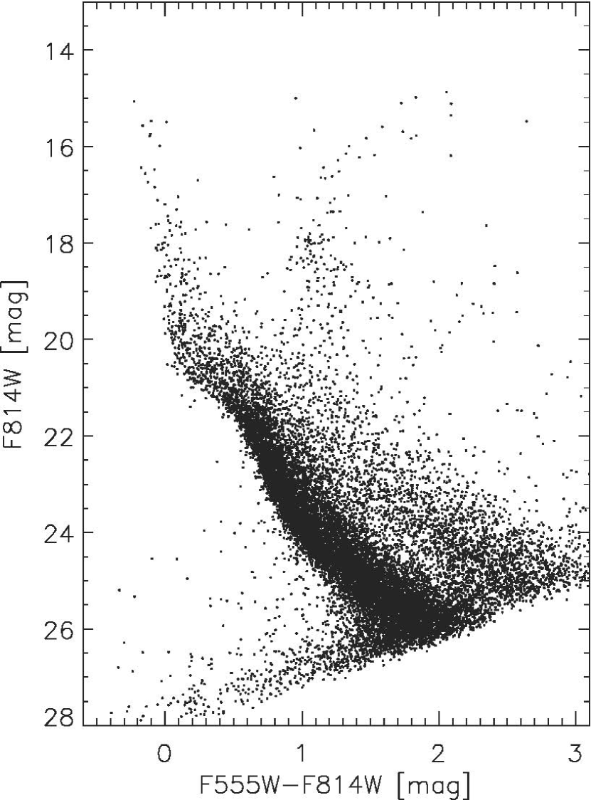
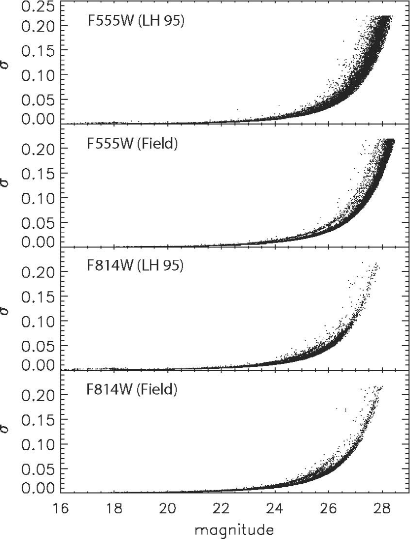
In the present work we enhance the photometric catalog of stars derived in Paper I by searching for eventually missing objects, especially in the low-mass PMS regime. Photometry was obtained using the ACS module of the package DOLPHOT (Ver. 1.0). The selection of stars in our original photometry was based on the quality parameters estimated for each detected source by the package. However, objects which are actual stars may have been rejected as spurious detections in crowded regions, especially in the presence of a non-uniform background due to nebular emission, as well as in the neighborhood of very bright sources. Therefore, we considered the catalog with all the rejected sources and we performed a visual inspection of each of them on the original ACS FITS images constructed with Multidrizzle. With this process we recovered about 900 additional stars. The updated photometric catalog of the association LH 95 includes in total 17,245 stars. A sample of this catalog is shown in Table 1. The corresponding CMD is shown in Fig. 1. Typical uncertainties of our photometry as a function of the magnitude for both filters are given in Figure 2 (left), for both the “system” and the “field” ACS pointings.

Figure 2.— Left panel: Distribution of the photometric errors, for both the F555W and F814W band for the LH95 system and the LMC field. Right panel: Completeness of our photometry in the entire observed areas of both the system (top) and the field (middle), as well as for the central region of the association LH 95 (see § 3.2).

2.1. Completeness

The completeness of the data is evaluated by artificial star experiments with the use of lists of almost 400,000 artificial stars created with the utility acsfakelist of DOLPHOT for each of the observed areas of the system and the field. This utility enables to add stars of given magnitudes to all the frames simultaneously, searching for a detection in none, one, or both photometric bands. In this way it is possible to derive automatically a 2-dimensional completeness function for both color ($F555W-F814W$) and magnitude $F555W$ or $F814W$. Considering that at any given faint magnitude in one band the color term covers a range of up to $2$ magnitudes, as shown in the CMD of Figure 1, allowing the magnitude in the other band and therefore the completeness to vary significantly, this two-dimensional approach is necessary for an accurate treatment of the completeness of our data. Therefore, we define with our artificial star technique the 2D completeness as a function of ($F555W-F814W$) and $F814W$, by computing the ratio of the detected sources over the total added stars in a grid of equally spaced bins $0.25$ magnitudes wide in ($F555W-F814W$) and and $0.5$ magnitudes in $F814W$.

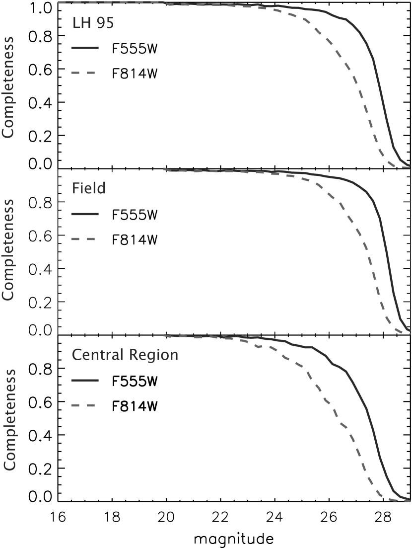
Such completeness maps have been constructed for both the system and the field, enabling, via interpolation, an accurate determination of the actual completeness at any given point of the CMD. The right panel of Figure 2 shows the completeness function in both bands for both the system and the field (top and middle respectively). The completeness is found to vary with location, and therefore different regions in the observed field-of-view are characterized by different completeness functions according to their crowding. In the bottom panel of the figure we show the completeness as a function of magnitude for the central region of the association, as it is defined in § 3.2. It is remarkably lower than that in the entire field-of-view, due to higher crowding of faint stars and over-density of the bright ones.

To avoid further contamination by spurious objects in our catalog, which could have been included through additional stars, we trimmed the data set used in this work excluding sources with $V>28.5$ mag or $I>28$ mag. At these magnitude limits stars are faint enough to be well below any reasonable completeness limit. The completeness in the “system” CMD at V=$28.5$ mag and I=$28$ mag is less than 1%. Consequently, their removal does not affect the quality and completeness of our data.

3. The Pre-Main Sequence Population of LH 95

3.1. Field subtraction

The observed stellar population in the area of the association LH 95 is naturally contaminated by the general field population of LMC. Therefore, in order to study the stellar members of the association alone, and in particular its PMS stars, the field contamination should be removed. In our case, having at our disposal photometry in only two bands, the possibility to distinguish if a given star is a true member or not is limited, but a statistical approach can provide accurate results.

We use a Monte Carlo technique, which considers that a star belongs to the cluster or the field with a probability, which depends on the local density in the same part of each CMD (of system and field). In order to maximize the statistical accuracy of the result, two iterations are applied. First, the field subtraction is applied to the entire observed field-of-view centered on the system, enabling to study the spatial distribution of the LH 95 stars and to isolate the boundaries of the association. After that, the study is limited on this subregion of the frame, and another field subtraction is carried out on the central region providing an accurate estimate of the membership of the sources included.

Specifically, for the first iteration we consider each star in the catalog of the system and we select an elliptical region in the CMD of the system centered on the position of this star, and the same region in the CMD of the field. Each such region is being chosen with semi-axes $\Delta I=0.5$ mag and $\Delta(V-I)=0.17$ mag. This particular size has been chosen as to be wide enough to include a considerable number of stars, and still small enough to achieve a considerably high resolution in the resulting CMD. We compute the probability of each star in the area of the system to belong to the field as:

$$P=A\cdot\frac{N_{\rm fld}}{N_{\rm sys}}\cdot\frac{C_{\rm sys}}{C_{\rm fld}}$$ (1)

where $N_{\rm sys}$ and $N_{\rm fld}$ are the numbers of stars included in the elliptical region of the CMD of the system and the field respectively. $C_{\rm sys}$ and $C_{\rm fld}$ are the completeness factors, for system and field, measured for exact position of the considered star in the CMD, as explained in § 2.1. $A$ is a normalization factor which takes into account differences in the field stellar density between the two regions. From repeating measurements in different parts of the area of the field and that of the system we found that on average the field includes systematically $\sim 1.3$ times more main sequence stars than LH 95. Therefore, considering that both areas cover equal surfaces, we set $A=0.77$. According to Eq. 1, when $P\geq 1$ the star is considered to be a field star and it is removed; $P=0$ means that there are no field stars in the field CMD in the elliptical neighborhood of the star and therefore it is considered a member of the association. When $0<P<1$ the star is randomly kept or rejected as a member star with a probability equal to $P$.

Figure 3.— $F555W-F814W$, $F814W$ Color-Magnitude Diagram (CMD) of the entire observed area around LH 95. The stars which are identified as members of the system alone and not of the field of the LMC based on the first field-subtraction iteration (see § 3.1) are plotted with thick symbols. The dashed line sets the limits of the loci in the CMD of the PMS alone. The spatial distribution of these stars has revealed the existence of young stellar sub-groups within the association (Paper I; see also § 3.2).

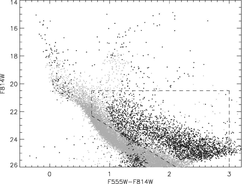
The result of the first field-subtraction iteration, applied to the entire LH 95 field of view is shown in Fig. 3, where stars flagged to belong to the association are plotted by black dots. As shown in Paper 1, it is evident that the PMS population belongs entirely to LH 95, while all lower main sequence stars turn out to belong to the LMC field. The upper main sequence (UMS) shows an overabundance of stars in the area of the system, demonstrating the presence of the corresponding population in the association itself.

3.2. Topography of the PMS Stars

In this section we study the spatial distribution of the PMS stars in the area of LH 95, as an indication of the places where star formation occurs. For this purpose, we construct surface density maps of the whole area by counting the stars identified as system members after applying the Monte Carlo removal of the field contamination as described in § 3.1. Since we are interested in the PMS cluster properties, we considered only the PMS population, as selected in the region of the CMD shown in Figure 3.

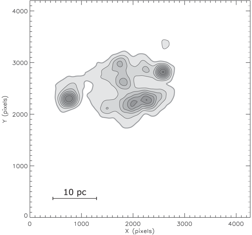
The star counts are performed by dividing the whole ACS field-of-view into a grid of $50\times 50$ elements, each corresponding to a size of $\sim 85$ pixels ($\simeq 1$pc), and by counting the (field-subtracted) PMS stars in each of them. The selection of the specific grid-element size, which corresponds to the “resolving efficiency” of the detection of stellar concentrations, was chosen, after several experiments, as the most appropriate for revealing the smallest concentrations with a physical meaning.

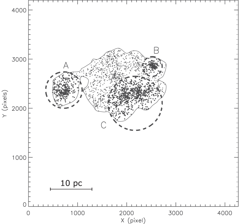
In order to remove from this map eventual noise, we applied a smoothing on the density map with a kernel of size $\sim 2.5$pc $\simeq 200$ pixels. The majority of the PMS stars is found to be located within a compact region $\sim 1\hbox{${}^{\prime}$}\times 2\hbox{${}^{\prime}$}$, with a density well above the threshold of $3\sigma$, where $\sigma$ is the standard deviation of the background surface density. The derived two-dimensional density map is shown in Figure 4 (left), where the $3\sigma$ density limit, corresponding to the first (lower) isopleth, is chosen to define the statistically significant concentration of the PMS population of the association LH 95.

Figure 4.— Left panel: Isodensity contour map of the area of the system constructed from star counts of the PMS stars alone. Isopleths are drawn in steps of 1$\sigma$, where $\sigma$ corresponds to the standard deviation of the background density, starting from the 3$\sigma$ level. This level defines the limits chosen for the selection of the stars used for the construction of the CMD of the central part of the area of the system shown in Figure 5 (left and right panels). This map demonstrates that, as we found in Paper 1, PMS stars are concentrated in few compact subgroups within the association. These density peaks in the PMS stars coincide with those of the Upper Main Sequence (UMS) stars (Paper I), suggesting that these subgroups contain fully populated IMFs. Units are in pixels on the ACS drizzled frame. Right panel: Positions of the three most prominent concentrations (subclusters) of PMS stars, which appear as the densest substructures of the main part of the association LH 95.

Table 2Characteristics of the Central Region (LH 95) and its three subclusters

	RA	DEC	Size	$r_{\rm h}$	$M_{\rm tot}$	$\varrho$	$t_{\rm d}$	$t_{\rm cr}$	$t_{\rm relax}$
	(J2000.0)	(J2000.0)	(pc)	(pc)	(103 M⊙)	(M⊙ pc-3)	(100 Myr)	(Myr)	(Myr)
LH 95	5 37 06.50	$-$66 22 03.50	33.5	6.5	2.37	0.47	0.9	6.4	433.0
A	5 37 15.25	$-$66 21 40.87	8.7	1.7	0.33	1.28	2.4	2.2	26.9
B	5 36 59.78	$-$66 21 36.88	4.7	0.8	0.19	2.70	5.1	0.9	6.7
C	5 37 03.96	$-$66 22 09.73	12.9	3.0	0.98	1.11	2.1	3.1	95.5

From here on, we refer to the region confined by the $3\sigma$ density isopleth of Figure 4 as the central region of LH 95, and we focus our subsequent analysis on the stellar population included within the boundaries of this region, as the most representative of LH 95. In Figure 4 (left) can be seen that within the central region there are smaller substructures characterized by a higher projected density of PMS stars. We select the three most prominent ones, isolating circular areas within the central region as shown in Figure 4 (right). We refer to these substructures as subcluster A, B and C respectively. The positions and sizes of the selected circular regions around the subclusters, shown in Figure 4 (right), are given in Table 2 with those for the whole central region. We measure the total mass, $M_{\rm tot}$, included in each stellar concentration, assuming that all systems follow a mass function similar to the standard Galactic field IMF (Kroupa, 2002), and extrapolating their stellar content down to 0.08 M_⊙. We then estimate the stellar density, $\varrho$, and the disruption time, $t_{\rm d}$, of each cluster following the method by Gouliermis et al. (2002, their section 6). The latter is given as (Spitzer, 1958):

$$t_{\rm d}=1.9\times 10^{8}\varrho\bigg{(}\frac{{\rm M}_{\odot}}{{\rm pc}^{3}}\bigg{)}~{}~{}{\rm years}~{}.$$ (2)

Moreover, the dynamical status of a stellar system is defined by two additional time-scales, the crossing and the two-body relaxation time (Kroupa, 2008), which are given as:

$$t_{\rm cr}\equiv\frac{2r_{\rm h}}{\sigma}~{}~{}~{}{\rm and}~{}~{}~{}t_{\rm relax}=0.1\frac{N}{\ln{N}}t_{\rm cr}$$ (3)

respectively. The three-dimensional velocity dispersion of the stars in the cluster, $\sigma$, is given as

$$\sigma=\displaystyle{\sqrt{\frac{{\rm G}M_{\rm tot}}{\epsilon r_{\rm h}}}~{}~{},}$$ (4)

where $\epsilon$ is the star formation efficiency (SFE) and $r_{\rm h}$ the half-mass radius of the cluster. In order to make a rough estimation of the aforementioned time-scales for the subclusters and the whole central region of LH 95, we apply the formulas of Eq. 3.

The SFE in several nearby Galactic gas-embedded clusters has been found to range typically from 10% to 30% (Lada & Lada, 2003) or 20% to 40% (Kroupa, 2008), value which increases with time while the gas is removed. However, the average age of the system is 4 Myr (see §5), slightly greater than the typical time necessary to remove most of the gas (Lada & Lada, 2003). Therefore, and taking into account the very low optical extinction (see §3.2), LH 95 should be considered as an emerging cluster, meaning that it should be at the process of separation from the parental cloud. Furthermore, according to Wilking & Lada (1983), a high SFE is required for a bound young cluster to emerge from its parental cloud. As a consequence, we consider a value of $\epsilon\simeq 0.4$ as more adequate for our system. We derive, thus, values of $\sigma$ of the order of 2 km s^-1 for our objects and we provide the additional estimated structural parameters for each system also in Table 2. We find that the crossing time for the whole region is greater than the age of the system, and this is quite consistent with the observed sub-clustering of the system.

From a comparison between the characteristics of the subclusters and the central region, as they are given in Table 2, one can see that there is a significant fraction of mass outside the immediate regions of the subclusters. This can also be seen in the maps of Figure 4, where a prominent population of PMS stars is easily distinguished away from the subclusters, spread in the area among them within the central region. We estimate that the fraction of distributed stellar mass over the total corresponds to $\sim$ 40%, with the remaining 60% being clustered. This fraction of distributed PMS stars in LH 95 is consistent with statistical analyses of several Galactic nearby star-forming regions that predict  $\sim$$<$  60% (see review by Allen et al., 2007). However, it is not clear if this distributed population is the result of the star formation or a merging process. Detailed simulations do predict that subclusters may merge to form a larger one (e.g. Fellhauer et al., 2006), but our data do not allow us to verify if this takes place in LH 95. In any case, the stellar density and disruption time of all considered systems, including the whole central region, show that all are rather compact and none of them is under disruption. Subclusters A and B, located at the east and west of the central region, are particularly compact and roughly spherical shaped, while subcluster C, close to the southern limit of the central region, presents a more elongated and extended distribution of PMS stars. This subcluster corresponds to the visibly prominent main part of the association (see Figure 1 in Paper I).

Figure 5.— Left: CMD of all stars observed in the central part of the area of the system. This part was selected as the most representative of the association based on star counts (§ 3.2; Figure 4). Middle: CMD of the corresponding part of the area of the field, which was used for the decontamination of the CMD of the system from the contribution of the field stellar population. Right: CMD of central area of the system after the field subtraction was applied with the use of an advanced Monte Carlo method (§ 3.1). This CMD highlights the UMS and PMS stars as the prominent stellar populations of the association LH 95, demonstrating its youthfulness.

3.3. LH 95 Central region

For the detailed study of the PMS population in LH 95, while minimizing the contamination by other stars, we focus on the central region of the system. Specifically, we consider the entire population included in the central region and we apply, for a second time, the Monte Carlo technique for field subtraction, taking into account the ratio between the surface of the observed LMC field and that of the central region.

It should be noted that this second application of the field subtraction technique to the central region is not equivalent of simply isolating the stars, which are found to be located within the boundaries of the region after the first iteration of the Monte Carlo subtraction.

Naturally, the central region has a higher density of system stars (specifically PMS stars), and therefore a lower relative contamination by field stars. Consequently, the actual fraction of stars which are marked to be field stars is lower, reducing the probability of (statistically probable) wrong membership assignments. The number of field stars included in the elliptical region of the CMD $N_{\rm fld}$ is computed based on the photometry in the entire field and scaled according to the area occupied by the LH 95 central region, which we found to be $\sim~{}12.6\%$ of the total ACS field-of-view.

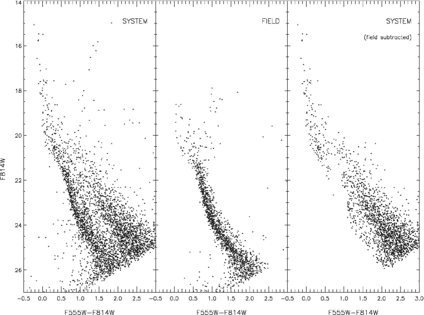
The result is shown in Figure 5, where we plot the CMDs of the whole population included within the boundaries of the central region (left panel), the one of the whole area of the field, sampled randomly and down-scaled according to the area coverage of the central region (central panel), and the corresponding CMD of the central region after the field contribution has been removed (right panel). From this figure it is evident that the observed stellar population of the low main sequence (LMS) can be entirely considered as field population. On the other hand the association has a prominent upper main sequence (UMS) component, and all pre-main sequence stars, easily distinguished by redder colors, are solely present in LH 95 alone. Furthermore, the second application of our field subtraction technique, limited to the central region, allows us to reduce considerably the contamination by objects not located in the PMS and UMS parts of the CMD, which are still present as residuals from the first application of the method on the entire field-of-view (Figure 3).

In the CMDs of Figure 5 can be noted that the field population has a tighter sequence than the PMS population, which may indicate an age-spread among the PMS stars of LH 95 (see also Figure 9). Indeed, the locations of low-mass PMS stars in the CMD of young stellar systems of our Galaxy often show a widening, which may be evidence for an age-spread in the system (e.g. Palla & Stahler, 2000). However, several characteristics of these PMS stars (being T Tauri stars), such as variability and circumstellar extinction, can cause considerable deviations of their positions in the CMD (Sherry et al., 2004), which may be misinterpreted as an age-spread. As a consequence, detailed simulations of the characteristics of PMS stars are required to quantify the effect of these characteristics on their positions in the CMD and to conclude on any true age-spread (Hennekemper et al., 2008) with the use of population-synthesis techniques.

In the following sections we focus our study on the isolated, field subtracted population in the LH 95 central region, shown in Figure 5 (right).

3.4. Interstellar Extinction

With photometry available only in two bands it is not possible in general to measure the visual extinction $A_{V}$ independently for every star of the system. It is, however, possible to perform a statistical approximation obtaining the average value of reddening as well as its distribution. For this purpose we consider the UMS stars ($I\leq 20.0$ mag) in the central part of LH 95, after performing field subtraction, and we compare the position observed in the CMD to that expected according to the Padova grid of evolutionary models in the ACS photometric system (Girardi et al., 2002). Considering that LH 95 is a very young association ($\tau$  $\sim$$<$  10 Myr) we assume that all UMS stars have a age equal to the youngest available isochrone in the Padova models, $\log{\tau}=6.6$ for a metallicity of $Z=0.008$ (typical value for the LMC; Kontizas et al. 1993) and distance modulus $m-M=18.41$ mag, compatible with several distance measurements for the LMC, available in the literature (e.g. Alcock et al. (2004)).

Figure 6.— Determination of the reddening in the region of LH 95. Left: The field subtracted stellar population within the central area of LH 95 with the isochrone model for $\log_{10}{\tau}=6.6$ and the corresponding individual reddening vectors of the upper main sequence stars overlayed. Square symbols represent objects with $(V-I)>0.3$ mag, which may be considered as candidate Herbig Ae/Be stars, due to their highly reddened colors. Middle: Distributions of the measured reddening for all UMS stars (filled histogram) and excluding candidate Herbig Ae/Be (darker histogram). Right: UMS CMD showing the Girardi et al. (2002) isochrone for $E(F555W-F814W)=0$ and with the mean reddening from the distributions shown in the central panel applied.

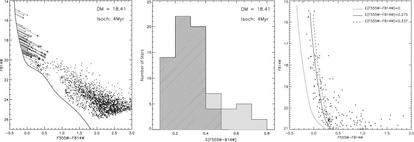
For every star we compute the intersection between the reddening vector and the isochrone, and we obtain, thus, the reddening value in terms of $E(F555W-F814W)$. Since the ACS photometric system is slightly different from the standard Johnson-Cousins system, we compute the exact reddening parameters for our ACS bands using the typical galactic extinction law of Cardelli et al. (1989), parameterized by a value of $R_{V}=A_{V}/E(B-V)=3.1$. We consider a set of template spectra taken from the NextGen catalog (Hauschildt et al., 1999), and we apply the extinction curve with an arbitrary $A_{V}$ which we choose to be equal to 1, and we measure the extinction $A_{F555W}$ and $A_{F814W}$ by means of integration of the original and reddened spectra within the ACS filter profiles. In this way we compute $R_{F555W}=A_{F555W}/E(F555W-F814W)\simeq 2.18$ and $R_{F814W}=A_{F814W}/E(F555W-F814W)\simeq 1.18$.

The derived reddening distribution, shown in Figure 6 (middle), appears to have a tail extended to higher values (filled histogram). This tail appears due to a number of UMS objects, which show a high color excesses. Taking into account all objects, including the ones with high color excess, the average reddening has a value $E(F555W-F814W)\simeq 0.34$ mag, corresponding to an optical extinction of $A_{V}=1.56$. However, these red objects are being suggested to be Herbig Ae/Be (HAeBe) stars (Gouliermis et al., 2002). Such stars of intermediate mass, aged between 1 and 10 Myr, occupy the faint end of the UMS with $17.5<F814W<20$ mag. Being in their pre-main sequence phase, they have an intrinsic color higher than that of MS stars in the same luminosity range. Consequently, if indeed these are not MS but HAeBe stars, which is possible due to the youthfulness of the system, then the derived reddening would be biased towards higher values.

We estimate the mean reddening without considering these stars (darker histogram in Figure 6 - middle) and we derived a lower mean value of $E(F555W-F814W)\simeq 0.275$ mag, corresponding to an optical extinction of $A_{V}=0.6$ mag. In Figure 6 (right) both values are applied to the 4 Myr isochrone model (the youngest available in the grid of models by the Padova Group). From this figure it is evident that the difference between the two values is not dramatic, producing more or less the same shift of the model in the CMD. As a consequence, and in order to avoid any biases due to the presence of young stellar objects in LH 95, we consider an optical reddening of $E(F555W-F814W)\simeq 0.3$ mag as the most representative for the region. We repeated the construction of the reddening distributions shown in Figure 6 (middle) and the determination of the mean reddening values using different isochrones, spanning an age range between 4 and 7 Myr and assuming different distances varying by 0.2 mag around the assumed distance modulus. We found that the mean reddening remains practically unchanged within 0.02 magnitudes, a difference small enough to confirm the accuracy of our estimation.

4. New set of observational PMS models

In the last decades several theoretical models for the pre-main sequence stellar evolution have been computed. Some of the most popular, for PMS masses above the hydrogen burning limit, are the models of Siess et al. (2000), Palla & Stahler (1999), D’Antona & Mazzitelli (1994, 1997) and Swenson et al. (1994). These models are generally expressed in terms of physical quantities, such as the effective temperature and the total bolometric luminosity, describing the evolution of stars in the HR diagram. However, one of the primary aims of stellar evolution theory is the explanation of the observed photometric data of stars in order to extract their masses and ages from their magnitudes and colors, and therefore a conversion between physical and observable quantities of the models is required. Such a conversion is specifically described by Siess et al. (2000), who include the transformation between $T_{\rm eff}$ and $L$ to colors and magnitudes in the $UBVRI$ Cousins system and $JHKL$ infrared bands for their models. These authors use simple relations $T_{\rm eff}$ versus color, as well as bolometric corrections from either Siess et al. (1997) or Kenyon & Hartmann (1995). These conversion tables, derived from observations of stellar clusters, are valid for solar metallicity dwarf stars, but the discrepancies can be significant when one deals with populations with different stellar parameters. In particular, the age of a star is related to the stellar radius and therefore to the surface gravity, which introduces differences in the spectral behavior, and therefore a population of different ages or metallicities may require different conversion relations. This issue can be important for e.g. cold M-type stars, for which the broad molecular absorption bands dominate the optical spectra, affecting integrated colors and color corrections.

Figure 7.— Distribution in the $T_{\rm eff}$, $\log{(g)}$ space of the synthetic spectra collected for our conversion of theoretical evolutionary models into the observable plane. The same spectra are used for metallicities of $[M/H]=0,\ -0.5,\ -1,\ -1.5$. Squares are spectra taken from the NextGen models of Hauschildt et al. (1999), while crosses are those of Kurucz (1979, 1993) (see § 4.1).

A more thorough method to analyze this issue is to make use of synthetic atmosphere models, performing photometry directly on synthetic spectra. Girardi et al. (2002) applied this method for their evolutionary models for evolved populations, which were converted in several photometric systems using a grid of atmosphere models described by three parameters ($[M/H]$, $\log{(T_{\rm eff})}$, $\log{(g)}$). This method was also applied for stars of sub-solar mass and brown dwarfs by Baraffe et al. (1998, 2001). For low- and intermediate-mass stars, however, there are no similar conversions of evolutionary models into the observable plane for various photometric systems available. As a consequence, and in order to have an accurate transformation of the PMS evolutionary models of Siess et al. (2000) into the observational plane, we apply a conversion of these models following an approach similar to that of Girardi et al. (2002). We construct, thus, observational models (both tracks and isochrones) for four assumed metallicities ($Z=0.02$, $0.01$, $0.008$, $0.004$) and several photometric systems (specifically Johnson, Cousins, HST WFPC2, HST ACS, HST STIS, HST NICMOS, Galex, Strömgren, SDSS, Tycho and 2MASS).

Figure 8.— Comparison of the evolutionary models for PMS stars developed in this work with the ones by Siess et al. (2000). Left: Color-Color Diagram of isochrones from the models of Siess et al. (2000) for the ZAMS and ages of $0.1$, $0.3$, $1$, $3$, $10$, $30$ Myr for $Z=0.02$. The dotted line refers to the original Siess et al. (2000) isochrones, in which a unique temperature $-$ color relation is used, while the solid lines are the results of our analysis. The differences between the two treatments are mostly evident at larger colors, at about $T\sim 4000K$, where M-type optical spectra are dominated by oxide bands, and are strongly dependent on age due to variations in the surface gravity of the stars. Right: Comparison between the original isochrones of Siess et al. (2000) for $Z=0.02$ and our treatment in the $(V-I)$, $I$ diagrams. For medium masses (top left region) the differences are negligible, while for low-mass, cold stars the shifts are important. In particular it is evident that our transformations extend to larger colors than those of Siess et al. (2000).

4.1. The Method

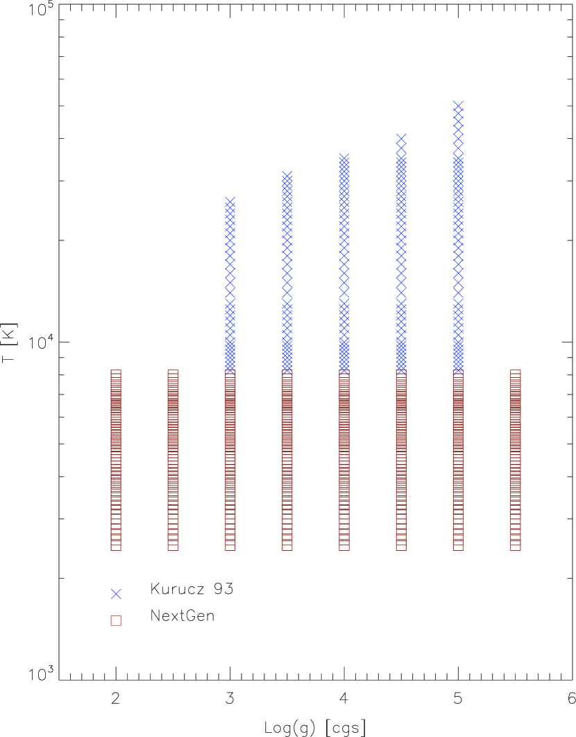
We apply our conversion method first by collecting a grid of atmospheric models in the $T_{\rm eff}$, $\log{(g)}$, $[M/H]$ space. These models are shown in Fig. 7. We selected spectra from NextGen (Hauschildt et al., 1999) for low- and medium-temperature stars. The selected grid covers temperatures 2600 K $\leq T_{\rm eff}\leq$ 8200 K in steps of 200 K and surface gravities $2.0\leq\log{(g)}\leq 5.5$ in cgs units, spaced in 0.5 dex. For higher temperatures we used the grid of models by Kurucz (1979, 1993), with gravities $\log{(g)}$ between $3.0$ and $5.0$. This grid covers entirely the range of stellar parameters in the evolutionary models of Siess et al. (2000). The considered metallicities cover the values $[M/H]=0.0,\ -0.5,\ -1.0,-1.5$, representative of stellar populations in the Magellanic Clouds, as well as in many regions of the Galaxy. We re-sampled the NextGen models, the resolution of which is much higher than required for our purposes of broad-band synthetic photometry, to the wavelength values of the Kurucz models, and we normalized them to the same units (erg cm^-2 s^-1 Å^-1).

The absolute magnitude in a photometric band $S_{\lambda}$ of a star with a spectral energy distribution $F_{\lambda}$, and stellar radius $R$ is given by

$$M_{S_{\lambda}}=-2.5\log\bigg{[}\bigg{(}\frac{R}{10\textrm{pc}}\bigg{)}^{2}\frac{\displaystyle\int_{\lambda}\lambda F_{\lambda}S_{\lambda}10^{-0.4A_{\lambda}}\textrm{d}\lambda}{\displaystyle\int_{\lambda}\lambda f^{0}_{\lambda}S_{\lambda}\textrm{d}\lambda}\bigg{]}+ZP_{S_{\lambda}}$$ (5)

where $f^{0}_{\lambda}$ is a reference spectrum that gives a known apparent magnitude $ZP_{S_{\lambda}}$; in the Vegamag photometric system, which uses the flux of $\alpha$ Lyr as reference, $f^{0}_{\lambda}=F_{\lambda,{\rm VEGA}}$ and the zero-points $ZP$ are close to zero.

We assume an extinction $A_{\lambda}=0$, since we are interested in constructing a general observable grid of evolutionary models for unreddened objects. Eq. (5) can be written then as:

$$M_{S_{\lambda}}= -5\log\bigg{(}\frac{\displaystyle R_{\odot}}{\displaystyle 10{\rm pc}}\bigg{)}-5\log\bigg{(}\frac{\displaystyle R_{\star}}{\displaystyle R_{\odot}}\bigg{)}+B(F_{\lambda},S_{\lambda})$$

$$= 43.2337-5\log\bigg{(}\frac{\displaystyle R_{\star}}{\displaystyle R_{\odot}}\bigg{)}+B(F_{\lambda},S_{\lambda})$$ (6)

where

$$B(F_{\lambda},S_{\lambda})=-2.5\log\bigg{(}\frac{\displaystyle\int_{\lambda}\lambda F_{\lambda}S_{\lambda}\textrm{d}\lambda}{\displaystyle\int_{\lambda}\lambda F_{\lambda,VEGA}S_{\lambda}\textrm{d}\lambda}\bigg{)}+ZP_{S_{\lambda}}$$ (7)

The latter term can be directly calculated having the synthetic spectrum of any considered star, a calibrated Vega spectrum, the band profile of the photometric filter considered and the eventual zero-point $ZP$. For the computation of $B$ we used the Gensynphot code included in the Chorizos package (Maíz-Apellániz, 2004). Given a set of stellar parameters ($T_{\rm eff}$, $\log{(g)}$, and $[M/H]$) for a sample of points (stars) on an evolutionary track or an isochrone, the corresponding spectra are computed by interpolation on the Cartesian grid of synthetic models of stellar atmospheres. Then, the integral at the numerator of Eq. (7) is computed. The final normalization is performed using a recent reference spectrum of Vega (Bohlin, 2007) with the corrected zero-points as reported by Maíz-Apellániz (2007).

Following this method we converted all the original evolutionary models of Siess et al. (2000) into absolute magnitudes, for the metallicities of $Z=0.02,\ 0.01,\ 0.008$ and $0.004$ corresponding to $[M/H]\simeq 0.0,-0.3,\ -0.4,\ -0.7$ respectively. Considering that the original Siess et al. models were computed only for $Z=0.01$ and 0.02, we extrapolated the theoretical isochrones computed for $Z=0.01$ to lower metallicities with the use of the atmosphere models computed for such metallicities. Naturally, a more detailed treatment of low-metallicity tracks and isochrones requires both evolutionary and atmospheric models to be available at the same considered metallicity. However, for the present analysis in the LMC, for which $Z\sim 0.008$, the uncertainties are quite low given the small difference between the metallicity of the theoretical isochrones (0.01) and that of the atmosphere models (0.008).

4.2. Comparison with previous conversions

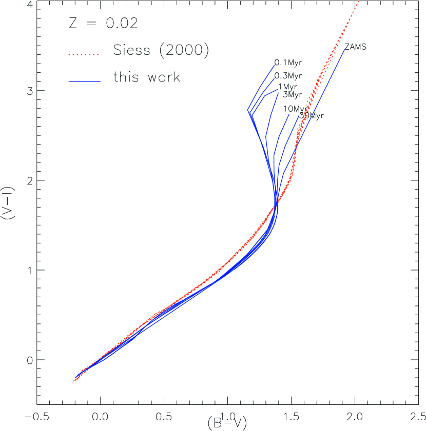
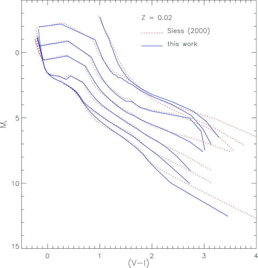
With our construction of the observational plane for PMS evolutionary models, we verified that a single temperature-color relation is not sufficient for stars with different physical parameters, especially surface gravity. In Figure 8 (left) we present a comparison between the $(B-V)$, $(V-I)$ color-color diagrams for different isochrones, as they were derived from the method of Siess et al. (2000) (red dotted lines) and from our method with the use of atmosphere models (blue continuous lines). In this figure it is shown that the isochrones of Siess et al. (2000) are distributed along one single sequence, due to the use of monolithic temperature-color relations, which are independent of the surface gravity. However, our observational isochrones show a spread for high color terms (low $T_{\rm eff}$), because differences in ages imply differences in the surface gravities, which produce variations in the integrated colors according to the atmosphere models we used. The major differences arise for M-type stars, in which the optical spectra are dominated by strong oxide absorption bands. Figure 8 (right panel) shows these differences on the CMD. As shown in this figure, the differences between our method and that of Siess et al. (2000) are mostly evident at the red end of the models, where our computations predict redder colors, and for the youngest models, where the stellar surface gravities are lower than those for main sequence stars. In Figure 8 the example of $Z=0.02$ is shown.

5. The Initial Mass Function

The mass function (MF) is defined as the number distribution of stars as a function of mass. While a general observational approach measures the so called Present Day Mass Function (PDMF), a cornerstone for understanding how stars form is the Initial Mass Function (IMF), which is the mass distribution according to which stars are born. For a pre-main sequence population younger than the time required by the most massive stars to disperse it, or to evolve into post-MS evolutionary phases, the observed mass function coincides with the IMF.

Generally, the IMF is parameterized as follows:

$$\xi(M)~{}\textrm{d}M\propto M^{-(1+x)}$$ (8)

namely, approximating it with a power-law (e.g. Salpeter, 1955) or with a series of power-laws, with exponents changing in different mass ranges (Scalo, 1986; Kroupa, 2002). In this section we describe the “average” IMF derived for the stellar populations of the central region of LH 95, as it has been defined in § 3.2.

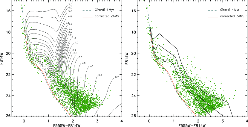
The $F555W-F814W$, $F814W$ CMD of Figure 5 (right panel) is shown again in Figure 9, with our observable PMS evolutionary tracks (left panel) and three indicative PMS isochrones (right panel), computed in § 4, overlayed. In the right panel of the figure the ZAMS from our grid of models is also plotted along with the youngest MS isochrone from the Padova grid of evolutionary models (Girardi et al., 2002) corresponding to $\log{\tau}\simeq 6.6$. Both isochrones fit to each other very well demonstrating that the bright MS stars of LH 95 have ages of  $\sim$$<$  4 Myr. As far as the PMS stars of LH 95 concerns, their positions in the CMD corresponds to an age-spread that covers ages between $\sim$ 1.5 and 10 Myr according to our PMS models. A simple statistics on the distribution of the ages of these PMS stars, based on their CMD positions, results to a normal distribution of ages which peaks at about 4 Myr. However, if this age-spread is true or not can be the subject of debate, as we discuss in § 3.3. Therefore, based on the PMS population of LH 95 we define an indicative age for LH 95 of $\log{\tau}=6.6\pm 0.4$. Corresponding PMS isochrones for ages of 1.5, 4 and 10 Myr from our grid of observable PMS models are overlayed on the CMD in the right panel of Figure 9. A comparison of this age, which also represents the individual subclusters of LH 95, with the corresponding dynamical crossing time, estimated in § 3.2, shows that all sub-clusters, as well as the whole central region have an age comparable to their crossing times, indicating that these systems are under ‘mixing’ process if not already ‘mixed’ and therefore we probably do not observe them close to their initial morphology.

Figure 9.— The CMD of the cluster area of LH 95 with PMS evolutionary tracks (left) and isochrones (right) overlayed for a distance modulus $m-M=18.41$ mag and a mean reddening of $E(F555W-F814W)=0.275$ mag (see § 3.4). The PMS tracks and the corresponding PMS isochrones and ZAMS are computed by us for the ACS filter system, and for the metallicity of the LMC (§ 4). The 4 Myr isochrone for evolved MS stars is from the Padova grid of evolutionary models (Girardi et al., 2002). The comparison of this isochrone with our ZAMS demonstrates that it practically corresponds to the youngest MS populations. The selected PMS isochrones overlayed in the right panel have ages of 1.5, 4 and 10 Myr. The central, 4Myr, corresponds to the the mean age of the observed PMS stars, where the other two delimit the 1$\sigma$ width of the broadening of these stars in the CMD.

5.1. Construction of the IMF

Based on our new set of PMS models computed above for the ACS photometric bands and the average LMC metallicity ($Z\sim 0.008$), we assigned a value of mass to all the stars identified in the region of LH 95, by comparing our observed data with the evolutionary tracks of these models. For this comparison we assumed a distance modulus of $m-M=18.41$ mag, and an average reddening of $E(F555W-F814W)=0.275$ mag, as it is derived in § 3.4. According to Figure 9, our photometry reveals PMS stars with masses as low as 0.2 M_⊙. Our sample, though, as we discuss later, is complete for masses down to $\simeq$ 0.43 M_⊙. For the PMS stars we assign a mass measurement to each observed star according to their positions in the CMD by interpolating between the PMS evolutionary tracks shown in Figure 9.

The position of the brightest main sequence stars is not covered by our PMS evolutionary models, limited for masses below 7M_⊙. Therefore, we derive the masses of these stars directly from the Padova 4 Myr isochrone – already used for the determination of the average reddening in § 3.4 – shifted in the direction of the reddening vector to reach individually each one of these stars. The good agreement between this Padova isochrone and the corrected ZAMS from the Siess models is evident from Figure 9. While we de-redden the most massive MS stars according to their individual position in the CMD, their mass estimation is based solely on photometry. A more accurate estimation of the mass for massive stars certainly requires spectroscopy, because for such hot stars the broad-band colors are degenerate (Massey et al., 1995), and naturally this effect may influence the mass estimation for the brightest MS stars in our sample and the corresponding IMF. We discuss the influence of the use of photometry alone to the slope of the derived IMF in §5.2.

With the masses of both the MS and the PMS stars in our sample available the construction of their IMF is in principle straightforward, by binning the stars according to their masses and fitting the derived distribution. However, there are considerations, which affect the construction and interpretation of the IMF, and which should be taken into account. We discuss these issues below.

• An important issue to be considered is the decontamination process of the stellar sample in the region of the association from the field populations. The Monte Carlo method for the field subtraction, as applied in § 3.3, is based on probabilities and therefore it is a stochastic process. As a consequence, the number of stellar members of the system, which are counted in an arbitrary mass bin is not determined in an unambiguous manner. Moreover, the statistical significance of this number is not determined by the fraction of stars considered as system members over the total number of stars, but it depends also on the probability that all the observed stars in the bin are system members. This dependence affects specifically the MS populations with 19  $\sim$$<$  $m_{\rm F814W}$/mag  $\sim$$<$  22, which as it is shown in Figure 5 are well mixed with field populations, implying a higher uncertainty in the determination of the fraction of system members. In the faint part of the CMD, system and field populations are in general well distinguished, and therefore the uncertainties in the numbers of PMS stars that are true system-members are insignificant. However, there is an important possibility that a fraction of the binary sequence, evident in the CMD for the LMC field population (see Figures 5 and 9), contaminates the selected sample of PMS star-members of the system. We consider this bias and report on its effect in § 5.2

• The fitting process of the IMF. Typical linear regression methods, which are used for obtaining a functional form of an observed IMF, such as the $\chi^{2}$-method, consider the presence of measurement errors and are based on the assumption that the uncertainty associated to each point follows a Gaussian distribution. However, in this case the uncertainty in the number of counts within a mass bin is the overall effect of both the Poissonian error that naturally comes from the counting process, and the uncertainty that arises from the field subtraction, as discussed above. Although the first can be well approximated with a Gaussian for large $n$, the latter depends on the positions of stars and tracks in the CMDs. Moreover, in the high mass regime, where the number statistics is poor, the Poissonian error cannot be treated as Gaussian, requiring the asymmetry of the distribution to be taken into account.

• The completeness-correction process. In the low-mass regime corrections for the incompleteness of the stellar sample are required to estimate the actual number of stars. However, given the width of the low-mass evolutionary tracks in the CMD shown in Figure 9 and the 2-dimensional variation of the completeness itself in the CMD (in both magnitudes and colors; see § 2.1), this correction is not unique for all the stars counted in a considered mass bin.

We construct the system IMF of the association LH 95, with a special care in addressing the above issues, as follows. We first determine a grid of logarithmic mass bins, for which we choose variable width in $\log(M)$, that increases from $0.04$ dex at low masses to $0.25$ dex for the higher masses. The counting of the stars is made in variable-sized bins because such bins yield very small biases, which are only weakly dependent on the number of stars, in contrast to uniformly binned data (Maíz-Apellániz & Úbeda, 2005). For each $i^{\rm th}$ bin a number of stars $N_{i}$ is derived. In order to achieve a statistically correct sampling of points for the constructed IMF, we simulate for each bin the probability distribution expected for every $N_{i}$ with a sample of 1000 points randomly selected from a Poisson distribution with mean $N_{i}$.

We then consider the position in the CMD of all the stars in each bin, and we compute for each star its completeness $C$ (the ratio between the number of sources detected and the total number of sources) as a function of both magnitude and color according to the completeness measurements described in § 2.1, for the central region of LH 95. Let us consider the $j^{\rm th}$ star counted in the $i^{\rm th}$ bin. The star is located in a specific position of the CMD, where completeness is $C_{j}$, meaning that the total number number of stars corresponding to $j$ is simply $1/C_{j}$. Consequently, for the total number of stars counted in the bin, $N_{i}$, the completeness correction is:

$$F_{i}=\frac{\displaystyle\sum_{j}^{N_{i}}\frac{\displaystyle 1}{\displaystyle C_{j}}}{\displaystyle N_{i}}$$ (9)

which is a quantity $\geq 1$.

We multiply our Poissonian sample associated to each $i^{\rm th}$ bin by $F_{i}$, and we divide by the width of the bin in order to express numbers in units of number of stars per solar mass. In order to take into account the additional error introduced by the stochasticity of the Monte Carlo field-subtraction (§ 3.3), we iterate the technique of field removal $200$ times, each time repeating the procedure explained in the previous paragraphs, namely, counting the $N_{i}$ number of stars in each $i^{\rm th}$ bin, sampling a Poisson random population associated to it, and computing and applying the completeness correction.

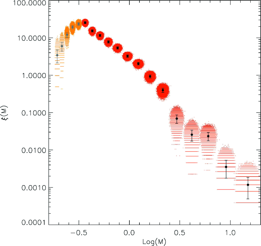
The outcome of this approach is that for each mass-bin, instead of a single point-error combination, we have a population of 200,000 random IMF points, derived according to the true statistical distribution of the expected number of stars in the bin. Clearly, the mean and the standard deviation of each of these distributions represent the IMF data points and error bars. The main advantage of this technique is that we override the non-Gaussian behavior of the mass-bin error bars. Specifically, now for every mass-bin we do not have one point associated with an error that cannot be treated by the regression theory, but a numerous set of points with no uncertainties associated to them, and consequently with arbitrary equal weights for all mass-bins. Naturally, this allows a more accurate fitting of the mass function.

In Figure 10 we visualize the concept of this approach. For every mass-bin the set of random points, representing the distribution of the expected $\xi(M)$ is drawn with tiny colored dots. In this plot an artificial spread along the $x$-axis (a random Gaussian shift with $\sigma=1/8$ of the bin width) is introduced to better highlight the distributions along the $y-$axis. The black dots with error bars show the average and standard deviation of each sample of points. The derived numbers are reliable for $M$  $\sim$$>$  0.35 M_⊙, whereas for the lower masses (first five mass bins from the left) the completeness corrections are not sufficient. This limitation is evident from the CMD of Figure 9, where it can be seen that for the evolutionary tracks for very low masses ($M$  $\sim$$<$  0.35 M_⊙), the completeness is extremely low, so that no stars can be detected, limiting the ability to recover the true number distributions for such masses.

Figure 10.— The system IMF plot of LH 95, which demonstrates our method for treating the distribution of the expected number of stars per mass-bin according to uncertainties due to counting, incompleteness and field subtraction. Each mass-bin is represented by the distribution along the $y-$axis of a set of 200,000 randomly selected points, which map the true statistical uncertainties of star counts. An additional Gaussian spread with $\sigma=1/8$ of the bin width along the $x-$axis has been artificially added for each bin to better highlight the behavior of the individual distributions. The asymmetry of the statistical distributions especially for the high-mass end of the IMF is demonstrated by the drop-like shape of the distributions. The very-low mass end (light-gray points) appears to drop due to the limitation of our completeness correction technique in CMD regions where no stars are detected. Units of the IMF are number of stars per solar mass per pc² .

5.2. IMF model fitting

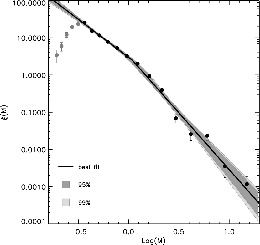
A commonly used procedure to derive the functional form of an observed IMF is to fit a predefined function to the individual numbers of stars originally counted per mass-bin taking into account the corresponding counting errors. However, in our case, we have simulated the statistical distribution of $\xi(M)$ per mass-bin taking into account the additional errors due to incompleteness and field subtraction. Within our statistical approach we perform 200 repetitions of the Monte Carlo field subtraction method and for each of them we map the Poissonian statistics 1000 times. The outcome is a non-analytical probability distribution for each mass-bin that represents the true expected statistical uncertainties due to the issues discussed in §5.1. This process provided a large sample of 200,000 points per mass-bin, and naturally the best-fitting function can be derived more accurately with the use of these data, rather than the original 14 bins. The only assumption that we make is that the functional form of the IMF of LH 95 can be correctly represented by power-laws, according to the parameterization given in Eq. (8), and therefore we search for the best multiple power-law which may reproduce our data. As seen in Figure 10 the IMF seems to be more shallow for the low masses ($M\lesssim 1$ M_⊙) than for intermediate and high masses, implying that it could be reproduced by a two-phase power-law. We investigate, however, whether a two-phase power-law is sufficient or a three-phase power-law, such as that proposed by Scalo (1998), is required to represent our IMF.

In order to find the best fit of two- and three-phase power-laws to our IMF we applied a Levenberg-Marquard non-linear least square minimization technique (Levenberg, 1944; Marquardt, 1963). For this fit we consider only the mass-bins of the IMF for which the completeness correction allowed us to reconstruct the actual number of stars, meaning for $\log{(M/{\rm M}_{\odot})}>-0.5$. The slopes of the power-laws, as well as the position of the break points along the abscissa are the free parameters of our fit algorithm. All 200,000 points of each mass-bin are considered of equal weight. However, since a two-phase power-law is a sub-case of the three-phase power-law, the sum-of-squares of the latter is always lower. Therefore, the results of the fit algorithm for each case are normalized in a rigorous manner by performing the so-called statistical “F test”.

This test compares the relative increase in the residual sum of squares by reducing the complexity of the model with the relative increase of degrees of freedom, namely, the differences between the number of data points and the free parameters. Factor $F$ is, thus, computed as

$$F=\frac{\textstyle\frac{\textstyle RSS_{2}-RSS_{3}}{\textstyle p_{3}-p_{2}}}{\textstyle\frac{\textstyle RSS_{3}}{\textstyle n-p_{3}}}$$ (10)

where $RSS_{2}$ and $RSS_{3}$ are the residual sum of squares for the two- and three-phase power-law best fit models, $p_{2}=4$ and $p_{3}=6$ are the corresponding number of free parameters, and $n$ the total number of points, which, in our case, is the effective number of considered mass bins (14) and not the total number of variables used in the fit (200,000 $\times$ 14), given that the additional multiplicity has been introduced to map the non Gaussian errors. Typically, if the simpler model is valid (which means that there is no need to add parameters), then $F\simeq 1$, whereas if the complex model represents the distribution better, then $F\gg 1$. We obtain $F=1.15$. The probability, $P$, that the null hypothesis, which is “the improvement found adding additional parameters is solely due to chance” (or “the simpler model is good enough”) should be rejected is given by the value of the cumulative Snedecor’s $F$ distribution with $(p_{3}-p_{3},n-p_{3})$ degrees of freedom. In our case it is $P=0.65$, while, generally, a value of $P>0.95$ is required to state with sufficient significance, that the complex model is better. Under these circumstances, we conclude that our system IMF is best approximated by a two-phase power-law.

We compute the uncertainty associated to this result, by utilizing a sampling technique. For each mass-bin we pick randomly one out of the 200,000 points from the corresponding distribution of $\xi(M)$ in that bin, and we perform a two-phase power-law fit as described above, obtaining the two measurements for the slope, and the point ($\log{M}$, $\log{\xi(M)}$) where the change of the slope occurs. After repeating this process for a substantial amount of times, we obtain a statistically significant sample for the values of the two slopes and the point of change, and consequently the relative confidence level of our fit. Figure 11 shows the result of our fit to the system IMF of LH 95. The best two-phase power-law fit is shown as a solid line, while the uncertainty of this fit is demonstrated by the grey shaded areas for confidence of 95% (dark grey) and 99% (light grey) respectively. In Table 3 we give the system IMF slopes $x$ and their uncertainties with the corresponding mass ranges. The 1$\sigma$ error in the determination of the break point is 0.07 dex.

Another bias that should be considered in the construction of the system IMF of LH 95 is the possible contamination of our selected sample of PMS stars by a binary sequence of the LMC field MS population, discussed in § 5.1. In order to quantify the effect of this bias we select this part of the CMD and remove the corresponding stars. Specifically, we remove all stars bluer than the borders defined by the points (F555W$-$F814W, F814W) $=$ (0.9, 22.9), (1.65, 24.3) and (2.2, 26.9) on the CMD. The number of these stars changes according to the stochastic Monte Carlo field subtraction; on average they count to 82 members, less than 4% of the selected PMS population. Then, we reapply the analysis described in §§ 5.1 and 5.2 for the construction and model-fitting of the system IMF. We find that this new IMF does not differ significantly from the one shown in Figure 11, and its shape is not different from that described with the slopes of Table 3. Specifically, this IMF has 99%-confidence slopes $x\simeq 1.16$ for $-0.5<\log(M/{\rm M}_{\odot})<0.04$, and $x\simeq 2.03$ for $\log(M/{\rm M}_{\odot})>0.04$, indistinguishable from the slopes of Table 3. Our analysis on the sub-clusters of LH 95 showed that the contamination of our sample by a MS binary sequence does not alter also the shape of their individual system IMFs, with slopes as well indistinguishable from those given in Table 4.

The lack of spectroscopy and the use of broad-band photometry alone for the mass estimation of massive MS stars is found to lead to steeper IMF slopes (Massey et al., 1995), and this may affect the overall intermediate- and high-mass slope of the IMF of LH 95. However, considering that in their analysis Massey et al. (1995) show that this effect is significant for stars more massive than 15 M_⊙, the only mass-bin in our IMF that can be biased is the most massive one, comprising stars with $11$  $\sim$$<$  $M$/M_⊙  $\sim$$<$  $20$. In addition, the IMF derived from photometry alone for high-mass stars in star-forming regions of the Magellanic Clouds is found to be also quite shallow and not steep, and within the observed IMF slope variations in such regions (see discussion in §6.2). Under these circumstances, the corresponding uncertainty in our derived system IMF slope due to the use of photometry alone should not be expected to be larger than those given in Table 3.

Figure 11.— The system IMF of the association LH 95. The best two-phase power-law fit derived in § 5.2 is drawn with a solid line, while the shaded areas represent the $95\%$ and $99\%$ confidence uncertainties in the slope determination and the break point. Units of the IMF are logarithmic number of stars per solar mass per pc². The corresponding IMF slopes and their uncertainties are given in Table 3.

Table 3The slope of the system IMF of the association LH 95

mass range	$x$	$\sigma_{95\%}$	$\sigma_{99\%}$
$-0.5<\log(M/{\rm M}_{\odot})<0.04$	1.05	${}^{-0.20}_{+0.15}$	${}^{-0.29}_{+0.20}$
$\log(M/{\rm M}_{\odot})>0.04$	2.05	${}^{-0.28}_{+0.39}$	${}^{-0.32}_{+0.53}$

Note. — A Salpeter (1955) IMF would have a slope of $x=1.35$.

6. Discussion

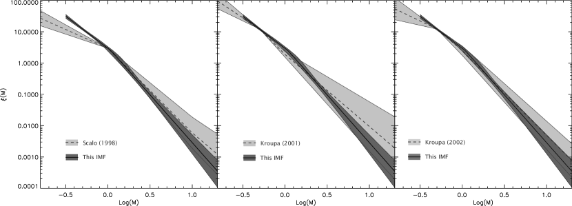
The IMF constructed in the previous section is the most complete extragalactic system IMF down to the sub-solar regime derived so far. Specifically, our correction for incompleteness in the derivation of $\xi(M)$ actually provides a reliable IMF down to $M\simeq 0.43M_{\odot}$, as discussed in §5.1. Probably, the most interesting result concerning this IMF is the change in its slope, which we verified statistically for stars in the the subsolar mass range. The IMF slope, $x$, decreases for these stars by one unit. An analogous behavior is generally found in related studies in the Galaxy. Comprehensive studies which summarize the average properties of the galactic IMF are those of Scalo (1986), revisited in Scalo (1998) and Kroupa (2001, 2002). The latter investigations are rather complete, since they cover stellar mass distributions in a wide mass range, from brown dwarfs with $M\sim 0.01M_{\odot}$ to the most massive stars. According to Kroupa (2002), the IMF slope $x$ (Eq. 8) changes from $x=-0.7$ in the sub-stellar mass range, to $x=0.3$ for masses between 0.08 M_⊙ and 0.5 M_⊙, $x=1.3$ for 0.5 M_⊙ $<M<$ 1 M_⊙, and $x=1.7$ for stars of higher masses. This IMF is generally characterized as the Galactic average, in the sense that it is reasonably valid for different regions of the Galaxy. A comparison between the system IMF we construct here for LH 95 and that of Scalo (1998), as well as the universal IMF of Kroupa (2001) and the average Galactic IMF of Kroupa (2002), is shown in Figure 12. We scaled all other IMFs to match our mass distribution at $\log(M/{\rm M}_{\odot})=-0.3$. In Figure 12 an overall agreement between the various IMFs is quite evident.

The mass limit of the breaking point in our system IMF ($\sim$ 1 M_⊙) coincides with the “standard Galactic field IMF”, which has been reported to have a change of slope at $1M\mbox{${}_{\normalsize\odot}$}$ (Kroupa, 2002), in agreement also with the knee of the IMF derived by Scalo (1998). In addition, there is a second knee in the Kroupa IMF, which occurs at the lower mass-limit of 0.5 M_⊙. Since we cannot constrain the system IMF below $0.43M\mbox{${}_{\normalsize\odot}$}$ we do not identify this second knee. The slope of our IMF for stars with $M$  $\sim$$>$  1 M_⊙ falls within the range of slopes found by both Scalo and Kroupa. This is in line with the recent finding that the system IMF is essentially equal to the stellar IMF for intermediate and massive stars (Weidner et al., 2008). Our system IMF, however, is somewhat steeper, as an indication of a bottom-heavy IMF, but the use of photometry alone for the estimation of the masses for the brightest stars ($M$  $\sim$$>$  15 M_⊙) may bias the slope to steeper values (see §5.2). As far as the slope of our IMF in the sub-solar regime is concerned, it is found slightly more shallow than that of these authors. Specifically, our IMF is by $\Delta x=0.1$ - $0.3$ more shallow than the stellar IMF (as seen from the theoretical $\alpha$-plots of Kroupa, 2001), making the resulting stellar IMF for LH 95 indistinguishable to the Galactic-field stellar IMF (e.g. Kroupa, 2002). It should be noted that both Scalo and Kroupa IMFs extend down to masses as low as the hydrogen burning limit ($M\simeq$ 0.08 M_⊙), well below our detection limit. In general, one can conclude that the system IMF we derive for LH 95 is in agreement with the average galactic IMF in the entire mass range we studied, from 0.43 M_⊙ to $\sim$ 20 M_⊙.

Figure 12.— Comparison between the derived LH 95 system IMF and the average IMF of Scalo (1998) (left), Kroupa (2001) (middle), as well as the universal IMF of Kroupa (2002) (right).

The high-mass IMF of LH 95 was constructed earlier from direct CCD imaging in $BVR$ with the 1-m telescope at Siding Spring Observatory by Gouliermis et al. (2002). These authors provide the field-subtracted completeness-corrected IMF of the system for stars with masses down to $\sim 2$ M_⊙, and they find that this IMF can be fitted with a single power-law with slope $x=1.2\pm 0.3$ for stars with masses up to about 17 M_⊙. This result indicates a more shallow slope $x$ than what we found for intermediate and high mass stars ($x=2.05$). However, in our analysis we included masses as low as $1M_{\odot}$, extending the mass range investigated in Gouliermis et al. (2002). Indeed, if we exclude the mass bins from 1 to 2 M_⊙ ($0<\log{(M/{\rm M}_{\odot})}<0.3$) from our analysis we derive a more shallow value for $x$ for the intermediate- and high-mass stars. The effect of a steeper IMF for the mass range between 1 and 2 M_⊙ is evident in Figs. 10 and 11. After excluding stars of $M<2$ M_⊙ from the considered stellar sample and performing a single power-law fit on the resulting $\xi(M)$, we find an IMF slope of $x\simeq 1.55$, comparable to that of Gouliermis et al. (2002).

Concerning our derived IMF for the central region of LH 95 it is important to assess the accuracy of our findings, in relation with the possible sources of uncertainties. One of the most important error sources normally comes from the incomplete stellar samples. However, in our case we consider the completeness as it has been derived from artificial star tests in the central part of LH 95, where the crowding is higher (Figure 2b), and we performed rigorous corrections for incompleteness taking into account variations of completeness for all stellar positions in the CMD. As far as the very-low mass stars is concerned, we do not consider those with $M$  $\sim$$<$ 0.35 M_⊙, where our completeness correction is limited.

6.1. Stellar Binarity

An important source of uncertainty in the construction of the IMF is also the presence of unresolved binaries. Unresolved binarity, can modify the shape of the observed mass function so that it appears more shallow than what it actually is. For this reason, we stress that the IMF reported in Table 3 must be considered as the system IMF of our region, and not a stellar IMF as which one refers when the effect due to binarity is removed. Clearly it is not possible to correct this effect without the knowledge of the actual binary fraction of the studied population, but one can estimate the overall effect on the final mass distribution. Sagar & Richtler (1991) applied Monte Carlo simulations on artificial stellar populations, in order to investigate the change in the mass function slope $\Delta x$ due to binarity for stars in the mass range $2<M/M\mbox{${}_{\normalsize\odot}$}<14$. These authors found that the result depends on both the binary fraction $f$ and the original slope $x_{0}$ of the mass function. Specifically, for an original slope $x_{0}=1.5$ and a binary fraction $f=0.5$ Sagar & Richtler (1991) found a slope change $\Delta x\simeq 0.34$, while for $x_{0}=0.5$ and $f=0.5$, $\Delta x\simeq 0.5$. On the other hand, Kroupa et al. (1991) in their investigation on the low-mass IMF in the solar neighborhood, showed that binaries can make a major effect in mass function determinations below 1 M_⊙. Consequently, the expected changes in the slope due to unresolved binarity may introduce uncertainties in the derived slopes given in Table 3, but not large enough to justify the intrinsic change of slope that we observe in our IMF for LH 95 at 1 M_⊙. In any case, as discussed by Kroupa (2002), most of the studied mass functions in the literature are not corrected for binarity, mostly due to the high uncertainty in the binary fraction. The Galactic IMF derived by (Kroupa, 2001, 2002), however, has been corrected for unresolved multiple systems. A more recent study of the binary effect on the massive-star IMF by Weidner et al. (2008) shows that a power-law IMF is not significantly affected even by large numbers of unresolved binaries or higher order multiples.

In order to analyze the effect of unresolved binarity in the measured slope of the system IMF in the sub-solar regime, we apply a Monte-Carlo technique adopted from the work of Sagar & Richtler (1991) and Kroupa et al. (1991, 1993). For this method we assume a pre-defined set of functions for the IMF, and in order to be consistent with those we find for the system IMF, as well as with the Galactic IMF of Kroupa (2002), we consider three-phase power laws with break points at 0.3 M_⊙ and 1 M_⊙. We limit our mass samples in the stellar regime with $M>$ 0.08 M_⊙. We let the slopes $x_{1}$, $x_{2}$, $x_{3}$ within the three selected mass ranges to change respectively in the range $-1<x_{1}<1.5$ for $0.08<M/{\rm M}_{\odot}<0.3$, $0<x_{2}<2$ for $0.3<M/{\rm M}_{\odot}<1$ and $1<x_{3}<2$ for $M/{\rm M}_{\odot}>1$. For each of these mass distributions, we generate a sample of 50,000 stars positioned in the CMD along our 4 Myr PMS isochrone (corresponding to the age of the system). We assume binary fraction, $f$, between 0 and 1, and we randomly pair couples of stars from the simulated distributions. We then compute the new position in the CMD of these binary systems and assign new masses as if they were single stars. The out-coming mass distributions are fitted with a 3-phase power law imposing the same position of the break points.

We isolate the models for which the derived system IMF in the range $0.3<M/{\rm M}_{\odot}<1$ is compatible with the one measured for LH 95 within the confidence interval of the latter. Naturally there are multiple solutions, given the lack of knowledge about the actual IMF of LH 95, its shape at lower masses, and the binarity fraction appropriate for this system. However, we can constrain the uncertainties due to unresolved binarity in our measured slope, $x_{2}$, for the subsolar regime $0.3<M/{\rm M}_{\odot}<1$. The IMF slope within this mass range is mainly affected by the value of $f$. If we assume $x_{1}$ to be that of the Galactic-field IMF, the slope $x_{2}$ in this mass range changes by $\Delta x_{2}\simeq 0.45$ for $f=1$. This change decreases to $\Delta x_{2}\simeq 0.35$ for $f=0.6$, and $\Delta x_{2}\simeq 0.25$ for $f=0.4$.

A change in the original IMF for masses larger than Solar does not affect our results by more than $\Delta x_{3}=0.1$, whereas changing the slope at very low masses ($0.08<M/{\rm M}_{\odot}<0.3$) affects significantly the slope $x_{2}$, diminishing it when $x_{1}$ becomes much steeper or shallower than the value of Kroupa (2002) IMF. Even in this case, the effect is always less than $\Delta x_{3}=0.2$. Therefore, we conclude that for a reasonable binary fraction of $f\simeq 0.5$, unresolved binarity can bias our IMF slope, $x$, in the subsolar regime on average by no more than 0.3 units. As a consequence unresolved binarity does not affect significantly the measured IMF for LH 95 within the estimated errors, and thus the corrected stellar IMF for LH 95 remains indistinguishable from the Galactic IMF.

6.2. Metallicity effects

Recent findings suggest that variations in the metallicity of a star-forming cloud might cause variations in the IMF slope for stars with masses $M<0.7$ M_⊙, in the sense that Galactic regions with higher $[Fe/H]$ appear to produce more low-mass stars (Kroupa, 2002). This is further supported by the measured IMF in Galactic open clusters (Barrado y Navascués et al., 2001), globular clusters (Piotto & Zoccali, 1999) and old and relatively metal-poor thick disk stars (Reylé & Robin, 2001). Kroupa (2002) proposes a systematic metallicity dependence of the IMF exponent of the form $x\approx 0.3+\Delta x[Fe/H]$, where $\Delta x\approx 0.5$. If we apply this dependence to the LMC, for which $[Fe/H]\simeq-0.4$, we find that the slope of the average IMF in the LMC for masses $M<0.7$ M_⊙ should be flattened to the value $x\approx 0.1$. The flattening of the IMF of the LMC general field for stars with $M<0.7$ M_⊙ has been discussed by Gouliermis et al. (2006a), who found only indications of such a change in the IMF slope, because of observational limitations. Our data, on the other hand, being deeper, show a constant IMF slope in the low-mass regime down to the detection limit of $M\simeq 0.43$ M_⊙ with no indication of flattening for $M<0.7$ M_⊙. Consequently, we cannot verify any metallicity dependence of the sub-solar IMF in the LMC, at least based on the formula of Kroupa (2002). Considering that this result is based on a single stellar system, more studies of low-mass populations in the Magellanic Clouds may provide a better constraint on any systematic metallicity-dependence of the low-mass IMF.

As far as the high-mass regime is concerned, while the IMF of LH 95 seems to be steeper than that derived from ground-based observations by Gouliermis et al. (2002), our analysis (§6) shows that if we consider only stars more massive than $3$ M_⊙ the IMF of LH 95 has a Salpeter-like slope, comparable to that of Gouliermis et al. (2002). While, as discussed in §5.2, the use of photometry alone leads to steeper IMFs, there are several photometric studies of associations in the LMC, which derive a high-mass IMF that is not steeper, but more shallow than the typical Salpeter IMF (e.g. Hill et al., 1994; Oey, 1996; Dolphin & Hunter, 1998). Taking into account all available studies for the intermediate- and high-mass stars with $M$  $\sim$$>$  7 M_⊙, both spectroscopic and photometric (e.g. Massey et al., 1989a, b; Hill et al., 1994; Massey et al., 1995; Hill et al., 1995; Massey & Hunter, 1998) one can see that the corresponding IMF slopes in star-forming regions of the LMC are found clustered around the value $x\approx 1.5$, similar to the Galactic average IMF. The system IMF we derive here for LH 95 for stars within the same mass limits does not differ significantly from this value. Extensive studies have also shown that the high-mass IMF is independent of metallicity in the Galaxy and the Magellanic Clouds (see review by Massey, 2003), and our results also suggest a weak metallicity dependence of the high-mass IMF, providing further support to its universality, in the sense that the average IMF of a galaxy seems to be independent from environmental factors, and that any individual stellar system is not expected to share the exact IMF. Indeed, the standard galactic IMF, as presented by, e.g., Scalo (1986) and Kroupa (2002), is the average over a set of systems, each of them showing slightly different mass distributions.

Figure 13.— Measured mass function for the 3 subclusters of LH 95, as they are defined in Table 2 and shown in Figure 4b. The method used for the determination of the best fitted two-phase power-law is analogous to that applied for the entire central region of LH 95, except for the fact that here we constrain the break point to be the same derived for the global IMF, at $\log(M)=0.04$. The overall $\xi(M)$ of LH 95 is overlayed as a dashed line.

6.3. Variability of the IMF within LH 95

The clustering behavior of the PMS stars in LH 95 is discussed in § 3.2, where three high concentrations of such stars within the main body of the system are identified as the sub-clusters of the association LH 95 (given the names cluster A, B and C respectively). In order to study how the IMF may vary from one sub-cluster to the other, and how the IMF of each individual concentration of PMS compares to the “overall” IMF of the system, we constructed the IMF for each of the three sub-clusters.

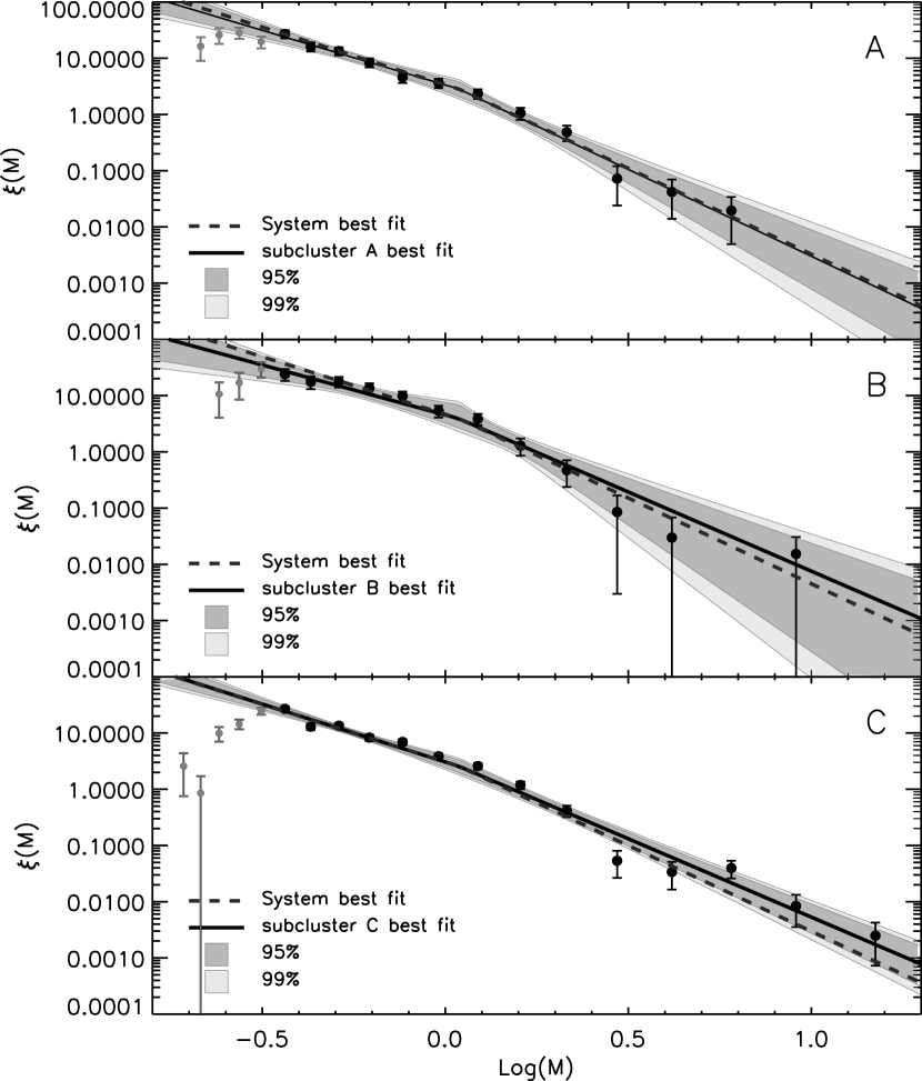
We applied the same method used in §5.1 and 5.2, isolating each time the regions of the sub-clusters, as shown in Figure 4b, iterating the Monte Carlo field subtraction, computing the distribution of number of stars in mass bins and correcting for incompleteness. For the model fitting, we used the same Levenberg-Marquard technique, with the difference that, in this case, we constrained the position of the break point between the two power-laws to be the same as for the general IMF, namely, at $\log(M/M_{\odot})=0.04$. This choice is reasonable considering that we are mainly interested in eventual changes in the derived slopes of the IMF.

The constructed IMF for each sub-cluster is shown in Figure 13. The overall IMF for the whole system is also overlayed, after it is normalized in order to match the subclusters’ best fit on the break point. In each case the IMF for the subsolar masses is the same as the general IMF, as discussed in §6 for the entire system of LH 95. Moreover, the derived two-phase models that fit the IMF of each sub-cluster and the corresponding uncertainties, given in Table 4, are compatible to that of the overall IMF given in Table 3.

Table 4IMF slopes and uncertainties for the three sub-clusters of LH 95

	$-0.5<\log(M/M_{\odot})<0.04$	$\log(M/M_{\odot})>0.04$
subcluster A	$0.94^{-0.40}_{+0.41}$	$2.09^{-0.55}_{+0.70}$
subcluster B	$0.78^{-0.77}_{+0.53}$	$1.82^{-0.60}_{+1.71}$
subcluster C	$1.05^{-0.35}_{+0.33}$	$1.79^{-0.29}_{+0.36}$

Note. — slopes are in terms of $x$ according to Equation 8, uncertainties are $95\%$ confidence intervals.

The IMF constructed for each sub-cluster in LH 95 suggests that the mass distribution of the PMS stars in this association does not vary much with location. Moreover, the spatial distribution of the intermediate- and high-mass stars within the whole of the system does not show any indication that the system is mass segregated. On the other hand if the individual sub-clusters are considered, the more massive stars do occupy the central parts of each of them, providing clear evidence that mass segregation in LH 95 probably occurs in rather small clustering scales.

According to recent results by Weidner & Kroupa (2006) on the integrated galaxial stellar IMF, the overall IMF of a composite system should be steeper than the one it would have if it was not composite, in the intermediate- and high-mass regime. Taking into account the fact that LH 95 is resolved into at least three individual subclusters (§3.2), it may be considered as a scaled-down case of the scenario of these authors, and therefore as a composite system. It should be noted that also this may explain the somewhat steep slope of the IMF we derive for LH 95.

7. Conclusions

We present a comprehensive investigation of the stellar populations of the star-forming association LH 95, located on the north-western edge of the super-giant shell LMC 4 in the Large Magellanic Cloud, using of deep HST/ACS photometry in the filters $F555W$ and $F814W$ (proxies for standard $V$ and $I$ respectively). Our findings can be summarized as follows.

We construct a new set of observational PMS models (both isochrones and evolutionary tracks) by starting from the original computations by Siess et al. (2000) and performing synthetic photometry on artificial stellar spectra. The latter were derived from interpolation of atmosphere models from the NextGen (Hauschildt et al., 1999) and Kurucz (Kurucz, 1993) grids. This approach enabled several improvements considering observed data for PMS stars. Specifically:

• We computed absolute magnitudes for each point of the original theoretical models in 88 different photometric bands, including the ACS/WFC system, which is useful for our observations. The availability of observational PMS evolutionary models in any given photometric system allows us to avoid the application of any color corrections to the observed data, or to approximate observations in the ACS/WFC system with any standard photometric system.

• Our computations, being similar to that of Girardi et al. (2002), do not rely on a single dependence on effective temperature for the computation of colors and magnitudes, but they also take into account the dependencies on the stellar surface gravities (i.e. in luminosity), and therefore they provide a more accurate treatment of the young stages of PMS evolution.

• These observational models are extrapolated to lower metallicities than those of Siess et al. (2000) by computing our synthetic photometry for the average LMC and SMC metallicities of $Z=0.008$ and $Z=0.004$, respectively.

We enhanced the catalog of stars detected in the observed field around the association LH 95 with ACS (Gouliermis et al., 2007) by identifying new point sources, which were previously rejected by the photometry mostly in crowded regions. Therefore, about $900$ additional stars are included in our photometric catalog (Table 1), which now includes in total 17,245 stars. Our deep ACS photometry allowed us to analyze the properties of the abundant PMS population found in LH 95, which shows an average age of 4 Myr. We performed star counts on our stellar sample of the area of the association and we selected the central part of the observed field, where a statistically significant concentration of PMS stars is found, as the most representative region of LH 95. The 3$\sigma$ isopleth was selected to define the boundaries of the system. The PMS stars within the association are found to be mostly concentrated in three distinctive sub-clusters, named cluster A, B and C respective, providing evidence of the existence of stellar subgroups within a single association.

We estimate the total stellar masses and corresponding dynamical timescales for the system itself as well as the three subclusters, and we find that the system cannot be considered dynamically evolved, and it does not experience any disruption. Moreover, the fact that LH 95 is a bound cluster with its gas partially removed implies that the star formation efficiency is probably higher than the typical values for young clusters.

We estimated the stellar contribution of the general background field of the galaxy in the area of the system from our ACS observations of a nearby control field. We then performed field subtraction from the area of the system with the use of Monte Carlo simulations.

With our evolutionary models we estimated the interstellar extinction in LH 95 and we computed the masses of all the members of the system. Our stellar sample reaches masses as low as $\sim$ 0.2 M_⊙, and we are able to correct the incompleteness accurately down to $\simeq$ 0.43 M_⊙. For the first time, this allows the construction of the extragalactic IMF down to the sub-solar mass regime.

We derive the system IMF by counting stars within bins of variable width, which increase with mass, and correcting for incompleteness based on artificial star experiments for the stars included in each mass range. We derive the actual statistical distribution of the counting errors associated to each mass bin via a Monte Carlo technique, in order to take into account uncertainties introduced by the contamination from the field population. The statistical F test for model selection allowed us to determine a two-phase power-law as the most appropriate model to fit our IMF. We detect a change in the slope of the IMF (the “knee” of the IMF) for masses lower than 1 M_⊙. A Levenberg-Marquard algorithm for least square fitting was applied to determine the power-law exponents and the point where the slope changes. The derived system IMF slope is found to be $x=1.05^{-0.20}_{+0.15}$ in the subsolar regime, and $x=2.05^{-0.28}_{+0.39}$ at intermediate and high masses, with a $95\%$ of confidence.

This system IMF, once corrected for unresolved binarity, is statistically compatible, within the studied mass range, with the average Galactic IMF, concerning its slope and the mass limit where it changes (1 M_⊙). As a consequence, we cannot consider the metallicity difference between the LMC ($Z=0.008$) and the Galaxy important enough for a significant change in the IMF slope. Certainly similar data on such stellar systems will show if this is a normal behavior of the IMF in this galaxy. We find no significant differences in the shape of the overall IMF of LH 95 from that of each of the three individual PMS sub-clusters of the association. This clearly suggests that the IMF of LH 95 is not subject to local variability.

References

- Alcock et al. (2004) Alcock, C., et al. 2004, AJ, 127, 334
- Allen et al. (2007) Allen, L., et al. 2007, Protostars and Planets V, 361
- Ambartsumian (1947) Ambartsumian, V. A. 1947, In Stellar Evolution and Astrophysics, Armenian Acad. of Sci.
- Baraffe et al. (1998) Baraffe, I., Chabrier, G., Allard, F., & Hauschildt, P. H. 1998, A&A, 337, 403
- Baraffe et al. (2001) Baraffe, I., Chabrier, G., Allard, F., Hauschildt, P. 2001, From Darkness to Light: Origin and Evolution of Young Stellar Clusters, 243, 571
- Barrado y Navascués et al. (2001) Barrado y Navascués, D., Stauffer, J. R., Bouvier, J., & Martín, E. L. 2001, ApJ, 546, 1006
- Bohlin (2007) Bohlin, R. C. 2007, The Future of Photometric, Spectrophotometric and Polarimetric Standardization, 364, 315
- Bouchet et al. (1985) Bouchet, P., Lequeux, J., Maurice, E., Prevot, L., & Prevot-Burnichon, M. L. 1985, A&A, 149, 330
- Briceño et al. (2007) Briceño, C., Hartmann, L., Hernández, J., Calvet, N., Vivas, A. K., Furesz, G., & Szentgyorgyi, A. 2007, ApJ, 661, 1119
- Cardelli et al. (1989) Cardelli, J. A., Clayton, G. C., Mathis, J. S. 1989, ApJ, 345, 245
- Caldwell & Coulson (1986) Caldwell, J. A. R., & Coulson, I. M. 1986, MNRAS, 218, 223
- Cole (1998) Cole, A. A. 1998, ApJ, 500, L137
- Chabrier (2003) Chabrier, G. 2003, PASP, 115, 763
- D’Antona & Mazzitelli (1994) D’Antona, F., Mazzitelli, I. 1994, ApJS, 90, 467
- D’Antona & Mazzitelli (1997) D’Antona, F., Mazzitelli, I. 1997, Memorie della Societa Astronomica Italiana, 68, 807
- Dolphin & Hunter (1998) Dolphin, A. E., & Hunter, D. A. 1998, AJ, 116, 1275
- Dolphin (2000) Dolphin, A. E. 2000, PASP, 112, 1383
- Fellhauer et al. (2006) Fellhauer, M., Kroupa, P., & Evans, N. W. 2006, MNRAS, 372, 338
- Girardi et al. (2002) Girardi, L., Bertelli, G., Bressan, A., Chiosi, C., Groenewegen, M. A. T., Marigo, P., Salasnich, B., Weiss, A. 2002, A&A, 391, 195
- Gouliermis et al. (2002) Gouliermis, D., Keller, S. C., de Boer, K. S., Kontizas, M., & Kontizas, E. 2002, A&A, 381, 862
- Gouliermis et al. (2006a) Gouliermis, D., Brandner, W., & Henning, Th. 2006a, ApJ, 636, L133
- Gouliermis et al. (2006b) Gouliermis, D. A., Dolphin, A. E., Brandner, W., & Henning, Th. 2006b, ApJS, 166, 549
- Gouliermis et al. (2007) Gouliermis, D. A., Henning, Th., Brandner, W., Dolphin, A. E., Rosa, M., Brandl, B. 2007, ApJ, 665, L27 (Paper I)
- Hauschildt et al. (1999) Hauschildt, P. H., Allard, F., Ferguson, J., Baron, E., & Alexander, D. R. 1999, ApJ, 525, 871
- Hennekemper et al. (2008) Hennekemper, E., Gouliermis, D. A., Henning, Th., Brandner, W., & Dolphin, A. E. 2008, ApJ, 672, 914
- Hill et al. (1994) Hill, R. J., Madore, B. F., & Freedman, W. L. 1994, ApJ, 429, 204
- Hill et al. (1995) Hill, R. S., Cheng, K.-P., Bohlin, R. C., O’Connell, R. W., Roberts, M. S., Smith, A. M., & Stecher, T. P. 1995, ApJ, 446, 622
- Kenyon & Hartmann (1995) Kenyon, S. J., Hartmann, L. 1995, ApJS, 101, 117
- Kontizas et al. (1993) Kontizas, M., Kontizas, E., & Michalitsianos, A. G. 1993, A&A, 269, 107
- Koornneef (1982) Koornneef, J. 1982, A&A, 107, 247
- Kroupa et al. (1991) Kroupa, P., Gilmore, G., & Tout, C. A. 1991, MNRAS, 251, 293
- Kroupa et al. (1993) Kroupa, P., Tout, C. A., & Gilmore, G. 1993, MNRAS, 262, 545
- Kroupa (2001) Kroupa, P. 2001, MNRAS, 322, 231
- Kroupa (2002) Kroupa, P. 2002, Science, 295, 82
- Kroupa (2008) Kroupa, P. 2008, in The Cambridge N-body Lectures, S. Aarseth, C. Tout, R. Mardling (eds), Lecture Notes in Physics Series, Springer Verlag (arXiv:0803.1833)
- Kurucz (1979) Kurucz, R. 1979, ApJS, 40, 1
- Kurucz (1993) Kurucz, R. 1993, ATLAS9 Stellar Atmosphere Programs and 2 km/s grid. Kurucz CD-ROM No. 13. Cambridge, Mass.: Smithsonian Astrophysical Observatory, 1993., 13
- Lada & Lada (2003) Lada, C. J., & Lada, E. A. 2003, ARA&A, 41, 57
- Levenberg (1944) Levenberg, K. 1944, The Quarterly of Applied Mathematics 2, 164
- Luck et al. (1998) Luck, R. E., Moffett, T. J., Barnes, T. G., III, & Gieren, W. P. 1998, AJ, 115, 605
- Maíz-Apellániz (2004) Maíz-Apellániz, J. 2004, PASP, 116, 859
- Maíz-Apellániz & Úbeda (2005) Maíz Apellániz, J., & Úbeda, L. 2005, ApJ, 629, 873
- Maíz-Apellániz (2007) Maíz-Apellániz, J. 2007, The Future of Photometric, Spectrophotometric and Polarimetric Standardization, 364, 227
- Marks et al. (2008) Marks, M., Kroupa, P., & Baumgardt, H. 2008, MNRAS, 386, 2047
- Marquardt (1963) Marquardt, D. 1963, SIAM Journal on Applied Mathematics 11, 431
- Massey et al. (1989a) Massey, P., Silkey, M., Garmany, C. D., & Degioia-Eastwood, K. 1989a, AJ, 97, 107
- Massey et al. (1989b) Massey, P., Parker, J. W., & Garmany, C. D. 1989b, AJ, 98, 1305
- Massey et al. (1995) Massey, P., Lang, C. C., Degioia-Eastwood, K., & Garmany, C. D. 1995, ApJ, 438, 188
- Massey & Hunter (1998) Massey, P., & Hunter, D. A. 1998, ApJ, 493, 180
- Massey (2003) Massey, P. 2003, ARA&A, 41, 15
- Nota et al. (2006) Nota, A., et al. 2006, ApJ, 640, L29
- Oey (1996) Oey, M. S. 1996, ApJS, 104, 71
- Palla & Stahler (1999) Palla, F., Stahler, S. W. 1999, ApJ, 525, 772
- Palla & Stahler (2000) Palla, F., & Stahler, S. W. 2000, ApJ, 540, 255
- Pei et al. (1999) Pei, Y. C., Fall, S. M., & Hauser, M. G. 1999, ApJ, 522, 604
- Piotto & Zoccali (1999) Piotto, G., & Zoccali, M. 1999, A&A, 345, 485
- Preibisch et al. (2002) Preibisch, T., Brown, A. G. A., Bridges, T., Guenther, E., & Zinnecker, H. 2002, AJ, 124, 404
- Reylé & Robin (2001) Reylé, C., & Robin, A. C. 2001, A&A, 373, 886
- Sabbi et al. (2008) Sabbi, E., et al. 2008, AJ, 135, 173
- Sagar & Richtler (1991) Sagar, R., & Richtler, T. 1991, A&A, 250, 324
- Salpeter (1955) Salpeter, E. E. 1955, ApJ, 121, 161
- Scalo (1986) Scalo, J. M. 1986, Fundamentals of Cosmic Physics, 11, 1
- Scalo (1998) Scalo, J. 1998, The Stellar Initial Mass Function (38th Herstmonceux Conference), 142, 201
- Schmalzl et al. (2008) Schmalzl, M., Gouliermis, D. A., Dolphin, A. E., & Henning, Th. 2008, ApJ, 681, 290
- Sherry et al. (2004) Sherry, W. H., Walter, F. M., & Wolk, S. J. 2004, AJ, 128, 2316
- Siess et al. (1997) Siess, L., Forestini, M., Dougados, C. 1997, A&A, 324, 556
- Siess et al. (2000) Siess, L., Dufour, E., Forestini, M. 2000, A&A, 358, 593
- Spitzer (1958) Spitzer, L. Jr. 1958, ApJ, 127, 17
- Swenson et al. (1994) Swenson, F. J., Faulkner, J., Rogers, F. J., & Iglesias, C. A. 1994, ApJ, 425, 286
- Weidner & Kroupa (2006) Weidner, C., & Kroupa, P. 2006, MNRAS, 365, 1333
- Weidner et al. (2008) Weidner, C., Kroupa, P., & Maschberger, T. 2008, accepted for publication in MNRAS (arXiv:0811.3730)
- Westerlund (1997) Westerlund, B. E. 1997, The Magellanic Clouds (Cambridge: Cambridge Univ. Press)
- Wilking & Lada (1983) Wilking, B. A., & Lada, C. J. 1983, ApJ, 274, 698