Gene ranking and biomarker discovery under correlation

Abstract

Motivation: Biomarker discovery and gene ranking is a standard task in genomic high throughput analysis. Typically, the ordering of markers is based on a stabilized variant of the $t$-score, such as the moderated $t$ or the SAM statistic. However, these procedures ignore gene-gene correlations, which may have a profound impact on the gene orderings and on the power of the subsequent tests.

Results: We propose a simple procedure that adjusts gene-wise $t$-statistics to take account of correlations among genes. The resulting correlation-adjusted $t$-scores (“cat” scores) are derived from a predictive perspective, i.e. as a score for variable selection to discriminate group membership in two-class linear discriminant analysis. In the absence of correlation the cat score reduces to the standard $t$-score. Moreover, using the cat score it is straightforward to evaluate groups of features (i.e. gene sets). For computation of the cat score from small sample data we propose a shrinkage procedure. In a comparative study comprising six different synthetic and empirical correlation structures we show that the cat score improves estimation of gene orderings and leads to higher power for fixed true discovery rate, and vice versa. Finally, we also illustrate the cat score by analyzing metabolomic data.

Availability: The shrinkage cat score is implemented in the R package “st” available from URL http://cran.r-project.org/web/packages/st/.

Contact: strimmer@uni-leipzig.de

1 Introduction

The discovery of genomic biomarkers is often based on case-control studies. For instance, consider a typical microarray experiment comparing healthy to cancer tissue. A shortlist of genes relevant for discriminating the phenotype of interest is compiled by ranking genes according to their respective $t$-scores. Because of the high-dimensionality of the genomic data special stabilizing procedures such as “SAM”, “moderated $t$” or “shrinkage $t$” are warranted and most effective – see Opgen-Rhein and Strimmer, (2007) for a recent comparative study.

However, microarrays are only one particularly prominent example of a series of modern technologies emerging for high-throughput biomarker discovery. In addition to gene expression it is now common practice in biomedical laboratories to measure metabolite concentrations and protein abundances. A distinguishing feature of proteomic and metabolic data is the presence of correlation among markers, due to chemical similarities (metabolites) and spatial dependencies (spectral data). These correlations may impact statistical conclusions.

There are three main strategies for dealing with the issue of correlation among biomarkers. One approach is to initially ignore the correlation structure and to compute conventional $t$-scores. Subsequently, the effects of correlation are accommodated in the last stage of the analysis when statistical significance is assigned (Efron,, 2007; Shi et al.,, 2008). An alternative approach is to model the correlation structure explicitly in the data generating process, and base all inferences on this more complex model. For example, in case of proteomics data a spatial autoregressive model can account for dependencies between neighboring peaks (Hand,, 2008). A third strategy, occupying middle ground between the two described approaches, is to combine $t$-scores and the estimated correlations to a new gene-wise test statistic. This approach is followed in Tibshirani and Wasserman, (2006) and Lai, (2008) and it is also the route we pursue here.

Specifically, we propose “correlation-adjusted $t$”-scores, or short “cat” scores. These scores are derived from a predictive perspective by exploiting a close link between gene ranking and and two-class linear discriminant analysis (LDA). It is well known (Fan and Fan,, 2008) that the $t$-score is the natural feature selection criterion in diagonal discriminant analysis, i.e. when there is no correlation. As we argue here in the general LDA case assuming arbitrary correlation structure this role is taken over by the cat score.

For practical application of the cat score as a ranking criterion for biomarkers we develop a corresponding shrinkage procedure, which can be employed in high-dimensional settings with a comparatively small number of samples. This statistic reduces to the shrinkage $t$ approach (Opgen-Rhein and Strimmer,, 2007) if there is no correlation. We also provide a recipe for constructing cat scores from other regularized $t$-statistics. Furthermore, we show that the cat score enables in a straightforward fashion the ranking of sets of features and thus facilitates the analysis of gene set enrichment (Ackermann and Strimmer,, 2009).

The rest of the paper is organized as follows. Next, we present the methodological background, the definition of the cat score, and a corresponding small sample shrinkage procedure. Subsequently, we report results from a comparative study where we investigate the performance of the shrinkage cat score relative to other gene ranking procedures including the approaches by Tibshirani and Wasserman, (2006) and Lai, (2008). In our study we assume a variety of both synthetic as well as empirical correlation scenarios from gene expression data. Finally, we illustrate the cat score approach by analyzing a metabolomic data set and conclude with recommendations.

2 Methods

2.1 Linear discriminant analysis

Linear discriminant analysis (LDA) is a simple yet very effective classification algorithm (Hand,, 2006). If there are $K$ distinct class labels, then LDA assumes that each class can be represented by a multivariate normal density

$$\begin{split}f(\boldsymbol{x}|k)&=(2\pi)^{-p/2}|\boldsymbol{\Sigma}|^{-1/2}\;\times\\ &\mathrel{\phantom{=}}\exp\{-\frac{1}{2}(\boldsymbol{x}-\boldsymbol{\mu}_{k})^{T}\boldsymbol{\Sigma}^{-1}(\boldsymbol{x}-\boldsymbol{\mu}_{k})\}\end{split}$$

with mean $\boldsymbol{\mu}_{k}$ and a common covariance matrix $\boldsymbol{\Sigma}$, which can be decomposed into $\boldsymbol{\Sigma}=\boldsymbol{V}^{1/2}\boldsymbol{P}\boldsymbol{V}^{1/2}$ with correlations $\boldsymbol{P}=(\rho_{ij})$ and variances $\boldsymbol{V}=\text{diag}\{\sigma^{2}_{1},\ldots,\sigma^{2}_{p}\}$. The observed $p$-dimensional data $\boldsymbol{x}$ (e.g., the expression levels of all genes in a sample) are thus modeled by the mixture

$$f(\boldsymbol{x})=\sum_{j=1}^{K}\pi_{j}f(\boldsymbol{x}|j),$$

where the $\pi_{j}$ are the a priori mixing weights. Applying Bayes’ theorem gives the probability of group $k$ given $\boldsymbol{x}$,

$$\text{Pr}(k|\boldsymbol{x})=\frac{\pi_{k}f(\boldsymbol{x}|k)}{f(\boldsymbol{x})},$$

which in turns allows to define the discriminant score $d_{k}(\boldsymbol{x})=\log\{\text{Pr}(k|\boldsymbol{x})\}$. Dropping terms constant across groups this results for LDA in

$$\begin{split}d_{k}^{\text{LDA}}(\boldsymbol{x})&=\boldsymbol{\mu}_{k}^{T}\boldsymbol{\Sigma}^{-1}\boldsymbol{x}-\frac{1}{2}\boldsymbol{\mu}_{k}^{T}\boldsymbol{\Sigma}^{-1}\boldsymbol{\mu}_{k}+\log(\pi_{k})\\ &=\boldsymbol{\mu}_{k}^{T}(\boldsymbol{V}^{1/2}\boldsymbol{P}\boldsymbol{V}^{1/2})^{-1}\boldsymbol{x}\\ &\phantom{=}-\frac{1}{2}\boldsymbol{\mu}_{k}^{T}(\boldsymbol{V}^{1/2}\boldsymbol{P}\boldsymbol{V}^{1/2})^{-1}\boldsymbol{\mu}_{k}+\log(\pi_{k})\,.\end{split}$$

Due to the common covariance $d_{k}^{\text{LDA}}(\boldsymbol{x})$ is linear in $\boldsymbol{x}$, hence the name of the procedure. In order to assign a class label to a data sample $\boldsymbol{x}$ the discriminant function for all classes is computed, and the class is selected that maximizes $d_{k}(\boldsymbol{x})$. The discriminant function itself is learned from a separate training data set (i.e. independently from the test samples).

An important special case of LDA is diagonal discriminant analysis (DDA), to which LDA reduces if there is no correlation ($\boldsymbol{P}=\boldsymbol{I}$) among features. Then the discriminant function simplifies to

$$d_{k}^{\text{DDA}}(\boldsymbol{x})=\boldsymbol{\mu}_{k}^{T}\boldsymbol{V}^{-1}\boldsymbol{x}-\frac{1}{2}\boldsymbol{\mu}_{k}^{T}\boldsymbol{V}^{-1}\boldsymbol{\mu}_{k}+\log(\pi_{k}).$$

In the machine learning literature prediction using the function $d_{k}^{\text{DDA}}(\boldsymbol{x})$ is known as “naive Bayes” classification (Bickel and Levina,, 2004).

2.2 Feature selection in two-class LDA

Gene ranking and feature selection for class prediction are closely connected. We exploit this here to define a score for ranking genes (features) in the presence of correlation. In what follows, we consider LDA for precisely two classes, i.e. the typical setup in case-control studies.

For $K=2$ the difference $\Delta^{\text{LDA}}(\boldsymbol{x})=d_{1}^{\text{LDA}}(\boldsymbol{x})-d_{2}^{\text{LDA}}(\boldsymbol{x})$ between the discriminant scores of the two classes provides a simple prediction rule: if $\Delta^{\text{LDA}}\geq 0$ then a test sample is assigned to class 1, otherwise class 2 is chosen. $\Delta^{\text{LDA}}(\boldsymbol{x})$ can be written after some algebra

$$\Delta^{\text{LDA}}(\boldsymbol{x})=\boldsymbol{\omega}^{T}\boldsymbol{\delta}(\boldsymbol{x})+\log(\frac{\pi_{1}}{\pi_{2}})$$ (1)

with weight vector

$$\boldsymbol{\omega}=\boldsymbol{P}^{-1/2}\boldsymbol{V}^{-1/2}(\boldsymbol{\mu}_{1}-\boldsymbol{\mu}_{2})$$ (2)

and vector-valued distance function

$$\boldsymbol{\delta}(\boldsymbol{x})=\boldsymbol{P}^{-1/2}\boldsymbol{V}^{-1/2}(\boldsymbol{x}-\frac{\boldsymbol{\mu}_{1}+\boldsymbol{\mu}_{2}}{2}).$$ (3)

The benefit of expressing two-class LDA in this fashion is that it clarifies the underlying mechanism. In particular, the difference score $\Delta^{\text{LDA}}(\boldsymbol{x})$ is governed solely by three factors:

• the log-ratio of the mixing proportions $\pi_{1}$ and $\pi_{2}$,

• $\boldsymbol{\delta}(\boldsymbol{x})$, the standardized and decorrelated distance of the test sample $\boldsymbol{x}$ to the average centroid, and

• the variable-specific feature weights $\boldsymbol{\omega}$.

Note in particular that the weight vector $\boldsymbol{\omega}$ is not a function of the test data $\boldsymbol{x}$ and that it carries no units of measurements. Its components $\omega_{i}$ directly control how much each particular gene $i$ contributes to the overall score $\Delta^{\text{LDA}}$. Thus, $\boldsymbol{\omega}$ is a natural univariate indicator for feature selection in two-class linear discriminant analysis. Moreover, note that the function $\boldsymbol{\delta}(\boldsymbol{x})$ is a Mahalanobis transform, i.e. the predictors $\boldsymbol{x}$ are centered, standardized and sphered before feature selection.

The interpretation of $\boldsymbol{\omega}$ as general feature weights is supported by considering the special case of DDA. In the absence of correlation the weights $\boldsymbol{\omega}$ directly reduce to $\boldsymbol{V}^{-1/2}(\boldsymbol{\mu}_{1}-\boldsymbol{\mu}_{2})$, which is (apart from a constant) the usual vector of two-sample $t$-scores. It is well known that in the DDA setting the $t$-score is the natural and optimal ranking criterion for discovering genes that best differentiate the two classes (Fan and Fan,, 2008). Note that if we would (hypothetically) decompose the product $\boldsymbol{\omega}^{T}\boldsymbol{\delta}(\boldsymbol{x})$ from Eq. 1 in a different fashion, e.g., such that the factor $\boldsymbol{P}^{-1/2}\boldsymbol{V}^{-1/2}$ was moved from Eq. 3 to Eq. 2, then in the limit of vanishing correlation the ranking criterion would not be a $t$-score but rather $\boldsymbol{V}^{-1}(\boldsymbol{\mu}_{1}-\boldsymbol{\mu}_{2})$. Similarly, if we would move only the factor $\boldsymbol{P}^{-1/2}$ from Eq. 3 to Eq. 2, then a number of other inconsistencies arise, in particular the connection of $\boldsymbol{\omega}$ with Hotelling’s $T^{2}$ statistic (see further below) is lost. Therefore, the decomposition as given by Eq. 2 and Eq. 3 is the most natural.

2.3 Definition of the correlation-adjusted $t$-score (cat score)

Figure 1: Relationship between fold change, $t$-score, and the cat score. The constant $c$ equals $(\frac{1}{n_{1}}+\frac{1}{n_{2}})^{-1/2}$.

Using the above we define the vector $\boldsymbol{\tau}^{adj}$ of “correlation-adjusted $t$-scores” (“cat score”) to be proportional to the feature weight vector $\boldsymbol{\omega}$ (Eq. 2):

$$\begin{split}\boldsymbol{\tau}^{adj}&\equiv(\frac{1}{n_{1}}+\frac{1}{n_{2}})^{-1/2}\,\boldsymbol{\omega}\\ &=\boldsymbol{P}^{-1/2}\times\{(\frac{1}{n_{1}}+\frac{1}{n_{2}})\boldsymbol{V}\}^{-1/2}(\boldsymbol{\mu}_{1}-\boldsymbol{\mu}_{2})\\ &=\boldsymbol{P}^{-1/2}\boldsymbol{\tau}.\end{split}$$ (4)

Note the scale factor $(\frac{1}{n_{1}}+\frac{1}{n_{2}})^{-1/2}$ ensures that the empirical version of the cat score matches the scale of the empirical $t$-score. The vector $\boldsymbol{\tau}$ contains the gene-wise $t$-scores, and $n_{k}$ is the number of observations in group $k$.

The cat score is a natural and intuitive extension of both the fold change and $t$-score, as illustrated in Fig. 1. While the $t$-score is the standardized mean difference $\boldsymbol{\mu}_{1}-\boldsymbol{\mu}_{2}$, the cat score is the standardized as well as decorrelated mean difference. The factor $\boldsymbol{P}^{-1/2}$ responsible for the decorrelation is well-known from the Mahalanobis transform that is frequently applied to prewhiten multivariate data. Also note that the inverse correlation matrix is closely related to partial correlations.

2.4 Estimation of feature weights and computation of the cat score from data

Substituting empirical estimates for means, variances, and correlations into Eqs. 2 and 4 provides a simple recipe for estimating the feature weights and computing the cat score from data. However, this is only a valid approach if sample size is large compared to the dimension.

For small-sample yet high-dimensional settings we suggest to employ James-Stein-type shrinkage estimators of correlation (Schäfer and Strimmer,, 2005) and of variances (Opgen-Rhein and Strimmer,, 2007). Plugging these two James-Stein-type estimators into Eq. 4 yields a shrinkage version of the cat score

$$\boldsymbol{t}^{\text{adj}}_{\text{shrink}}=(\boldsymbol{R}^{\text{shrink}})^{-1/2}\;\boldsymbol{t}^{\text{shrink}}.$$ (5)

A major obstacle in the application of Eq. 5 is the problem of efficiently computing $(\boldsymbol{R}^{\text{shrink}})^{-1/2}$. Direct calculation of the matrix square root, e.g., by eigenvalue decomposition, is extremely tedious for large dimensions $p$. Instead, we present here a simple time-saving identity for computing the $\alpha$-th power of $\boldsymbol{R}^{\text{shrink}}$ (though here we only need the case $\alpha=-1/2$).

The shrinkage correlation estimator of Schäfer and Strimmer, (2005) is given by $\boldsymbol{R}^{\text{shrink}}=\gamma\boldsymbol{I}_{p}+(1-\gamma)\boldsymbol{R}$, where $\boldsymbol{R}$ is the empirical correlation matrix and $\gamma$ the shrinkage intensity. We define $\boldsymbol{Z}=\boldsymbol{R}^{\text{shrink}}/\gamma=\boldsymbol{I}_{p}+\frac{1-\gamma}{\gamma}\boldsymbol{R}=\boldsymbol{I}_{p}+\boldsymbol{U}\boldsymbol{M}\boldsymbol{U}^{T}$, where $\boldsymbol{M}$ is a symmetric positive definite matrix of size $m$ times $m$ and $\boldsymbol{U}$ an orthonormal basis. Note that $m$ is the rank of $\boldsymbol{R}$. Subsequently, to calculate the $\alpha$-th power of $\boldsymbol{Z}$ we use the identity

$$\boldsymbol{Z}^{\alpha}=\boldsymbol{I}_{p}-\boldsymbol{U}(\boldsymbol{I}_{m}-(\boldsymbol{I}_{m}+\boldsymbol{M})^{\alpha})\boldsymbol{U}^{T}$$ (6)

that requires only the computation of the $\alpha$-th power of the matrix $\boldsymbol{I}_{m}+\boldsymbol{M}$. This trick enables substantial computational savings when the number of samples (and hence $m$) is much smaller than $p$.

We note that identity Eq. 6 is related but not identical to the well-known Woodbury matrix identity for the inversion of a matrix. For $\alpha=-1$ our identity reduces to

$$\boldsymbol{Z}^{-1}=\boldsymbol{I}_{p}-\boldsymbol{U}(\boldsymbol{I}_{m}-(\boldsymbol{I}_{m}+\boldsymbol{M})^{-1})\boldsymbol{U}^{T},$$

whereas the Woodbury matrix identity equals

$$\boldsymbol{Z}^{-1}=\boldsymbol{I}_{p}-\boldsymbol{U}(\boldsymbol{I}_{m}+\boldsymbol{M}^{-1})^{-1}\boldsymbol{U}^{T}.$$

Finally, additional information about the structure of the correlation matrix $\boldsymbol{P}$ (or its inverse) may also be taken into account when estimating the cat score. This is done simply by replacing the unrestricted shrinkage estimator by a more structured estimator (e.g., Tai and Pan,, 2007; Li and Li,, 2008; Guillemot et al.,, 2008).

2.5 Selection of single genes

The cat score offers a simple approach to feature selection, both of individual genes and of sets of genes (see below).

By construction, the cat score is a decorrelated $t$-score. As such it measures the individual contribution of each single feature to separate the two groups, after removing the effect of all other genes. Therefore, to select individual genes according to their relative effect on group separation one simply ranks them according to the magnitude of the respective $\tau^{\text{adj}}_{i}$.

For determining $p$-values and FDR values we fit a two-component mixture model to the observed cat scores (Efron,, 2008). Asymptotically, for large dimension the null distribution is approximately normal as a consequence of central limit theorems for dependent random variables (e.g., Hoeffding and Robbins,, 1948; Romano and Wolf,, 2000) – recall that the cat score is a weighted sum over $p$ dependent $t$-statistics. This is validated empirically in section 3.5 discussing the analysis of a metabolomic data set.

For practical analysis we suggest employing the “fdrtool” algorithm (Strimmer, 2008a, ; Strimmer, 2008b, ). A comparison of methods for assigning significance to cat scores is given in Ahdesmäki and Strimmer, (2009).

2.6 Selection of gene sets

For evaluating the total effect of a set of features on group separation we exploit the close connection of cat scores with the Hotelling’s $T^{2}$ statistic, a standard criterion in gene set analysis (Lu et al.,, 2005; Kong et al.,, 2006).

Specifically, $T^{2}=(\boldsymbol{t}^{\text{adj}})^{T}\boldsymbol{t}^{\text{adj}}=\boldsymbol{t}^{T}\boldsymbol{R}^{-1}\boldsymbol{t}$, where $\boldsymbol{R}$ is the empirical correlation matrix, $\boldsymbol{t}^{\text{adj}}$ the empirical cat score vector, and $\boldsymbol{t}$ the vector containing the gene-wise Student $t$-statistic. In other words, the $T^{2}$ statistic is identical to the sum of the squared individual empirical cat scores for the genes in the set. Note that any normalization with regard to the size of the set is implicit in the factor $\boldsymbol{R}^{-1}$. For example, if there is strong correlation among the genes in a set then $T^{2}$ is approximately the average of the underlying squared $t$-scores.

With this in mind, we define the grouped cat score for gene $i$ belonging to a given gene set as the signed square root of the sum over the squared cat scores of all genes in the given gene set,

$$\tau^{\text{adj,grouped}}_{i}=\text{sign}(\tau^{\text{adj}}_{i})\sqrt{\sum_{g\in\text{gene set}}(\tau^{\text{adj}}_{g})^{2}}\,.$$

There are two main cases when it is important to consider sets of genes rather than individual genes:

• First, in a gene set enrichment analysis where prespecified pathways or functional units rather than individual genes are being investigated (cf. Ackermann and Strimmer, (2009)).

• Second, if genes are highly correlated and thus provide the same information on group separation. To accommodate for this collinearity we suggest constructing a suitable correlation neighborhood around each gene, e.g., by the rule $|r|\geq 0.85$. Typically, the resulting sets are rather small and for most genes are comprised only of the gene itself – see Tibshirani and Wasserman, (2006) and also Läuter et al., (2009) for similar procedures. Note that the suggested threshold of $0.85$ – which we use throughout this paper – is rather conservative. It defines a priori which pair of genes are assumed to be collinear.

We note that using the grouped cat score provides to a simple procedure for high-dimensional feature selection where whole sets of variables are simultaneously included or excluded, in contrast to the classical view of feature selection where only one of those features is retained (see also Bondell and Reich, (2008) for references to related approaches).

3 Results

In order to study the performance of the cat score for feature selection and gene ranking, we conducted an extensive study. Specifically, we investigated six different correlation scenarios, three synthetic models and three empirical correlation matrices estimated from three different gene expression data sets, and compared the results with a diverse number of regularized $t$-scores. Furthermore, we analyzed a metabolomic data set investigating prostate cancer.

3.1 Correlation scenarios

Figure 2: The six correlation scenarios investigated in our study. All correlation matrices have size $1000\times 1000$ and thus contain 499500 correlation values. Top row: Histograms of the correlations of three synthetic correlation patterns (A–C). Bottom row: Histograms of the three empirical correlation structures (D–F). For further details see main text.

For the correlation structure, we considered a variety of scenarios. Specifically, we employed six different correlation patterns (cf. Fig. 2):

• First, as a negative control we assumed a diagonal correlation matrix $\boldsymbol{P}=\boldsymbol{I}$ of size $1000\times 1000$.

• Next, we employed an autoregressive block-diagonal correlation matrix (Guo et al.,, 2007). We used 10 blocks of size $100\times 100$ genes. Within each block, the correlation between two genes $i,j,=1,\dots,100$ equals $\rho(i,j)=\rho^{\text{abs}(i-j)}$. We set $\rho=0.99$ with alternating sign in each block. This correlation matrix is sparse with most entries being very small, nevertheless it also contains some highly correlated genes.

• Third, we employed a correlation block structure where the first 100 genes have pairwise correlation of 0.7 and the remaining 900 genes have pairwise correlation of 0.3. Between the two groups there is no correlation. The block with the larger correlation corresponds to the differentially expressed genes.

• In addition to the three artificial correlation structures, we also employed shrinkage estimators of correlations matrices from three expression data sets, using a sample of 1000 genes. Structure D is obtained from gene expression data of colon cancer (Alon et al.,, 1999).

• As D, but for breast cancer (Hedenfalk et al.,, 2001).

• As D, but from a spike-in experiment (Choe et al.,, 2005).

3.2 Test statistics

In our comparison we included the following gene ranking statistics: fold change, empirical $t$ statistic, “SAM” (Tusher et al.,, 2001), “moderated $t$” Smyth, (2004), and “shrinkage $t$” Opgen-Rhein and Strimmer, (2007). As in Opgen-Rhein and Strimmer, (2007) the latter three regularized $t$-scores gave nearly identical estimates and always outperformed Student $t$, so we report here only the results for “shrinkage $t$”. As baseline reference we also included random ordering in the analysis.

For the cat score we investigated two variants: the shrinkage cat score (Eq. 5) and an oracle version, which uses the true underlying correlation matrix rather than estimating the correlation structure. For the two structures with high correlations (B and C) we employed the grouped cat score using a correlation neighborhood threshold of 0.85.

In addition, we included in our study two recently proposed gene ranking procedures that, like the cat score, also aim at incorporating information about gene-gene correlations in gene ranking: the “correlation-shared $t$-score” introduced by Tibshirani and Wasserman, (2006) and the “correlation-predicted $t$-score” suggested by Lai, (2008). Correlation-shared $t$ averages over gene-specific Student $t$-scores in a data-dependent correlation neighborhood. The approach by Lai, (2008) employs a local smoothing approach to “predict” the $t$-score of a particular gene from $t$-scores of other genes highly correlated with it. Here, we use the Lai, (2008) approach with the smoothing parameter set to its default value $f=0.2$. Note that the cat score, the correlation-shared $t$-score and the correlation-predicted $t$-score all are based on linear combinations of $t$-scores, albeit with different weights.

3.3 Data generation

In our data generation procedure we followed closely the setup in Smyth, (2004) and Opgen-Rhein and Strimmer, (2007), with the additional specification of a correlation structure among genes. In detail, the simulations were conducted as follows:

• The number of genes was fixed at $p=1000$. The first 100 genes were designated to be differentially expressed.

• The variances across genes were drawn from a scale-inverse-chi-square distribution $\text{Scale-inv-}\chi^{2}(d_{0},s_{0}^{2})$. We used $s^{2}_{0}=4$ and $d_{0}=4$, which corresponds to the “balanced” variance case in Smyth, (2004). Thus, the variances vary moderately from gene to gene.

• The difference of means for the differentially expressed genes (1–100) were drawn from a normal distribution with mean zero and the gene-specific variance. For the non-differentially expressed genes (101–1000) the difference was set to zero.

• The data were generated by drawing from group-specific multivariate normal distributions with the given variances and means. The correlation matrix assumed one of the above structures A–F.

• We also varied the sample sizes $n_{1}$ and $n_{2}$ in each group, from very small $n_{1}=n_{2}=3$ to fairly large $n_{1}=n_{2}=50$. Here, we report results for $n_{1}=n_{2}=8$.

3.4 Comparison of gene rankings

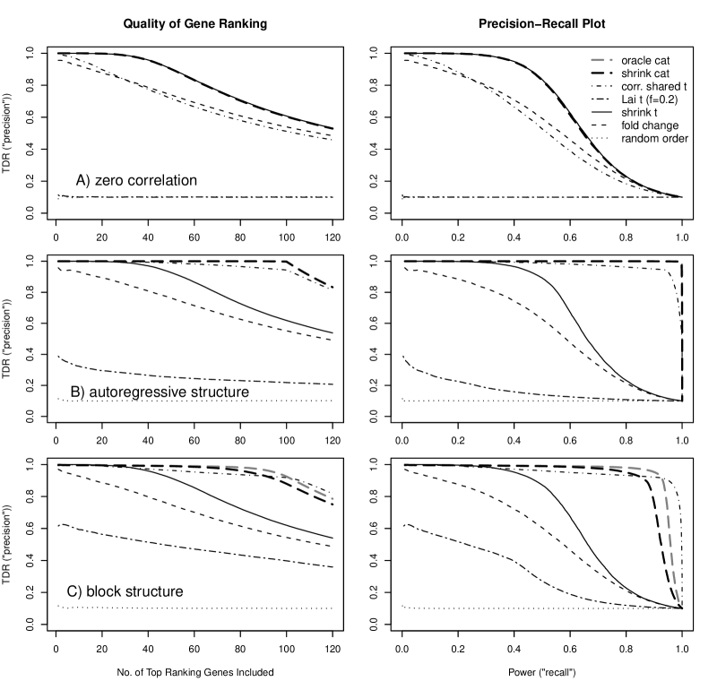
Figure 3: True discovery rates (left column) and precision-recall curves (right column) for the three synthetic correlation structures A–C. Note that for B and C the grouped cat score was employed, using a correlation neighborhood $|r|\geq 0.85$.

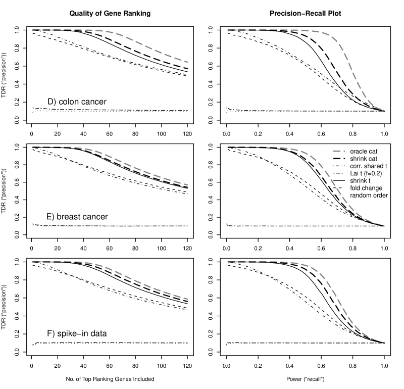
Figure 4: True discovery rates (left column) and precision-recall curves (right column) for the three empirical correlation scenarios D–F.

For each correlation scenario A–F we generated 500 data sets and computed corresponding gene rankings using the various $t$-scores and cat scores discussed above. We then counted false positives ($FP$), true positives ($TP$), false negatives ($FN$), and true negatives ($TN$) for all possible cut-offs in the gene list (1-1000). From this data we estimated the true discovery rates (= positive predictive value, ppv) $E(\frac{TP}{TP+FP})$ and the power (= sensitivity) $E(\frac{TP}{TP+FN})$.

A graphical summary of the results are presented in Fig. 3 and Fig. 4. The first column shows the true discovery rates as a function of the number of included top-ranking genes, whereas the second column gives the plots of true discovery rate versus power. The latter graphs, known in the machine learning community as “precision-recall” plots, highlight methods that simultaneously have large power and large true discovery rates.

The first row in Fig. 3 shows the control case when there is no correlation present. As expected, the cat score performs identical to the shrinkage $t$ approach. A similar performance is given by the correlation-shared $t$ and the fold change statistic, slightly worse than shrinkage $t$- and cat score. The ordering provided by the correlation-predicted $t$-score is random, which is not surprising as prediction fails when there is no correlation.

For the autoregressive and the block structure (scenarios B and C in Fig. 3) substantial gains are achieved over the shrinkage $t$-score, both by the cat score and the correlation-shared $t$-score by Tibshirani and Wasserman, (2006). In particular in case B these two methods show near-perfect recovery of the gene ranking. The shrinkage $t$ approach and fold change remain the second and third best feature ranking approach, with the correlation-predicted $t$-score of Lai, (2008) trailing the comparison.

For the empirically estimated correlation structures the picture changes slightly (cf. Fig. 4). All these scenarios have in common that there is common background correlation but no very strong individual pairwise correlations exist (cf. Fig. 2, bottom row). In this setting the shrinkage cat score also improves over the shrinkage $t$-score. The oracle cat score shows that further benefits are possible if the correlation structure was known, or if a better estimator was used. For the empirical scenarios the correlation-shared $t$-score performs similar as the fold change, and the correlation-predicted $t$-score again delivers random orderings.

In summary, in all the six quite different correlation scenarios the (grouped) cat score offers in part substantial performance improvements over standard regularized $t$-scores, which were represented here by shrinkage $t$-score. The correlation-shared $t$-score also performs exceptionally well if there are a few highly correlated genes, but otherwise falls back to the efficiency of using fold-change approach. The correlation-predicted approach did in general not provide any reasonable orderings. It seems to us that this is due to the fact that it is the only test statistic that discards the actual value of the $t$-score of a gene, and instead relies exclusively on closely correlated genes – which may not exist.

3.5 Ranking of metabolomic markers of prostate cancer

Figure 5: Plot of normal versus empirical quantiles for the grouped cat scores computed from the metabolomic prostate data. The linearity in the central part indicates a normal null model.

To illustrate the effect of correlation on gene ranking we analyzed a subset of data from a recent metabolomic study concerning prostate cancer (Sreekumar et al.,, 2009). The original study investigated three groups of tissues, benign, localized cancer and metastatic prostate cancer. Here, we focused on the two types of cancer tissue. Specifically, we compared 12 samples of clinically localized prostate cancers versus 14 samples of metastatic prostate cancers. For each sample the concentrations of 518 metabolites were measured. We use here the preprocessed data as kindly provided by Dr. Sreekumar and Dr. Chinnaiyan.

For each of the 518 metabolites we computed a shrinkage $t$-score and a shrinkage cat score. For the latter we applied grouping of features with a correlation threshold of $|r|\geq 0.85$. The Q-Q-plot of the cat scores versus a normal distribution is shown in Fig. 5. By inspection of this diagnostic plot we see that the null model of the grouped cat scores, represented by the linear middle part, is approximately a normal distribution. The deviations from normality at the tails correspond to the alternative distribution containing the high-ranked metabolites of interest.

Table 1: The top 10 ranking metabolites according to the shrinkage $t$ and the grouped cat scores, respectively. Note that nicotinamide and X-5207, as well as guanosine and X-3390, are strongly correlated.

Rank	shrinkage $t$	grouped cat score
1	Ciliatine	Nicotinamide
2	Inosine	X-5207
3	Putrescine	Guanosine
4	X-3390	X-3390
5	Palmitate	Ciliatine
6	Glycerol	Putrescine
7	Ribose	Inosine
8	X-3102	Citrate
9	Myristate	Uridine
10	X-4620	X-2867

The ten top ranking metabolic features that differentiate between localized and metastatic cancer according to $t$-scores and cat scores, respectively, are listed in Tab. 1. Overall, the two rankings differ quite notably, as expected in the presence of correlation. In particular, at the top of the list there are differences due to very strong correlation between the substrate X-5207 and Nicotinamide ($r=0.9444$) and likewise between Guanosine and X-3390 ($r=0.9389$). Unlike with $t$-scores, in a grouped cat score analysis the features in these two pairs are treated as a unit. Jointly, the correlated markers outperform other individual markers with respect to distinguishing between the two phenotypic groups.

Regarding the interpretation of observed enrichment of nicotinamide and guanosine, we caution that without further additional information it is not possible to decide whether this is due to intake of medication or rather due to the different progression of cancer.

For a series of other data examples further illustrating the analysis of cat scores and estimation of corresponding predictive errors we refer to Ahdesmäki and Strimmer, (2009).

4 Discussion

4.1 Harmonizing gene ranking and feature selection

The correlation-adjusted $t$-score is the result of our attempt to harmonize gene ranking with LDA feature selection. While it is well known that in the absence of correlation the $t$-score provides optimal rankings (Fan and Fan,, 2008), the situation is less clear in the LDA case where genes are allowed to be correlated. Here we show that the cat score provides a natural weight for feature selection in LDA analysis and that it can be sucessfully employed to rank genes and gene groups.

In order to apply cat scores in the analysis of high-dimensional data we develop in this paper a corresponding shrinkage procedure. For moderately high dimensions and sufficient sample size we demonstrate that incorporating correlation information into the gene ranking can lead to substantial improvement in power. However, this is only feasible if either the sample size is large or the signal is strong enough to estimate correlations (Hall et al.,, 2005). For microarray data with very small sample size (in the order of $n_{1}=n_{2}=3$) it is impossible to estimate a large-scale correlation matrix, and unsurprisingly for that case we did not see any benefits. However, as our study shows (Fig. 3 and Fig. 4) using the cat score can lead to substantial gains already for relatively moderate sample sizes ($n_{1}=n_{2}=8$).

4.2 Recommendations

In high-dimensional genomic experiments with very small sample size, when nothing is known a priori about the correlation structure, we recommend employing the standard regularized $t$-scores.

However, for moderate ratios of $p/n$, say smaller than 100, it is often possible to obtain reliable estimates of the correlation among markers. Thus, in this setting we propose ranking of biomarkers by the correlation-adjusted $t$-score, computed by the shrinkage procedure outlined above. In addition, if inspection of the correlation histogram shows existence of highly correlated features, then joint evaluation of those features by computing the grouped cat score is advised. Using more constrained correlation estimators may further improve the efficiency.

Finally, as pointed out by a referee, gene ranking by cat scores may be combined with fold change-based thresholding, in order to filter out statistically significant yet biologically irrelevant features (e.g. McCarthy and Smyth,, 2009).

In short, we propose to view gene ranking as a generically multivariate problem. In this perspective it seems stringent not only to standardize the mean differences (i.e. using the corresponding $t$-scores) but also to additionally decorrelate them, which results in the cat score proposed here.

Appendix: Computer implementation

The “shrinkage cat” estimator (Eq. 5) is implemented in the R package “st”, which is freely available under the terms of the GNU General Public License (version 3 or later) from CRAN (http://cran.r-project.org/) and from URL http://strimmerlab.org/software/st/.

References

- Ackermann and Strimmer, (2009) Ackermann, M. and Strimmer, K. (2009). A general modular framework for gene set enrichment. BMC Bioinformatics, 10:47.
- Ahdesmäki and Strimmer, (2009) Ahdesmäki, M. and Strimmer, K. (2009). Feature selection in “omics” prediction problems using cat scores and false non-discovery rate control. arXiv, stat.AP:0903.2003.
- Alon et al., (1999) Alon, U., Barkai, N., Notterman, D. A., Gish, K., Ybarra, S., Mack, D., and Levine, A. (1999). Broad patterns of gene expression revealed by clustering analysis of tumor and normal colon tissues probed by oligonucleotide arrays. Proc. Natl. Acad. Sci. USA, 96:6745–6750.
- Bickel and Levina, (2004) Bickel, P. J. and Levina, E. (2004). Some theory for Fisher’s linear discriminant function, ‘naive Bayes’, and some alternatives when there are many more variables than observations. Bernoulli, 10:989–1010.
- Bondell and Reich, (2008) Bondell, H. D. and Reich, B. J. (2008). Simultaneous regression shrinkage, variable selection, and supervised clustering of predictors with OSCAR. Biometrics, 64:115–123.
- Choe et al., (2005) Choe, S. E., Boutros, M., Michelson, A. M., Church, G. M., and Halfon, M. S. (2005). Preferred analysis methods for Affymetrix GeneChips revealed by a wholly defined control data set. Genome Biology, 6:R16.
- Efron, (2007) Efron, B. (2007). Correlation and large-scale simultaneous significance testing. J. Amer. Statist. Assoc., 102:93–103.
- Efron, (2008) Efron, B. (2008). Microarrays, empirical Bayes, and the two-groups model. Statist. Sci., 23:1–22.
- Fan and Fan, (2008) Fan, J. and Fan, Y. (2008). High-dimensional classification using features annealed independence rules. Ann. Statist., 36:2605–2637.
- Guillemot et al., (2008) Guillemot, V., Le Brusquet, L., Tenenhaus, A., and Frouin, V. (2008). Graph-constrained discriminant analysis of functional genomics data. In IEEE International Conference on Bioinformatics and Biomedicine, Philadelphia, PA, USA.
- Guo et al., (2007) Guo, Y., Hastie, T., and Tibshirani, T. (2007). Regularized discriminant analysis and its application in microarrays. Biostatistics, 8:86–100.
- Hall et al., (2005) Hall, P., Marron, J. S., and Neeman, A. (2005). Geometric representation of high dimension, low sample size data. J. R. Statist. Soc. B, 67:427–444.
- Hand, (2006) Hand, D. J. (2006). Classifier technology and the illusion of progress. Statistical Science, 21:1–14.
- Hand, (2008) Hand, D. J. (2008). Breast cancer diagnosis from proteomic mass spectrometry data: a comparative evaluation. Statist. Appl. Genet. Mol. Biol., 7 Issue 2:15.
- Hedenfalk et al., (2001) Hedenfalk, I., Duggan, D., Chen, Y., Radmacher, M., Bittner, M., Simon, R., Meltzer, P., Gusterson, B., Esteller, M., Kallioniemi, O. P., Wilfond, B., Borg, A., and Trent, J. (2001). Gene-expression profiles in hereditary breast cancer. N. Engl. J. Med., 344:539–548.
- Hoeffding and Robbins, (1948) Hoeffding, W. and Robbins, H. (1948). The central limit theorem for dependent random variables. Duke Math. J., 15:773–780.
- Kong et al., (2006) Kong, S. W., Pu, W. T., and Park, P. J. (2006). A multivariate approach for integrating genome-wide expression data and biological knowledge. Bioinformatics, 22:2373–2380.
- Lai, (2008) Lai, Y. (2008). Genome-wide co-expression based prediction of differential expression. Bioinformatics, 24:666–674.
- Läuter et al., (2009) Läuter, J., Horn, F., Rosolowski, M., and Glimm, E. (2009). High-dimensional data analysis: selection of variables, data compression and graphics — applications to gene expression. Biometr. J., 51:235–251.
- Li and Li, (2008) Li, C. and Li, H. (2008). Network-constrained regularization and variable selection for analysis of genomic data. Bioinformatics, 24:1175–1182.
- Lu et al., (2005) Lu, Y., Liu, P.-Y., Xiao, P., and Deng, H.-W. (2005). Hotelling’s multivariate profiling for detecting differential expression in microarrays. Bioinformatics, 21:3105–3113.
- McCarthy and Smyth, (2009) McCarthy, D. J. and Smyth, G. K. (2009). Testing significance relative to fold-change threshold is a TREAT. Bioinformatics, 25:765–771.
- Opgen-Rhein and Strimmer, (2007) Opgen-Rhein, R. and Strimmer, K. (2007). Accurate ranking of differentially expressed genes by a distribution-free shrinkage approach. Statist. Appl. Genet. Mol. Biol., 6:9.
- Romano and Wolf, (2000) Romano, J. P. and Wolf, M. (2000). A more general central limit theorem for -dependent random variables with unbounded . Stat. Probabil. Lett., 47:115–124.
- Schäfer and Strimmer, (2005) Schäfer, J. and Strimmer, K. (2005). A shrinkage approach to large-scale covariance matrix estimation and implications for functional genomics. Statist. Appl. Genet. Mol. Biol., 4:32.
- Shi et al., (2008) Shi, J., Levinson, D. F., and Whittemore, A. S. (2008). Significance levels for studies with correlated test statistics. Biostatistics, 9:458–466.
- Smyth, (2004) Smyth, G. K. (2004). Linear models and empirical Bayes methods for assessing differential expression in microarray experiments. Statist. Appl. Genet. Mol. Biol., 3:3.
- Sreekumar et al., (2009) Sreekumar, A., Poisson, L. M., Rajendiran, T. M., Khan, A. P., Cao, Q., Yu, J., Laxman, B., Mehra, R., Lonigro, R. J., Li, Y., Nyati, M. K., Ahsan, A., Kalyana-Sundaram, S., Han, B., Cao, X., Byun, J., Omenn, G. S., Ghosh, D., Pennathur, S., Alexander, D. C., Berger, A., Shuster, J. R., Wei, J. T., Varambally, S., Beecher, C., and Chinnaiyan, A. M. (2009). Metabolomic profiles delineate potential role for sarcosine in prostate cancer progression. Nature, 457:910–914.
- (29) Strimmer, K. (2008a). fdrtool: a versatile R package for estimating local and tail area-based false discovery rates. Bionformatics, 24:1461–1462.
- (30) Strimmer, K. (2008b). A unified approach to false discovery rate estimation. BMC Bioinformatics, 9:303.
- Tai and Pan, (2007) Tai, F. and Pan, W. (2007). Incorporating prior knowledge of gene functional groups into regularized discriminant analysis of microarray data. Bioinformatics, 23:3170–3177.
- Tibshirani and Wasserman, (2006) Tibshirani, R. and Wasserman, L. (2006). Correlation-sharing for detection of differential gene expression. arXiv, math.ST:math/0608061.
- Tusher et al., (2001) Tusher, V., Tibshirani, R., and Chu, G. (2001). Significance analysis of microarrays applied to the ionizing radiation response. Proc. Natl. Acad. Sci. USA, 98:5116–5121.