Global Star Formation Rate Density over $0.7<z<1.9$

Abstract

We determine the global star formation rate density at $0.7<z<1.9$ using emission-line selected galaxies identified in Hubble Space Telescope Near Infrared Camera and Multi-Object Spectrograph (HST-NICMOS) grism spectroscopy observations. Observing in pure parallel mode throughout HST Cycles 12 and 13, our survey covers $\sim 104$ arcmin² from which we select 80 galaxies with likely redshifted H$\alpha$ emission lines. In several cases, a somewhat weaker [OIII] doublet emission is also detected. The H$\alpha$ luminosity range of the emission-line galaxy sample is $4.4\times 10^{41}<L(\mbox{H}\alpha)<1.5\times 10^{43}$ erg s^-1. In this range, the luminosity function is well described by a Schechter function with $\phi^{*}=(4.24\pm 3.55)\times 10^{-3}$ Mpc^-3, $L^{*}=(2.88\pm 1.58)\times 10^{42}$ erg s^-1, and $\alpha=-1.39\pm 0.43$. We derive a volume-averaged star formation rate density of $0.138\pm 0.058\mbox{M}_{\odot}\mbox{yr}^{-1}\mbox{Mpc}^{-3}$ at $z=1.4$ without an extinction correction. Subdividing the redshift range, we find star formation rate densities of $0.088\pm 0.056\mbox{M}_{\odot}\mbox{yr}^{-1}\mbox{Mpc}^{-3}$ at $z=1.1$ and $0.265\pm 0.174\mbox{M}_{\odot}\mbox{yr}^{-1}\mbox{Mpc}^{-3}$ at $z=1.6$. The overall star formation rate density is consistent with previous studies using H$\alpha$ when the same average extinction correction is applied, confirming that the cosmic peak of star formation occurs at $z>1.5$.

1 INTRODUCTION

The evolution of cosmic star formation rate density (SFRD) and the stellar mass function are two key components required to describe galaxy evolution, representing current and past star formation activities respectively. Measurements of the SFR density at different redshifts (e.g., Madau et al. 1998; Steidel et al. 1999; Arnouts et al. 2005; Schiminovich et al. 2005; Bouwens et al. 2006, 2007; Ly et al. 2007) suggest that the global SFR density peaks at $1<z<3$. The study of the build-up of stellar mass density (e.g., Dickinson et al. 2003; Rudnick et al. 2003; Glazebrook et al. 2004; Fontana et al. 2004) also indicates that the redshift range $1<z<3$ is the phase of massive galaxy formation, being the epoch of the strongest star formation. Most studies are in overall agreement that star formation decreases by a factor of 10 to 20 from $z\sim 1$ to $z=0$.

While the redshift range $1<z<2$ is expected as the epoch of the strongest star formation, measurements of the SFR density over this redshift range are uncertain. First, most of the significant spectral features useful for redshift identification are in the near-infrared (0.7–2$\mu$m) at $z>1$, so few galaxies at $z\sim 1$–2 have spectroscopic redshifts. Second, the commonly used rest-frame ultraviolet or mid-infrared selections can be severely biased toward relatively unobscured or obscured star-forming galaxy populations. Therefore we performed a NIR spectroscopic survey using redshifted H$\alpha$ emission lines at $z>1$, to select star-forming galaxies at the corresponding redshifts.

H$\alpha$ is known to be a robust measure of star formation, which is less affected by dust extinction compared to UV continuum (e.g., see review of Kennicutt 1998). At redshift $1<z<2$, grism spectroscopy using Near Infrared Camera and Multi-Object Spectrograph (NICMOS) onboard Hubble Space Telescope (HST) offers a unique tool to sample H$\alpha$-selected star-forming galaxies. The first results of a NICMOS grism parallel survey were published using HST Cycle 7 data (McCarthy et al. 1999). Operating in pure parallel mode, the survey identified 33 emission-line galaxies over $\sim 85$ arcmin² of randomly selected fields. The H$\alpha$ luminosity function at $z=0.7$–1.9 was derived using the identified emission-line galaxies (Yan et al. 1999). Hopkins et al.(2000) investigate the faint-end of the H$\alpha$ luminosity function in more detail by performing deeper pointed grism observations. This NICMOS parallel grism survey resumed after the installation of the NICMOS cryocooler and continued until 2005, including hundreds of observations throughout Cycles 12 and 13. This extensive amount of new data enables the construction of a new, more robust H$\alpha$ luminosity function at $z=1$–2.

In this paper, we present the H$\alpha$ luminosity function at $0.7<z<1.9$. Possible evolution of the luminosity function between redshift 1 and 2 is also investigated, by constructing luminosity functions at $0.7<z<1.4$ and $1.4<z<1.9$ separately. The global star formation rate density inferred by the H$\alpha$ luminosity function is compared with the values from previous studies, in context of the galaxy evolution. Throughout this paper, we use a cosmology with $\Omega_{M}=0.3$, $\Omega_{\Lambda}=0.7$, and $H_{0}=71\mbox{km}\mbox{s}^{-1}\mbox{Mpc}^{-1}$.

2 DATA

2.1 Observations

All of the data presented in this study have been obtained using camera 3 of NICMOS onboard HST, taken in pure parallel mode with the G141 grism and the broad-band F110W/F160W filters. The original NICMOS camera 3 image is $256\times 256$ pixel array with a pixel scale of $0.2\arcsec$ pixel^-1, providing a field of view of $51.2\arcsec\times 51.2\arcsec$ ($\sim 0.75$ arcmin²). The observations were performed between October 2003 and July 2004 (Cycle12), July 2004 and January 2005 (Cycle13). The fields are randomly selected, approximately 10$\arcmin$ apart from the coordinates of the prime observation. The total exposure times for different fields vary from 768 seconds to 48000 seconds, while typical integration times ranged from $\sim 2000$ to $\sim 30000$ seconds. Every observed field has at least three dithered frames. To identify objects that are responsible for the spectra in slitless grism images, we obtained F160W ($H$-band) direct images before or after taking the grism images. For all Cycle 13 and several Cycle 12 fields, we also obtained F110W ($J$-band) direct images (For the information about the reduction and analysis of F110W and F160W direct images, see Henry et al. 2007, 2008).

The G141 grism covers a wavelength range of 1.1 to 1.9$\mu$m, with mean dispersion of $8\times 10^{-3}\mu$m pixel^-1. The resolving power $R$ is a function of the observing condition, including the variation of Point Spread Function (PSF) due to the changes in the optical telescope assembly and longer term changes in the internal structure (See McCarthy et al. 1999 for details). According to the previous observations, the nominal resolution is low: $R\sim 100$–200 (Noll et al. 2004). Thus, most of the lines are unresolved in this study. Assuming H$\alpha$ emission line redshifted to $1<z<2$ and $R=100$ at $\lambda=1.5\mu$m, the smallest detectable rest-frame intrinsic equivalent width is 50–75Å, although there is some additional uncertainty resulting from the unknown relative strength of the [NII] to the H$\alpha$ line.

2.2 Image Reduction

The data reduction follows similar steps to previous studies using NICMOS grism data (e.g., McCarthy et al. 1999; Hopkins et al. 2000), including high background subtraction, one-dimensional spectra extraction, and wavelength/flux calibration. We start from the calibrated output *cal.fits files from the HST archive, which are corrected for bias and dark current removal, linearization, and cosmic ray rejection. Flat-fielding is not included in this stage but is done after the extraction of one-dimensional spectrum, since the flat-field strongly depends on the wavelengths in case of NICMOS grism. For images taken during the South Atlantic Anomaly, we apply SAA correction using saa_clean. After the SAA correction and the correction for any remaining differences in bias levels between each pedestal quarters, the main part of the data reduction is the removal of the high sky background at near-infrared wavelengths. We use two different methods to make the sky frame that will be subtracted, and select the better method for each case: i) median-combining all image frames taken and ii) median-combining only those image frames taken at close dates with the image frame that needs sky subtraction. For several fields taken during the period in which the sky background changes rapidly, the highly uneven background is not removed completely with the first method. In such cases, we use the second method to make a sky frame. At lease 9 frames taken at close dates were used to construct the sky frame, to prevent the increase in background uncertainty. Once the sky frame for each image is determined, the sky frame is subtracted from the observed images. Note that the construction of sky frames using image frames taken at close dates is newly introduced while previous studies used only one sky frame constructed by median-combination of all image frames (e.g., McCarthy et al. 1999).

After the sky subtraction, we grouped the frames according to their 139 unique parallel fields and registered each group onto one plane. In order to measure the offsets between the dithered frames, we shift each frame by a series of $\Delta x$, $\Delta y$ ($\pm$0.1 pixel) shift values, subtract the shifted one from the reference frame, and find the shifts that minimize the difference through the iteration. The final shifts in x/y directions are less than 3 pixels in general. During this process, the bad pixels and hot pixels are masked out. For bad pixel masks, we combine the permanent bad pixel mask for the NICMOS camera 3 and the data quality flag image associated with the NICMOS raw data cube. Some “warm” pixels, which are missed in bad pixel masks are identified by eye and added in the final mask for correction. Final cleaned, sky-subtracted, coordinate-registered frames are added to construct the reduced mosaic two-dimensional image for each pointing.

From the reduced two-dimensional spectra image, we extract one-dimensional spectrum and perform flux/wavelength calibration using the NICMOSlook software developed by STEC-F (Freudling 1999). We first identify the position of the emission-line galaxy in the direct image (F160W) through visual inspection on the two-dimensional spectra image. From the interactively determined position and size of the object, we define the extraction aperture and the background region considering the offset between the grism and the direct image, and extract the spectrum.

We apply a correction for the wavelength dependent pixel response to the extracted spectrum using an inverse sensitivity curve. For wavelength calibration, we first extract the spectrum of a bright point source in each grism image before extracting the spectrum of any emission-line galaxies. The bright point sources reproduce the significant cutoff in short/long limits (1$\mu$m, 1.9$\mu$m) in inverse sensitivity curve with a high $S/N$, because stellar spectra are flat in the G141 bandpass. Final wavelength calibration for the spectrum of emission-line galaxy is done by adjusting slight offsets between the spectrum and the overlaid sensitivity curve. Note that sometimes the wavelength calibration varies for different locations in a camera field of view. The uncertainty in wavelength calibration due to the remaining distortion effect is about $\sim 0.02\mu$m, i.e., in general there is a systematic redshift determination error of $\Delta z\sim 0.03$. Also, there are a few cases where the emission-line object lies near the edge of the image. In these cases, the counterpart of the object is not found in the associated direct image, which causes a large uncertainty in wavelength calibration up to $\sim 0.1\mu$m. The redshift uncertainty for an object lying at the image edge is $\Delta z\sim 0.15$. Finally, the extracted one-dimensional spectrum is flux-calibrated by dividing the pixels values ([DN/s]) by the G141 grism inverse sensitivity curve ([DN/s]/Jy).

Our reduction method is comparable with that used in Hubble Legacy Archive (Freudling et al. 2008). The consistency between our spectra and the reduced spectra in Hubble Legacy Archive confirms the existence of emission lines for the sample galaxies, although we find matches for only a few objects which are the most luminous. Most of our emission line galaxies are relatively faint, and are therefore missed by the less rigorous reduction in the Hubble Legacy Archive.

2.3 Area Coverage and Depth

This work is an extension of the previous NICMOS grism survey for emission-line galaxies from the Cycle 7 parallel observation program (McCarthy et al. 1999), performed during Cycle 12 and Cycle 13. In Cycle 12, our survey targeted 130 different coordinates with different exposure times. From the original 130 fields, 26 are excluded in the final analysis since the fields are either too crowded (i.e., the stellar densities are over $\sim 50$ arcmin^-2, M31/SMC fields), have high galactic foreground extinction (Taurus Molecular Cloud fields), or are damaged by latents produced by very bright objects observed just before the image exposure. In Cycle 13, we excluded 10 fields out of the 45 fields initially targeted for the same reasons. Therefore the total survey area is $\sim 104$ arcmin², covering 139 different fields randomly distributed over the sky.

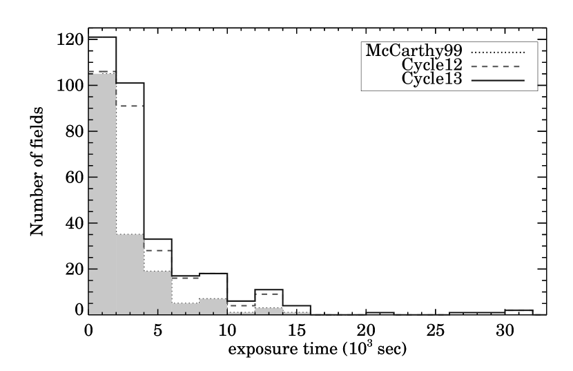
Figure 1: (Top): The distribution of exposure times of the observed fields in Cycles 7, 12, and 13. The shaded histogram with dotted lines is the data presented in McCarthy et al. (1999). The open histogram with dashed/solid line is the accumulated distribution when Cycles 12/13 data are added to the existing data. That is, the blue dashed line indicates the sum of Cycle 7 and Cycle 12 data, while the red solid line indicates the sum of Cycle 7, Cycle 12, and Cycle 13 data. (Bottom) : The histogram of $5\sigma$ line flux limits, within a 4-pixel aperture of the NICMOS grism data. Each pointing covers 0.75 arcmin². The line flux limits are compared to those from McCarthy et al. (1999), which is drawn with a dashed line.

We compare the exposure times of these 139 useable parallel fields taken during Cycles 12 and 13 with the earlier Cycle 7 survey in Figure 1a. Although the number of the deepest exposures is not significantly increased in Cycles 12 and 13, the number of total pointings is nearly double those from the Cycle 7 (Cycle 7 data comprises 85 pointings over $\sim 65$ arcmin²; McCarthy et al. 1999). In particular, the number of pointings with medium exposure times (2000–10000 seconds) have increased substantially.

We illustrate the distribution of $5\sigma$ line flux limits in Figure 1b. The rms noise in spectra-free regions is measured over a 4-pixel aperture for extracting one-dimensional spectrum. Thus, this “line flux limit” reflects the flux limit of a line added to the underlying continuum. As is expected from the exposure time comparison between Cycle 7 and Cycle 12/13 (Figure 1a), the line flux limits distribution of our data shows similar trend with that of Cycle 7. Though it is true that the fields with longer exposure time have fainter line flux limits, the depth of an image is not necessarily a simple function of the exposure time of an image. Instead, the flux limit is much more dependent on the flatness of the background, i.e., non-Poisson noise caused by imperfect background subtraction. Therefore, below $5\sigma$ flux limits, we don’t reliably identify emission lines because significant residuals remain from dark subtraction and other large data artifacts.

3 EMISSION-LINE GALAXIES

3.1 Identification

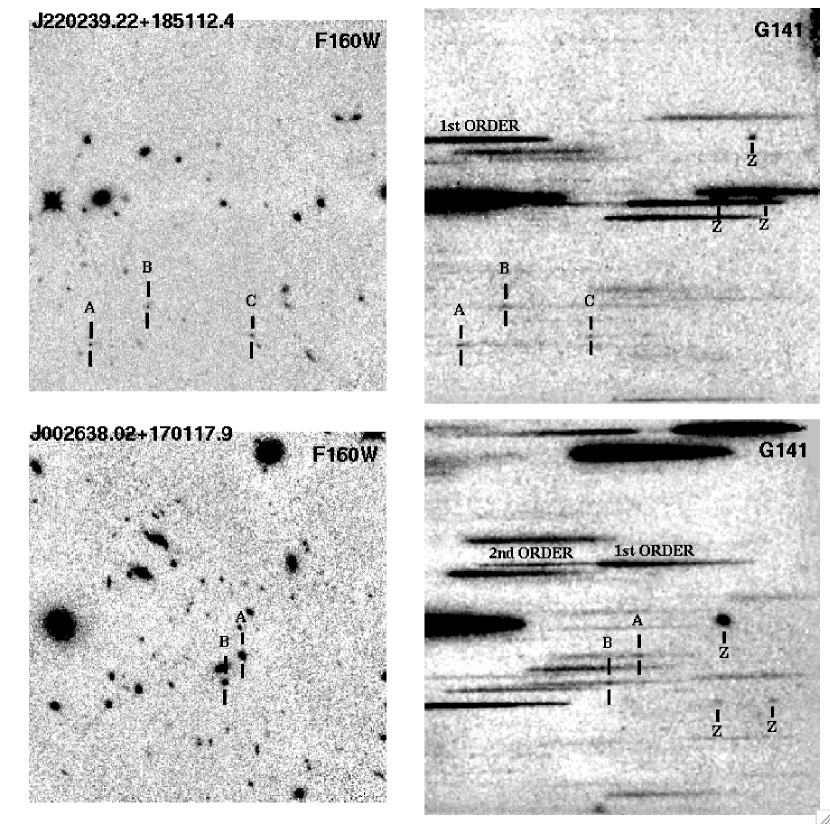
Figure 2: Typical pairs of direct (F160W) and grism (G141) images of our NICMOS parallel survey. Each field is $51.2\arcsec\times 51.2\arcsec$. In the grism two-dimensional image on the right, we mark the zero-order image (Z), the first and second order spectrum (1st order / 2nd order), and the emission lines. The objects producing the emission lines are also marked as A, B, or C in the direct image.

We identify the emission-line galaxy candidates on the two-dimensional spectra image through visual inspection, prior to the extraction of a one-dimensional spectrum using NICMOSlook (Section 2.2). We carefully compare the grism images and the direct images, identifying the galaxies in the direct images that are responsible for the emission-line in the spectra. We cross-check this method by identifying the same emission-line galaxies among multiple different authors. Some major obstacles in the identification of the emission-lines are the existence of zero-order images, the remaining background patterns, and the occasional image artifact. The zero-order image appears at a location $\sim 27\arcsec$ apart from the end of the first order spectrum, so it can be recognized in most cases through the inspection of the first-order spectrum or the inspection of direct images. However in the middle portion of the detector, it is difficult to tell whether the point-like feature is a zero-order image or a strong emission-line with faint continuum. Figure 2 shows two typical pairs of direct and grism images in our data and the identified emission-line galaxies. Zero-order images, the first and the second order spectrum, and the identified emission-line features are marked.

Over the $\sim 104$ arcmin² surveyed in Cycle 12 and Cycle 13, we identify 80 emission-line galaxies. As we mentioned in Section 2.3, we only classify an emission-line as real if the line is significant at $>5\sigma$ levels. Table 1 presents the coordinates, redshifts, line fluxes, observed equivalent widths, and available photometry of all 80 emission-line galaxies. The emission-line galaxies are distributed over 53 different fields, with 23 fields containing more than one emission-line galaxy.

The most likely candidates for the identified emission lines in our grism survey are hydrogen lines (H$\alpha$, H$\beta$) and oxygen lines ([OII] 3727Å, [OIII] 5007Å) redshifted to $z>0.7$. Because of the broad wavelength coverage of G141 (1.1–1.9$\mu$m), we would expect to see both [OIII] and H$\alpha$ in galaxies at $1.2<z<1.9$ and both [OII] and [OIII] in galaxies at $1.95<z<2.8$. Only a single line is predicted for H$\alpha$ at $z<1.2$ and [OII] at $z>2.8$. Except for ten possible cases discussed in Section 3.3, we do not convincingly detect more than one emission line in most of the galaxies. That is, the derivation of redshift depends on only a single strong emission line in most cases. We believe that most of these single lines are H$\alpha$ considering their large equivalent widths.

We can estimate the possibilities of the emission lines being emission lines other than H$\alpha$ using the expected equivalent widths of the lines, since our identification is limited to emission lines with EW (rest-frame) $>40$–50Å. First, the possibility of H$\beta$ line is removed since the average equivalent widths for H$\beta$ in star-forming galaxies are known to be relatively small (5–$10\mbox{\AA}$, Brinchmann et al. 2004). The next strongest line after H$\alpha$ in terms of equivalent width is [OII] 3727Å line. Identifying the emission line as [OII] 3727Å requires the redshift of the object to be $1.95<z<4$. Considering the typical magnitude of our emission-line galaxies, the $M_{V}$ should be $\sim-24$ mag if the galaxy is at $z\sim 3$. The estimated number of $z\sim 3$ galaxies with $M_{V}<-24$ over our survey volume is less than two according to the V-band luminosity function of $z\sim 3$ galaxies (Shapley et al. 2001), thus the possible contamination rate by [OII] lines at $z\sim 3$ is less than 3 percents (2/80). Furthermore, most [OII] contaminants will be in the $1.95<z<2.8$ range, where [OIII] 5007Å line should also appear in our spectra. We suggest this possibility for one object, J033310.66-275221.4a presented in Figure 4 in Section 3.3. This object is also included in Table 1 since the possibility of the line being [OII] instead of H$\alpha$ is still uncertain. Finally, the last possibility for contamination is the [OIII] 5007Å line. Yet as we mentioned in the previous paragraph, [OIII] 5007Å emission line is accompanied with either H$\alpha$ or [OII] 3727Å at $1.2<z<2.8$. Therefore the possibility of [OIII] being the single, strongest emission line of the galaxy is very low.

Besides these strong candidates, lines with longer wavelengths are also possible, including HeII $10830\mbox{\AA}$. However, these are not likely due to their weakness and the lack of accompanying nearby lines like [SIII] at $9069,9545\mbox{\AA}$. The follow-up optical spectroscopy targeting 14 emission-line galaxies presented in McCarthy et al.(1999) revealed that 9 of the emission-line galaxies are truly at $z=1$–2, supporting the identified emission lines through NICMOS grism spectroscopy are mostly redshifted H$\alpha$ (Hicks et al. 2002). The remaining 5 sources had no identifiable emission lines and were therefore unconfirmed, but not ruled out. In conclusion, we find that contamination from other emission lines is small ($\leq 5$%). Nonetheless, we include this source of uncertainty in the derivation of the H$\alpha$ luminosity function (Section 4).

In addition to mis-identification of emission lines, there is also a possibility of contamination by H$\alpha$ emission from AGN. We estimated the fraction of these contaminants using AGN luminosity function at similar redshifts and magnitudes. At $z\simeq 1$, the number density of Type-1 AGN with $\langle M_{B}\rangle\sim-23$ mag, corresponding to the median magnitude of our emission-line galaxies, is $\sim 10^{-5}$ Mpc^-3 (Bongiorno et al. 2007). Our effective survey volume is $\sim 3.14\times 10^{5}$ Mpc³ at this redshift range, which would indicate 3–4 AGNs in our survey. This is actually the lower limit on the AGN number density in our data, since for a given $H$-band continuum magnitudes, AGN candidates are likely to be brighter and thus easier to be included in the grism survey sample compared to normal star-forming galaxies, due to the larger intrinsic equivalent width of the H$\alpha$ line. Using the follow-up optical spectroscopy of the objects selected in the previous NICMOS grism survey, Hicks et al.(2002) suggested a new diagnostic for Seyfert 1 galaxies with L(H$\alpha$) and H$\alpha$ equivalent width. We have five objects within the conservative cut of log(L${}_{\mbox{H}\alpha}$)$>42.6$ erg s^-1 and EW(H$\alpha$)$>100\mbox{\AA}$, while we have five more objects with EW(H$\alpha$)$>100\mbox{\AA}$ and the luminosities of $42.5<$log(L${}_{\mbox{H}\alpha}$)$<42.6$ erg s^-1. We assume these numbers represent the possible uncertainties caused by AGN contamination.

To summarize, i) all the galaxies in the brightest bin (log(L${}_{\mbox{H}\alpha}$)$>42.8$ erg s^-1) can be considered AGNs according to the criteria of Hicks et al.(2002). ii) $\sim 40$% of the galaxies in the bin of $42.5<$log(L${}_{\mbox{H}\alpha}$)$<42.8$ erg s^-1 are possible AGNs with large equivalent widths. These uncertainties are included in Table 2, and in the derivation of the H$\alpha$ luminosity function.

3.2 H$\alpha$-Derived Star Formation Rates

Since H$\alpha$ and [NII] 6583Å, 6548Å are not deblended at the resolution of NICMOS grism, we correct the derived H$\alpha$ luminosity for [NII] contribution when we use H$\alpha$ luminosity as measures of star formation rate. The flux ratio used in correction is [NII] 6583/H$\alpha=0.3$ and [NII] 6583/[NII] 6548 $=3$ (Gallego et al. 1997). The H$\alpha$ luminosities used throughout this paper are derived from this corrected H$\alpha$ flux, derived using the following formula: $f_{c}(\mbox{H}\alpha)=0.71\times f(\mbox{H}\alpha+[\mbox{NII}])$. The star formation rates are derived from the corrected H$\alpha$ luminosity using the formula of Kennicutt (1998), which assume a Salpeter IMF between 0.1–100 M_⊙. Note that the star formation rate in Table 1 is not corrected for dust extinction.

In Figure 3, we show the distribution of H$\alpha$-derived star formation rates as a function of redshift and M_R. The H$\alpha$-inferred star formation rates of the identified emission-line galaxies are 2–200 $\mbox{M}_{\odot}\mbox{yr}^{-1}$, comparable to or larger than the UV-estimated star formation rates of typical $z\sim 3$ Lyman break galaxies with relatively little extinction (Shapley et al. 2001). We do not apply any dust extinction correction for the star formation rate of individual galaxies or our derivation of H$\alpha$ luminosity function, although $\langle A_{V}\rangle\sim 1$ mag is expected for H$\alpha$-selected star-forming galaxies (e.g., Kennicutt 1992). We only use this H$\alpha$ extinction correction for our estimates of star formation rate density evolution (see Section 5).

The redshifts of our sample galaxies span the range of $0.7<z<1.9$, with a steep decrease at the low-redshift ($z<0.9$) and high-redshift ends ($z>1.8$). This is expected from the sharp end of the G141 grism response curve. The median redshift is $\langle z\rangle=1.4$. The inhomogeneous redshift distribution is considered in the derivation of the luminosity function, but the effect is small.

Figure 3b illustrates the median absolute magnitude of $M_{R}\sim-22.5$ for our sample galaxies. The magnitude is comparable with $M_{B}^{*}=-22.8$ for galaxies at $z=1$–1.2 (Ryan et al. 2007). Therefore our galaxies have typical luminosities around $M^{*}$, across the entire redshift range. Despite considerable scatter, $M_{R}$ can be used as stellar mass indicator for a galaxy. Thus, the higher SFR for the brighter galaxies may indicate that between $1<z<2$, the star formation is higher in the more massive galaxies in our sample.

3.3 Spectra of Possible Double-Line Objects

We discussed in Section 3.1, the validity of identifying the single emission lines as H$\alpha$. If more than one emission line (i.e., two emission lines) exist, in nearly every case we identify them to be redshifted H$\alpha$ and [OIII] 5007Å based on the wavelength ratio between two emission lines. Using the known [OIII]/H$\alpha$ EW ratios of star-forming galaxies at $z\sim 0.7$, we predict the number of galaxies showing both H$\alpha$ and [OIII]. For a typical [OIII]/H$\alpha$ EW ratio of $\sim 0.4$ and our detection limit of EW(emission line)$>40$–50Å, the H$\alpha$ equivalent width required for [OIII] 5007Å line detection is $>120\mbox{\AA}$. Additionally, in order to show both [OIII]/H$\alpha$ lines in grism spectrum, the redshift of the object should be $1.2<z<1.9$ which corresponds to $\sim 60$% of the total survey volume. Thus, the expected number of galaxies with both H$\alpha$ and [OIII] 5007Å emission lines in this survey is $\sim 11$.

The actual number of galaxies in our sample with possible [OIII] and H$\alpha$ emission is eight or nine of the ten double-line objects. The line identification for one object is uncertain [J033310.66-275221.4a], and the other one [J121900.59+472830.9c] is likely a zero-order contaminant. The number is in good agreement with the expected $\sim 11$ H$\alpha$/[OIII] emitters. Figure 4 shows one-dimensional spectra of ten objects with plausible double-line features.

J014107.80-652849.1a – This object shows two emission lines at 1.73$\mu$m and 1.32$\mu$m although the line at 1.32$\mu$m is only marginally detected. These lines are likely redshifted H$\alpha$ and [OIII] at $z=1.63$. We could not derive a reliable flux for [OIII] line. According to the equivalent width and the luminosity of H$\alpha$ line, this object is not considered as a Seyfert 1 galaxy (see Section 3.1). The extended morphology (SExtractor CLASS_STAR $<0.8$) also disfavors the possibility of this object being an AGN.

J015240.44+005000.2a – This object shows two emission lines at 1.52$\mu$m and 1.16$\mu$m and both lines are significant. The lines are likely redshifted H$\alpha$ and [OIII] at $z=1.31$. The large H$\alpha$ luminosity and the equivalent width, as well as the point-like morphology suggest that this object may be an AGN. The broad and asymmetric shape of the line at 1.16$\mu$m could be a blend of [OIII] 5007Å and H$\beta$.

J033310.66-275221.4a – This object shows two emission lines at 1.32$\mu$m and 1.76$\mu$m, but the identification of these two lines is difficult because the wavelength ratio is uncertain. The measured flux ratio between the two lines $EW_{1.76\mu m}$/$EW_{1.32\mu m}$ is less than 1, so H$\alpha$ would be weaker than [OIII]. On the other hand, the two lines may be explained more easily by [OII] and [OIII] lines redshifted to $z=2.52$. The morphology of this object is clearly extended, and the relatively smaller object size (radius of $\sim 0.5\arcsec$) compared to other emission-line galaxies also suggests the possibility of this object at $z>2$. The optical photometry of this object is available in MUSYC data (Gawiser et al. 2006), although the quality of SED fitting is low and the derivation of photometric redshift is difficult for this object. In Table 1, we identify the line at 1.76$\mu$m as the H$\alpha$ redshifted to $z=1.68$. However, this object is an example of possible mis-identification in construction of emission-line galaxy sample, thus we include it in the uncertainties of the luminosity function in Section 4.

J033310.66-275221.4b – This object shows two emission lines at 1.83$\mu$m and 1.39$\mu$m although the line at 1.39$\mu$m is only marginally detected. The lines are likely redshifted H$\alpha$ and [OIII] at $z=1.788$. Judging from the clearly extended morphology and the combination of EW and luminosity of the H$\alpha$ line, we conclude that this object is a star-forming galaxy rather than AGN.

J121900.59+472830.9c – This object has a very bright broad line at 1.77$\mu$m, and a weak line at 1.31$\mu$m. These may be redshifted H$\alpha$ and H$\beta$ at $z=1.7$. However the line at 1.77$\mu$m is strong (corresponding to a luminosity of $L(\mbox{H}\alpha)=1.8\times 10^{43}\mbox{erg}\mbox{s}^{-1}$, roughly $\sim 5L^{*}$) and broad, so it might be from a zero-order image of an adjacent galaxy. The location of the potential counterpart for this possible zero-order image is out of the field of view of our direct image, so we cannot confirm clearly whether this is a zero-order image or a true emission line. On the other hand, if this line is indeed H$\alpha$, we measure a Balmer decrement of H$\alpha$/H$\beta$ = 9.1, implying $A_{V}=2.09$.

J122512.77+333425.1a – We see two lines at 1.57$\mu$m and 1.19$\mu$m, which we identify as redshifted H$\alpha$ and [OIII] at $z=1.39$. The measured flux ratio between the two lines is $f_{1.57\mu m}$/$f_{1.19\mu m}\sim 1.06$, which falls within the possible range of H$\alpha$/[OIII] values for star-forming galaxies. Moreover the equivalent width and the luminosity of H$\alpha$ line remove the possibility of this object being a Seyfert 1 galaxy. The object shows relatively symmetric but not compact morphology in the direct (F160W) image, thus providing support that this object is a star-forming galaxy rather than AGN.

J123356.44+091758.4a – This object shows two emission lines at 1.84$\mu$m and 1.38$\mu$m although the line at 1.38$\mu$m is very weakly detected. The lines are likely redshifted H$\alpha$ and [OIII] at $z=1.8$. The large size of this object, large H$\alpha$ EW and large H$\alpha$ luminosity suggest this object is a large galaxy being powered by AGN.

J125424.89+270147.2a – This object shows two emission lines at 1.88$\mu$m and 1.43$\mu$m. The lines are likely redshifted H$\alpha$ and [OIII] at $z=1.861$. Judging from the clearly extended morphology and the combination of EW and luminosity of H$\alpha$ lines, we conclude that this object is a star-forming galaxy rather than AGN.

J161349.94+655049.1a – In addition to the significant line at 1.9$\mu$m, the spectrum of this object shows a weak line at 1.43$\mu$m. These lines are likely redshifted H$\alpha$ and [OIII] at $z=1.9$, although the line at 1.43$\mu$m is only marginally detected. The line at 1.9$\mu$m has relatively large equivalent width (473Å). The spatial scale of the object is relatively large and shows a sign of substructure, so we classify it as a bright star-forming galaxy.

J213717.00+125218.5a – This object shows two lines at 1.68$\mu$m and 1.28$\mu$m, which are probably redshifted H$\alpha$ and [OIII] at $z=1.56$. The flux ratio between the two lines is $f_{1.68\mu m}$/$f_{1.28\mu m}\sim 1.55$, although the [OIII] line is weak. The morphology of this object in the F160W image is not classified as a point source (with CLASS_STAR less than 0.9 in SExtractor output), although it does not show any clear signs of interaction.

4 H$\alpha$ LUMINOSITY FUNCTION

We use the 1/$V_{\mbox{\tiny{max}}}$ method (Schmidt 1968) in order to construct the H$\alpha$ luminosity function. Although the redshift distribution of the galaxies is not homogeneous due to the sharp cutoff at low/high redshift end, we find the effect is negligible in the calculation of $V_{\mbox{\tiny{max}}}$. We begin by calculating the maximum comoving volume $V_{\mbox{\tiny{max}}}$ over which each galaxy could lie and be detected, including corrections for all of our sample selection biases: redshift, flux, and the location in the image. The equation used is as follows (see eqn [1] of Yan et al. 1999) :

$$V_{\mbox{max}}=\Omega(f_{\mbox{H}\alpha})\times\int_{z1}^{z2}C(f_{\mbox{H}\alpha},f_{\mbox{lim}})R(\lambda_{\mbox{H}\alpha})\frac{dV}{dz}dz$$ (1)

In the above equation, the differential comoving volume $dV/dz$ is integrated over the redshift range of [z1, z2]. The integration range is defined as $z1=\mbox{max}(z_{l},z_{\mbox{min}})$, $z2=\mbox{min}(z_{h},z_{\mbox{max}})$ while $z_{l}$ and $z_{h}$ indicate the lower/higher redshift ends limited by the spectral cutoff of the G141 response curve ($z_{l}=0.67$ and $z_{h}=1.9$). The quantities $z_{\mbox{min}}$ and $z_{\mbox{max}}$ are the minimum/maximum redshift the object can be detected. While max($z_{l},z_{\mbox{min}}$) is $z_{l}$ in general, the maximum redshift the object can be detected is determined by the measured object flux, according to the equation $D_{L}(z_{\mbox{max}})=D_{L}(z)[f_{\mbox{H}\alpha}/f_{\mbox{lim}}]^{1/2}$ where $D_{L}$ is the luminosity distance at redshift $z$, $f_{\mbox{H}\alpha}$ is the measured flux of the identified H$\alpha$ line, and $f_{\mbox{lim}}$ is the limiting line flux of the image (see Section 2.3.). The spectral cutoff $z_{l}$ and $z_{h}$ vary according to the location of the object in NICMOS grism field of view. Covering the whole wavelength range of 1.1–1.9$\mu$m is only possible when the object lies at central portion of the image. Therefore, we used different $z_{l}$ and $z_{h}$ according to the object location in the grism field of view.

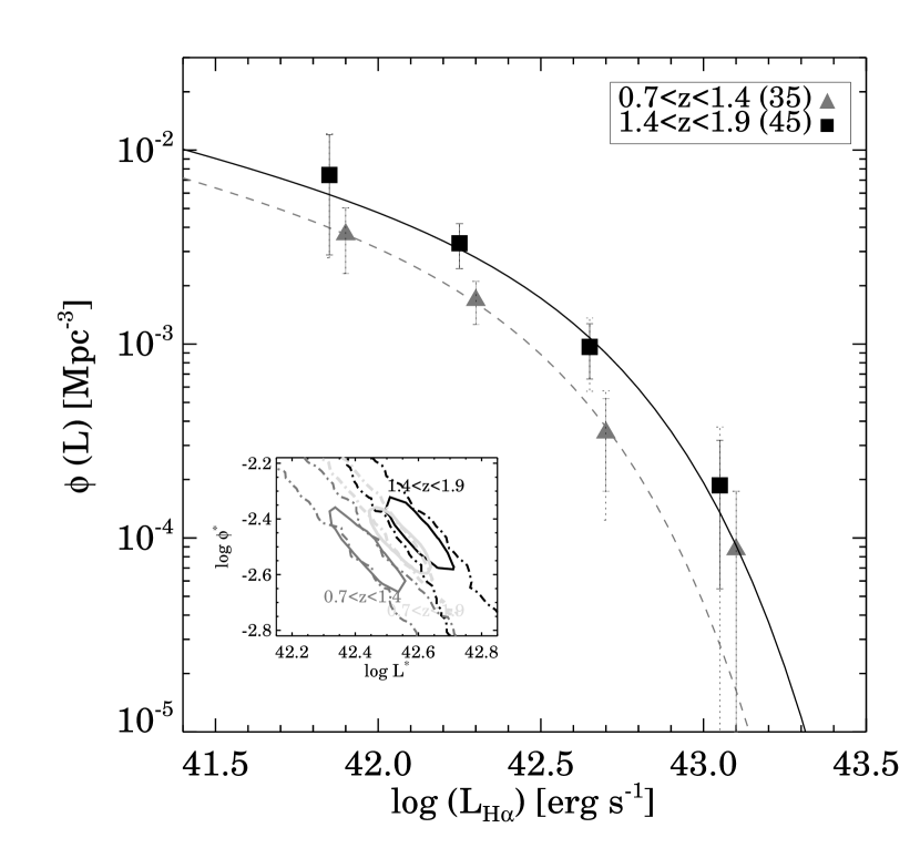
Figure 5: (Left): H$\alpha$ luminosity function over $0.7<z<1.9$ derived from our study of emission-line galaxies in NICMOS grism survey. The observed values are plotted as open circles, and the values after the incompleteness correction are plotted as filled circles. Error bars indicate Poisson (solid) and additional(dotted; uncertainties from line mis-identification, contamination) errors. Compared are Yan et al.(1999), Hopkins et al.(2000) points also from NICMOS grism studies (cross/triangle respectively). The solid line is the best-fit Schechter luminosity function to our derived luminosity function points, while the dotted line indicates the H$\alpha$ luminosity function of local galaxies (Gallego et al. 1995). (Right): H$\alpha$ luminosity function derived at two different redshift range ($0.7<z<1.4$, $1.4<z<1.9$). Overplotted solid and dashed lines are the best-fit Schechter luminosity function with the faint-end slope $\alpha$ fixed to $-1.39$. In the inset plot, the best-fit Schechter LF parameters for the two redshift-bin sub-samples are shown in addition to the Schechter parameters for $0.7<z<1.9$ samples. The solid contours indicate $1\sigma$ uncertainties in $L^{*}$ and $\phi^{*}$ when faint-end slope $\alpha$ is fixed, while dot-dashed contours indicate $1\sigma$ uncertainties when $\alpha$ is a free parameter.

The observed luminosity function needs to be corrected for sample selection biases, including redshift limits and the incompleteness. $R(\lambda)$ is the G141 inverse sensitivity curve, which corrects for the effect of the sharp spectral cutoff at the low- and high-redshift ends. Since we are using images with different depths, different incompleteness corrections must be applied for individual objects. $C(f_{\mbox{H}\alpha},f_{\mbox{lim}})$ is a factor for incompleteness correction assigned to each object, as a function of the observed H$\alpha$ line flux and the flux limit of the image. To estimate this correction factor, we first select several high S/N emission-line galaxies with different equivalent widths and wavelengths. After cutting out two-dimensional spectral templates of the selected emission-line galaxies, we dim the images by various factors to generate artificial emission-line galaxies with various line fluxes. The dimmed two-dimensional spectra are added to original NICMOS grism images at random locations, then we perform the one-dimensional spectral extraction, applying the same method that we described in Section 2.2. We repeat these steps for images with different $f_{\mbox{lim}}$ to measure $C(f_{\mbox{H}\alpha},f_{\mbox{lim}})$ as a function of galaxy location. We plot both uncorrected and corrected luminosity function in Figure 5a in order to show the significance of the incompleteness correction. Finally, $\Omega$ is the solid angle covered in this survey. $\Omega$ is also a function of $f_{\mbox{H}\alpha}$ since our objects are gathered from multiple images with widely differing line detection depths.

The source density in a specific luminosity bin of width $\Delta(\mbox{log}L)$ centered on the luminosity $\mbox{log}L_{i}$ is the sum of (1/$V_{\mbox{max}}$) of all sources within the luminosity bin (i.e., $\mbox{log}L_{i+1}-\mbox{log}L_{i}=2\times\Delta(\mbox{log}L)$). The variances are computed by summing the squares of the inverse volumes, thus the luminosity values and the error-bar in each bin is evaluated using the following equations.

$$\phi(\mbox{log}L_{i})=\frac{1}{\Delta(\mbox{log}L)}\sum_{|\mbox{log}L-\mbox{log}L_{i}|<\Delta(\mbox{log}L)}\frac{1}{V_{\mbox{max}}}$$ (2)

$$\sigma_{\phi}=\frac{1}{\Delta\mbox{log}L}\sqrt{\sum_{|\mbox{log}L-\mbox{log}L_{i}|<\Delta(\mbox{log}L)}\left(\frac{1}{V_{\mbox{max}}}\right)^{2}}$$ (3)

After calculating the size of the error-bars using the equation, we added additional uncertainties that might result from AGN contamination and line mis-identification (please refer to Section 3.1 for details). Note that the uncertainties in the luminosity function and the derived SFR density due to the large scale structure are less than $\sim 2$% (Trenti & Stiavelli 2008), given the large number of independent fields used in our survey. The derived luminosity functions from the whole sample ($0.7<z<1.9$) is presented in Figure 5a and Table 2, while the errors indicated already include additional uncertainties from AGN contamination and line mis-identification. The points from the previous NICMOS grism selected H$\alpha$ emitters (Yan et al. 1999; Hopkins et al. 2000) are overplotted for comparison, after accounting for the cosmology differences. Over the luminosity range of $41.6<\mbox{log}L(\mbox{H}\alpha)[\mbox{erg s}^{-1}]<43.5$, our LF is consistent with those of the previous studies. The solid line in Figure 5a is the best-fit Schechter LF to our data points, yet the line still fits points from other studies as well within the error bars. The plot shows a clear evolution of the H$\alpha$ LF from $z=1.4$ to the local H$\alpha$ LF (dotted line), a result already well-known from the luminosity evolution in other wavelengths like the UV (e.g., Arnouts et al. 2005).

The H$\alpha$ luminosity function we have derived is for galaxies with EW (rest-frame) $>40\mbox{\AA}$, as our survey is unable to confidently detect lines with lower equivalent widths. However, we note that our observed range of EWs is comparable to that of $z\sim 2$ star-forming galaxies observed in Erb et al.(2006). This suggests that there may be substantial overlap between our sample and the one reported by Erb et al.(2006), although our sample likely contains some dust obscured galaxies that would be missed by the UV selection of Erb et al.(2006).

The best-fit Schechter function parameters (Table 3) are derived using the MPFIT package, which provides a robust non-linear least square curve fitting (e.g., Ly et al. 2007). The errors in Table 3 correspond to $1\sigma$ uncertainty for each Schechter function parameter, and are derived using a Monte Carlo simulation. We generated a large number ($\sim 10000$) of Monte Carlo realizations of our LF, with different [log$L$, log$\phi$] sets perturbed according to the uncertainties. Then we repeat the fit to find the best-fit parameters for each realization of the LF. We find the faint-end slope is largely unconstrained by our data: $\alpha=-1.39\pm 0.43$. This is consistent with both the local H$\alpha$ LF ($\alpha=-1.35$; Gallego et al. 1995), and the deep NICMOS grism H$\alpha$ survey ($\alpha=-1.86\pm 0.14$; Hopkins et al. 2000). In addition to the Schechter function fitting with varying $\alpha$, we derived $L^{*}$ and $\phi^{*}$ with $\alpha$ being fixed to $-1.39,-1.0$ and $-1.8$ (Table 3) to cover all the possible range of $\alpha$, and to investigate the effect of varying $\alpha$ on the total SFR density derived.

Since the number of our sample galaxies (80) is more than twice of that from the previous studies, we can also test the evolution of H$\alpha$ LF as a function of redshift between 0.7 and 1.9. We divided the sample galaxies into two redshift bins ($0.7<z<1.4$, $1.4<z<1.9$), and derived the LFs separately. The LFs for two sub-samples at different redshift bin are shown in Figure 5b. The luminosity function in the lower-redshift bin ($0.7<z<1.4$; $\langle z\rangle=1.1$) is plotted as triangles, while the luminosity function for the higher-redshift bin ($1.4<z<1.9$; $\langle z\rangle=1.6$) is plotted as squares. We see that there are more H$\alpha$-luminous galaxies in the higher-redshift bin than in the lower-redshift bin, which implies that $L^{*}$, $\phi^{*}$, or both are larger at higher redshift.

The LF values and the best-fit Schechter parameters for these two redshift bins are also listed in Table 2 and 3. We also show the derivation of the Schechter parameters for the faint-end slope fixed at $\alpha=-1.39,-1.0,{\rm and}-1.8$ as this quantity is more difficult to constrain for these smaller sub-samples. The errors in $\phi^{*}$ and $L^{*}$ are derived by the same Monte Carlo method described above. For the cases where $\alpha$ is fixed, the uncertainties are artificially decreased, so we adopt the larger uncertainties derived when $\alpha$ is free. In the inset plot of Figure 5b, we illustrated how $\phi^{*}$ and $L^{*}$ evolve from $1.4<z<1.9$ to $0.7<z<1.4$. The contours represent the $1\sigma$ uncertainty range for the parameters (for $\alpha$ free and fixed, dot-dashed/solid line). The contours for parameters at $0.7<z<1.9$ is also illustrated.

5 EVOLUTION OF SFR DENSITY at $1<z<2$

From the derived LF parameters, we evaluate the H$\alpha$-inferred star formation rate density at $0.7<z<1.4$ (lower-redshift bin), and $1.4<z<1.9$ (higher-redshift bin). The SFR densities are also listed in Table 3. The total integrated H$\alpha$ luminosity density is calculated as $L_{\mbox{\tiny{tot}}}=\phi^{*}L^{*}\Gamma(\alpha+2)$, then converted to SFR density using the relation of Kennicutt (1998) : $SFR(H\alpha)[\mbox{M}_{\odot}\mbox{yr}^{-1}]=7.9\times 10^{-42}L(H\alpha)[\mbox{erg}\mbox{s}^{-1}]$. The relation assumes a Salpeter IMF between 0.1–100 M_⊙. The uncertainties in Table 3 are also derived through Monte Carlo method, by making a large realization of [$\phi^{*}$, $L^{*}$, $\alpha$] sets, calculating $L_{\mbox{\tiny{tot}}}$, and estimating $1\sigma$ uncertainty from the distribution of $L_{\mbox{\tiny{tot}}}$. As mentioned in previous section, the uncertainties on $L^{*}$ are underestimated for the cases where $\alpha$ is fixed.

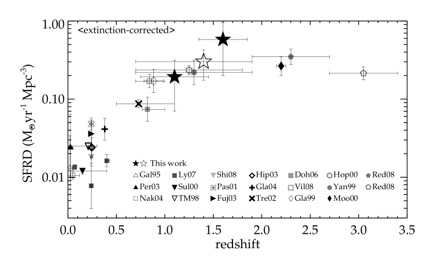
Figure 6: The evolution of SFR density as a function of redshift. Our points are plotted as two filled stars at $z=1.1$ and 1.6, produced from the integrated luminosity functions of the two sub-samples covering these redshift ranges. Also, the SFR density evaluated from the luminosity function over the entire range of $0.7<z<1.9$ is plotted at $z=1.4$ (open star). All other plotted points are based on the H$\alpha$-derived SFR density from spectroscopy or narrow-band imaging, (e.g., Gallego et al. 1995; Yan et al. 1999; Hopkins et al. 2000; Moorwood et al. 2000; Perez-Gonzalez et al. 2003; Sullivan et al. 2000; Tresse & Maddox 1998; Tresse et al. 2002; Pascual et al. 2001; Fujita et al. 2003; Nakamura et al. 2004; Hippelein et al. 2003; Glazebrook et al. 1999, 2004; Doherty et al. 2006; Ly et al. 2007; Shioya et al. 2008; Villar et al. 2008) except for points at $z=2.3$ and 3.05 (Reddy et al. 2008) who used H$\alpha$ luminosity function converted from UV luminosity function using a UV-H$\alpha$ relation.

We compare our SFR density estimates with the results of other studies in Figure 6. The SFR points are drawn from individual references (Gallego et al. 1995; Yan et al. 1999; Hopkins et al. 2000; Moorwood et al. 2000; Perez-Gonzalez et al. 2003; Sullivan et al. 2000; Tresse & Maddox 1998; Tresse et al. 2002; Pascual et al. 2001; Fujita et al. 2003; Nakamura et al. 2004; Hippelein et al. 2003; Glazebrook et al. 1999, 2004; Doherty et al. 2006; Ly et al. 2007; Shioya et al. 2008; Villar et al. 2008; Reddy et al. 2008; see compilation of Hopkins 2004), and were corrected to fit different cosmology. For extinction, we used the values given by the authors. The amount of the applied extinction correction is different for different studies, from $A(H\alpha)\sim 0.3$ mag to $A(H\alpha)\sim 1.2$ mag. This difference up to 1 magnitude produce the uncertainty in the SFR density points of a factor of $\sim 2$. If the authors do not provide information about the extinction, we apply the average extinction of $\langle A_{V}\rangle=1$ mag, i.e., $\langle A(H\alpha)\rangle\sim 0.85$ mag (e.g., Kennicutt 1992), the factor widely adopted in previous studies (e.g., Hopkins 2004; Doherty et al. 2006). The extinction correction applied to our SFR density points (stars in Figure 6) is also $\langle A(H\alpha)\rangle\sim 0.85$ mag.

Our estimate of the volume-averaged SFR density at $0.7<z<1.9$ is consistent with that of previous NICMOS grism studies over the same redshift range (points at $z=1.3$ from Yan et al. 1999; $z=1.25$ from Hopkins et al. 2000). Note that the integration ranges for H$\alpha$ luminosity density are different from study to study – our study accepts $L$ in the range $[0,\infty]$ while Hopkins et al.(2000) have integrated the LF over the range of $10^{37}<L[\mbox{erg}]<10^{47}$. Since the derived faint-end slope in our study is relatively flat ($1.39\pm 0.43$), this difference of integration range makes little difference in the final SFR density value. If we restrict the integration range to $10^{37}<L[\mbox{erg}]<10^{47}$ as in Hopkins et al.(2000), our result is decreased by only $\sim 0.1$%.

Our points clearly place the peak epoch of the relatively “unobscured” star formation at $z=1$–2. Moreover, by examining the two points at $z=1.1$ and $z=1.6$, we can conclude that the peak of star formation must have occurred at redshifts higher than $z=1.5$. This result is fairly robust, as it uses two sets of galaxies all identified with the same selection method.

6 SUMMARY

We have designed and executed a NICMOS grism survey, exploring the rest-frame optical universe at $0.7<z<1.9$. Through this program, we have identified a unique sample of emission-line galaxies over a significant cosmic volume, which enable us to study the relatively bright part of the H$\alpha$ luminosity function at $0.7<z<1.9$.

Using Cycle 12 and Cycle 13 data, we probe $\sim 104$ arcmin² area, at 139 different locations throughout the sky. This corresponds to an effective comoving volume of $\sim 3.14\times 10^{5}\mbox{Mpc}^{3}$, almost two times larger than that of our previous observations (McCarthy et al. 1999). We identified 80 probable emission-line galaxies, down to $L(\mbox{H}\alpha)\sim 4.4\times 10^{41}\mbox{erg}\mbox{s}^{-1}$. Most of the emission lines are thought to be redshifted H$\alpha$, and their $H$-band magnitude distribution suggests that the identified emission-line galaxies are relatively bright ($M\sim M^{*}$) star-forming galaxies at $0.7<z<1.9$.

We construct the H$\alpha$ luminosity function from the line fluxes and the redshifts of these galaxies. From the integration of the luminosity function, the luminosity density and the star formation rate density are derived. We divide our sample into two redshift bins, one at $0.7<z<1.4$ and the other at $1.4<z<1.9$. The volume-averaged star formation rate densities at these two different redshift range are evaluated to be $0.088\pm 0.056\mbox{M}_{\odot}\mbox{yr}^{-1}\mbox{Mpc}^{-3}$ and $0.265\pm 0.174\mbox{M}_{\odot}\mbox{yr}^{-1}\mbox{Mpc}^{-3}$ respectively. The results are consistent with other H$\alpha$-derived SFR densities at similar redshifts. Using our unique sample, all selected by the same method, we find that the cosmic star formation history probed by these H$\alpha$ measurements places the peak of star formation at $z>1.5$, with a decrease in global SFR density from $z=1.6$ to $z=1.1$. Although there remain uncertainties in the relative extinction, our study places firm constraints on the cosmic star formation history.

Table 1: Emission-line objects from the NICMOS grism survey

Field	Object	$\alpha$ (J2000)	$\delta$ (J2000)	redshiftHα	FluxHα	$W_{obs}$	F110W	F160W	logL${}_{\mbox{H}\alpha}$	SFR
					($10^{-16}$ erg s-1 cm-2)	(Å)	(mag)	(mag)	(erg s-1)	($\mbox{M}_{\odot}\mbox{yr}^{-1}$ )
J002638.02+170117.9	a	00:26:38.32	+17:01:20.7	1.206	2.653	320	23.13	22.52	42.24	13.8
$\cdots$	b	00:26:38.35	+17:01:24.8	1.300	1.299	230	23.48	22.61	41.97	7.4
J013433.61+311818.2	a	01:34:34.38	+31:18:05.3	1.283	3.372	283	22.20	22.20	42.38	19.0
$\cdots$	b	01:34:34.85	+31:17:56.0	1.657	5.546	281	24.47	23.26	42.73	42.8
J013510.41+313024.1	a	01:35:10.50	+31:29:31.3	1.441	1.545	350	–	23.42	42.10	10.0
J013655.80+153720.4	a	01:36:54.82	+15:37:27.8	1.083	2.827	139	22.72	22.21	42.21	12.9
$\cdots$	b	01:36:55.37	+15:37:51.5	0.773	3.645	334	21.93	21.57	42.14	11.0
J013916.84-002913.1	a	01:39:14.18	-00:28:38.9	0.888	2.870	185	–	22.29	42.11	10.2
$\cdots$	b	01:39:15.21	-00:28:23.6	1.407	4.291	322	–	21.24	42.53	27.1
$\cdots$	c	01:39:16.38	-00:28:33.6	1.651	2.453	244	–	21.68	42.38	18.8
J014107.80-652849.1	a	01:41:06.40	-65:28:25.6	1.641	5.248	249	–	22.59	42.70	40.0
$\cdots$	b	01:41:08.33	-65:28:26.1	1.047	6.941	172	–	23.80	42.58	30.4
J015108.44-832207.1	a	01:51:20.24	-83:22:00.7	1.593	2.706	254	22.67	23.39	42.40	19.9
J015240.44+005000.2	a	01:52:38.65	+00:50:45.0	1.314	4.811	271	–	21.59	42.55	27.9
J021011.32-043808.9	a	02:10:09.66	-04:38:14.3	1.128	2.386	148	–	22.88	42.16	11.4
J021017.37-043616.3	a	02:10:17.23	-04:36:12.4	1.564	4.152	467	23.57	22.90	42.58	29.8
$\cdots$	b	02:10:17.68	-04:36:36.5	1.043	0.947	122	24.43	23.59	41.72	4.1
J031951.03-191624.3	a	03:19:50.77	-19:16:46.2	0.974	4.848	217	21.87	21.36	42.38	19.4
J033309.36-275242.1	a	03:33:06.60	-27:52:05.4	1.370	0.897	287	–	24.59	41.84	5.5
$\cdots$	b	03:33:07.59	-27:52:40.9	1.590	1.779	285	–	23.12	42.22	13.0
J033310.66-275221.4	a	03:33:07.68	-27:51:47.1	1.681	0.881	135	–	24.63	41.94	6.9
$\cdots$	b	03:33:08.27	-27:51:47.8	1.788	1.482	334	–	24.02	42.20	12.6
J034932.44-533706.8	a	03:49:34.40	-53:37:23.1	1.465	4.250	325	22.48	21.45	42.55	28.2
J051917.75-454124.2	a	05:19:17.28	-45:41:30.9	1.648	0.462	136	23.20	21.96	41.65	3.5
$\cdots$	b	05:19:18.36	-45:40:59.7	1.169	2.792	248	22.40	21.83	42.25	14.0
J054709.71-505535.4	a	05:47:09.51	-50:55:56.9	1.110	1.410	228	–	–	41.92	6.6
J081955.60+421755.4	a	08:19:55.53	+42:17:50.5	1.122	0.958	156	23.61	22.56	41.76	4.6
J084830.53+444456.9	a	08:48:33.21	+44:45:27.4	1.445	2.663	284	–	22.56	42.34	17.4
$\cdots$	b	08:48:33.66	+44:45:33.4	1.073	2.936	208	–	22.49	42.22	13.2
J084846.69+444336.8	a	08:48:47.04	+44:43:37.1	0.986	1.591	222	22.36	21.97	41.91	6.5
J085828.67-161442.3	a	08:58:27.27	-16:14:30.2	1.158	1.252	180	23.46	22.45	41.90	6.2
$\cdots$	b	08:58:28.93	-16:14:46.6	1.206	7.510	315	22.08	21.42	42.69	39.1
J091100.06+173832.2	a	09:11:00.87	+17:38:56.5	1.333	2.795	184	22.72	21.91	42.32	16.5
J094841.23+673041.9	a	09:48:36.87	+67:30:46.7	1.435	2.310	331	–	22.11	42.28	14.9
$\cdots$	b	09:48:43.91	+67:30:59.2	1.180	1.401	256	–	24.74	41.95	7.1
J100603.06+350241.2	a	10:06:01.50	+35:02:42.9	1.620	0.914	430	–	24.27	41.94	6.9
$\cdots$	b	10:06:04.91	+35:02:45.1	1.081	4.423	109	–	22.84	42.41	20.1
J103316.56+231102.6	a	10:33:17.25	+23:11:54.5	1.519	0.956	126	–	23.03	41.92	6.6
$\cdots$	b	10:33:19.19	+23:11:40.0	1.372	12.496	298	–	22.84	42.99	76.4
J104703.10+122919.7	a	10:47:01.41	+12:30:06.1	0.811	4.687	265	–	20.82	42.28	15.0
$\cdots$	b	10:47:02.36	+12:29:35.6	1.482	3.175	542	–	21.79	42.43	21.3
J104849.15+462852.5	a	10:48:48.37	+46:28:57.0	1.632	3.292	445	–	23.49	42.50	24.9
J111942.69+513839.1	a	11:19:40.61	+51:38:55.8	1.733	1.689	219	23.09	22.00	42.24	13.8
J112413.26-170215.6	a	11:24:13.50	-17:02:14.1	1.744	0.719	185	23.94	23.47	41.87	5.9
$\cdots$	b	11:24:13.70	-17:02:33.2	1.349	2.517	443	23.53	22.34	42.28	15.1
J112414.50-170137.3	a	11:24:15.58	-17:01:45.9	1.667	1.041	185	23.79	23.02	42.01	8.1
J112846.94+641459.7	a	11:28:44.19	+64:15:06.3	1.005	1.467	137	23.62	23.75	41.89	6.1
$\cdots$	b	11:28:48.60	+64:15:00.5	1.559	2.655	177	22.58	23.33	42.38	19.0
J120513.71-073124.0	a	12:05:13.33	-07:30:54.9	1.550	0.722	190	–	25.18	41.81	5.1
J121900.59+472830.9	a	12:18:58.73	+47:28:16.6	1.679	1.751	236	–	–	42.24	13.7
$\cdots$	b	12:18:59.24	+47:28:10.9	1.462	4.513	115	22.92	22.16	42.58	29.8
$\cdots$	c	12:18:59.48	+47:28:10.8	0.996	3.779	200	21.63	21.06	42.29	15.5
J121936.36+471950.6	a	12:19:35.78	+47:19:35.8	1.186	1.391	220	–	24.56	41.95	7.1
J122226.64+042914.2	a	12:22:25.25	+04:28:35.9	1.601	0.556	106	–	22.88	41.72	4.1
J122246.79+155704.0	a	12:22:47.16	+15:56:45.2	1.697	0.853	126	22.94	22.09	41.93	6.8
J122512.77+333425.1	a	12:25:11.12	+33:34:31.7	1.392	1.950	148	22.68	21.72	42.19	12.1
$\cdots$	b	12:25:13.26	+33:34:14.3	1.479	1.402	209	23.89	22.55	42.08	9.4
J122908.41+015420.1	a	12:29:08.56	+01:54:08.5	1.752	1.868	171	–	20.96	42.29	15.4
J123041.86+121509.1	a	12:30:42.28	+12:15:26.9	1.475	2.437	188	–	22.40	42.31	16.3
J123356.44+091758.4	a	12:33:56.24	+09:17:54.0	1.800	14.161	371	–	20.75	43.18	120.9
J124339.45-341843.1	a	12:43:40.88	-34:18:20.6	1.050	3.115	146	22.58	21.87	42.24	13.7
J125424.89+270147.2	a	12:54:24.63	+27:02:05.2	1.861	2.837	211	–	22.51	42.50	25.2
J132745.26-311537.8	a	13:27:44.50	-31:16:07.5	1.240	2.566	251	23.56	23.13	42.24	13.8
J132820.08-313744.8	a	13:28:19.70	-31:37:42.2	1.280	1.474	274	22.68	21.84	42.02	8.3
J135835.94+623046.5	a	13:58:38.24	+62:30:55.8	1.476	0.638	203	23.44	22.88	41.73	4.3
J140214.22-113634.5	a	14:02:13.67	-11:36:53.1	1.514	0.711	215	23.09	22.85	41.79	4.9
J141833.44+250745.0	a	14:18:33.84	+25:07:45.1	1.419	1.629	215	24.48	24.39	42.12	10.4
J161349.94+655049.1	a	16:13:52.19	+65:50:51.4	1.904	6.688	473	–	23.66	42.89	61.2
$\cdots$	b	16:13:47.61	+65:50:35.0	1.748	0.692	195	–	–	41.86	5.7
J175907.13+664454.3	a	17:59:03.06	+66:45:13.0	1.331	1.620	178	24.56	24.72	42.08	9.5
$\cdots$	b	17:59:09.47	+66:44:48.9	1.614	1.618	190	25.12	24.13	42.18	12.1
$\cdots$	c	17:59:11.37	+66:44:41.9	1.446	0.640	131	24.11	23.67	41.72	4.2
J213717.00+125218.5	a	21:37:18.38	+12:51:34.8	1.561	6.620	226	–	20.85	42.78	47.4
J220239.22+185112.4	a	22:02:38.87	+18:51:37.9	1.406	2.759	312	–	23.40	42.34	17.4
$\cdots$	b	22:02:39.09	+18:51:29.3	1.505	4.187	484	23.72	23.13	42.56	28.7
$\cdots$	c	22:02:40.03	+18:51:24.5	1.663	1.678	242	24.62	23.60	42.22	13.0
J222640.90-722919.8	a	22:26:41.14	-72:29:14.3	1.692	1.477	191	–	20.95	42.17	11.7
J225916.39-345408.5	a	22:59:16.51	-34:54:11.5	1.507	2.931	254	–	22.39	42.41	20.1
J230342.56+085617.2	a	23:03:42.20	+08:56:42.9	1.355	5.527	156	22.46	21.59	42.62	33.3
$\cdots$	b	23:03:43.68	+08:56:07.4	1.164	0.799	581	23.33	23.00	41.70	4.0

Table 2: The derived H$\alpha$ luminosity function in grism survey

$z\sim$ 0.7–1.9				$z\sim$ 0.7–1.4				$z\sim$ 1.4–1.9
log$L$	$\phi$ (10${}^{-3}\mbox{Mpc}^{-3}$)	$N_{gal}$		log$L$	$\phi$ (10${}^{-3}\mbox{Mpc}^{-3}$)	$N_{gal}$		log$L$	$\phi$ (10${}^{-3}\mbox{Mpc}^{-3}$)	$N_{gal}$
41.8	$5.7115\pm 2.8134$	20		41.9	$3.6746\pm 1.3633$	13		41.85	$7.4484\pm 4.6620$	13
42.1	$3.2962\pm 0.7774$	26		42.3	$1.6812\pm 0.4203$	17		42.25	$3.3088\pm 0.8610$	20
42.4	$2.0319\pm 0.5149$	21		42.7	$0.3485\pm 0.2248$	4		42.65	$0.9663\pm 0.3960$	10
42.7	$0.6172\pm 0.2522$	10		43.1	$0.0871\pm 0.0871$	1		43.05	$0.1868\pm 0.1868$	2
43.0	$0.1202\pm 0.1202$	2
43.3	$0.0704\pm 0.0704$	1
		80				35				45

Note. — The uncertainties include Poisson errors, possible AGN contamination, and line mis-identification.

Table 3: H$\alpha$ luminosity function parameters for emission-line galaxies

$z$ range	$N_{gal}$	$\phi^{*}(10^{-3}\mbox{Mpc}^{-3})$	$\alpha$	$\mbox{log}L^{*}$	SFRD ($\mbox{M}_{\odot}\mbox{yr}^{-1}\mbox{Mpc}^{-3}$)
		$0.788\pm 0.881$	$-1.78\pm 0.46$	$42.72\pm 0.23$	$0.088\pm 0.056$
0.7–1.4	35	$2.704\pm 0.841$	$-1.39$ (fixed)	$42.48\pm 0.12$	$0.094\pm 0.023$
		$5.046\pm 1.125$	$-1.0$ (fixed)	$42.27\pm 0.09$	$0.074\pm 0.014$
		$0.848\pm 0.289$	$-1.8$ (fixed)	$42.79\pm 0.12$	$0.187\pm 0.033$
		$1.745\pm 1.578$	$-1.90\pm 0.39$	$42.72\pm 0.20$	$0.265\pm 0.174$
1.4–1.9	45	$4.096\pm 1.129$	$-1.39$ (fixed)	$42.54\pm 0.10$	$0.164\pm 0.034$
		$7.106\pm 1.851$	$-1.0$ (fixed)	$42.37\pm 0.09$	$0.129\pm 0.019$
		$1.491\pm 0.495$	$-1.8$ (fixed)	$42.80\pm 0.12$	$0.334\pm 0.063$
		$4.241\pm 3.553$	$-1.39\pm 0.43$	$42.46\pm 0.19$	$0.138\pm 0.058$
0.7–1.9	80	$3.303\pm 0.512$	$-1.39$ (fixed)	$42.54\pm 0.06$	$0.132\pm 0.012$
		$5.888\pm 0.514$	$-1.0$ (fixed)	$42.38\pm 0.03$	$0.112\pm 0.009$
		$1.122\pm 0.188$	$-1.8$ (fixed)	$42.82\pm 0.04$	$0.269\pm 0.021$

Note. — The values are calculated for $\Omega_{m}=0.3$, $\Omega_{\Lambda}=0.7$, and $h=71\mbox{km}\mbox{s}^{-1}\mbox{Mpc}^{-1}$. The adopted form of the luminosity function is $\phi(L)=\phi^{*}(L/L^{*})^{1+\alpha}\mbox{exp}(-L/L^{*})$. The SFR density column is inferred from the H$\alpha$ luminosity density, using $SFR(H\alpha)(\mbox{M}_{\odot}\mbox{yr}^{-1})=7.9\times 10^{-42}L(H\alpha)\mbox{erg}\mbox{s}^{-1}$ from Kennicutt (1998). Here, the total luminosity density is derived using the luminosity function parameters : $L_{\mbox{\tiny{tot}}}=\phi^{*}L^{*}\Gamma(\alpha+2)$.

Figure 3: (Left): Star formation rates of the emission-line galaxies as a function of redshift. The identified emission-line galaxies are distributed over $0.7<z<1.9$, with no significant redshift peak. (Right): Star formation rates of the emission-line galaxies as a function of absolute magnitudes $M_{R}$. $M_{R}$ magnitudes are derived from the observed $H$-band (F160W) magnitudes.

Figure 4: One-dimensional spectra of the galaxies which appear to have more than one emission line. In most cases, the emission lines are redshifted H$\alpha$ and [OIII] 5007Å (see Section 3.3 for details).

References

- (1) Arnouts, S. et al. 2005, ApJL, 619, 43
- (2) Bongiorno, A. et al. 2007, A&A, 472, 443
- (3) Bouwens, R. J., Illingworth, G. D., Blakeslee, J. P., & Franx, M. 2006, ApJ, 653, 53
- (4) Bouwens, R. J., Illingworth, G. D., Franx, M., & Ford, H. 2007, ApJ, 670, 928
- (5) Brinchmann, J., Charlot, S., White, S. D. M., Tremonti, C., Kauffmann, G., Heckman, T., & Brinkmann, J. 2004, MNRAS, 351, 1151
- (6) Dickinson, M., Papovich, C., Ferguson, H. C., & Budavaru, T. 2003, ApJ, 587, 25
- (7) Doherty, M., Bunker, A., Sharp, R., Dalton, G., Parry, I., & Lewis, I. 2006, MNRAS, 370, 331
- (8) Drozdovsky, I., Yan, L., Chen, H-W., Stern, D., Kennicutt, R., Spinrad, H., & Dawson, S. 2005, AJ, 130, 1324
- (9) Erb, D. K., Steidel, C. C., Shapley, A. E., Pettini, M., Reddy, N. A., & Adelberger, K. L. 2006, ApJ, 647, 128
- (10) Fontana, A. et al. 2004, A&A, 424, 23
- (11) Freudling, W. 1999, STECF, 26, 7
- (12) Freudling, W. et al. 2008, A&A, 490, 1165
- (13) Fujita, S. et al. 2003, ApJL, 586, 115
- (14) Gallego, J., Zamorano, J., Aragon-Salamanca, A., & Rego, M. 1995, ApJL, 455, 1
- (15) Gallego, J., Zamorano, J., Rego, M., & Vitores, A. G. 1997, ApJ, 475, 502
- (16) Gawiser, E. et al. 2006, ApJS, 162, 1
- (17) Glazebrook, K., Blake, C., Economou, F., Lilly, S., & Colless, M. 1999, MNRAS, 306, 843
- (18) Glazebrook, K., Tober, J., Thompson, S., Bland-Hawthorn, J., & Abraham, R. 2004, AJ, 128, 2652
- (19) Henry, A. L., Malkan, M. A., Colbert, J. W., Siana, B., Teplitz, H. I., McCarthy, P. J., & Yan, L. 2007, ApJL, 656, 1
- (20) Henry, A. L., Malkan, M. A., Colbert, J. W., Siana, B., Teplitz, H. I., & McCarthy, P. 2008, ApJL, 680, 97
- (21) Hicks, E. K. S., Malkan, M. A., Teplitz, H. I., McCarthy, P. J., & Yan, L. 2002, ApJ, 581, 205
- (22) Hippelein, H. et al. 2003, A&A, 402, 65
- (23) Hopkins, A. M., Connolly, A. J., & Szalay, A. S. 2000, AJ, 120, 2843
- (24) Hopkins, A. M. 2004, ApJ, 615, 209
- (25) Kennicutt, R. C. 1992, ApJS, 79, 255
- (26) Kennicutt, R. C. 1998, ARA&A, 36, 189
- (27) Ly, C. et al. 2007, ApJ, 657, 738
- (28) Madau, P., Pozzetti, L., & Dickinson, M. 1998, ApJ, 498, 106
- (29) McCarthy, P. et al. 1999, ApJ, 520, 438
- (30) Moorwood, A. F. M., van der Werf, P. P., Cuby, J. G., & Oliva, E. 2000, A&A, 362, 9
- (31) Nakamura, O., Fukugita, M., Brinkmann, J., & Schneider, D. P. 2004, AJ, 127, 2511
- (32) Noll, K, S. et al. 2004, proc.SPIE, 5487, 281
- (33) Pascual, S., Gallego, J., Aragon-Salamanca, A., & Zamorano, J. 2001, A&A, 379, 798
- (34) Perez-Gonzalez, P. G., Zamorano, J., Gallego, J., Aragon-Salamanca, A., & Gil de Paz, A. 2003, ApJ, 591, 827
- (35) Reddy, N. A., Steidel, C. C., Pettini, M., Adelberger, K. L., Shapley, A. E., Erb, D. K., & Dickinson, M. 2008, ApJS, 175, 48
- (36) Rudnick, G. et al. 2003, ApJ, 599, 847
- (37) Ryan, R. E. et al. 2007, ApJ, 668, 839
- (38) Shapley, A. E., Steidel, C. C., Adelberger, K. L., Dickinson, M., Giavalisco, M., & Pettini, M. 2001, ApJ, 562, 95
- (39) Shioya, Y. et al. 2008, ApJS, 175, 128
- (40) Schiminovich, D. et al. 2005, ApJL, 619, 47
- (41) Schmidt, M. 1968, ApJ, 151, 393
- (42) Steidel, C. C., Adelberger, K. L., Giavalisco, M., Dickinson, M., & Pettini, M. 1999, 519, 1
- (43) Sullivan, M., Treyer, M. A., Ellis, R. S., Bridges, T. J., Millard, B., & Donas, J. 2000, MNRAS, 312, 442
- (44) Trenti, M., & Stiavelli, M. 2008, ApJ, 676, 767
- (45) Tresse, L., & Maddox, S. J. 1998, ApJ, 495, 691
- (46) Tresse, L., Maddox, S. J., Le Fevre, O., & Cuby, J.-G. 2002, MNRAS, 337, 369
- (47) Villar, V., Gallego, J., Perez-Gonzalez, P. G., Pascual, S., Noeske, K., Koo, D. C., Barro, G., & Zamorano, J. 2008, ApJ, 677, 169
- (48) Yan, L., McCarthy, P., Freudling, W., Teplitz, H., Malumuth, E., Weymann, R., & Malkan, M. A. 1999, ApJL, 519, 47
- (49)