On the structure of correlations in the three dimensional spin glasses.

Abstract

We investigate the low temperature phase of three-dimensional Edwards-Anderson model with Bernoulli random couplings. We show that at a fixed value $Q$ of the overlap the model fulfills the clustering property: the connected correlation functions between two local overlaps decay as a power whose exponent is independent of $Q$ for all $0\leq|Q|<q_{EA}$. Our findings are in agreement with the RSB theory and show that the overlap is a good order parameter.

Spin glasses have unusual statistical properties. In mean field theory there are intensive quantities that fluctuate also in the thermodynamic limit. This is the effect of the coexistence of many equilibrium states. The correlations functions inside a given state should have a power law behavior: below the critical temperature spin glasses are always in a critical state (many glassy systems should share this behavior). These predictions of mean field theory have been never studied in details, apart from DGMMZ ; the aim of this paper is to address this point in a careful way.

In order to better characterize the behavior of spin glasses, it is convenient to consider two replicas, or clones, of the same system (let us call them $\sigma(i)$ and $\tau(i)$ where $i$ denotes the point of the lattice). The two clones share the same Hamiltonian $H_{J}$, the label $J$ indicates the set of random coupling constants.

Let us define the local overlap $q(i)\equiv\sigma(i)\tau(i)$ and the global overlap $q\equiv V^{-1}\sum_{i}q(i)$, $V$ being the total volume. For the three dimensional EA model EA at zero magnetic field (to be defined later) all simulations confirm that the probability distribution of $P_{J}(q)$ is non trivial in the thermodynamic limit, it changes from system to system and its average over the disorder, that we denote as $P(q)\equiv E[P_{J}(q)]$, is non trivial and it has a support in the region from $-q_{EA}$ to $q_{EA}$, $q_{EA}$ being the overlap of two generic configurations belonging to the same state. It is usually assumed that the function $P(q)$ has in the infinite volume limit a delta function singularity at $q=q_{EA}$, that appears as a peak in finite volume systems. In the presence of multiple states the most straightforward approach consists in identifying the clustering states (i.e. those where the connected correlation functions go to zero at large distance) and to introduce an order parameter that identifies the different states. This task is extremely difficult in a random system where the structure of the states depends on the instance of the system. However the replica theory is able to make predictions without finding out explicitly the set of states. At this end the introduction of the two clones plays a crucial role. Indeed if the global overlap $q$ has a preassigned value, the theory predicts that the correlations of local overlaps $q(i)$ go to zero at large distances. In other words $q$ is a good order parameter.

For each realization of the system we consider two clones. The observables are the local overlaps $q(i)$ and their correlations. We define $\langle O\rangle^{J}_{Q}$ the expectation value of the observable $O$ in the $J$-dependent Gibbs ensemble restricted to those configurations of the two clones that have global overlap $q=Q$. We define the average expectations values $\langle O\rangle_{Q}$ as weighted average over the systems of restricted expectation values :

$$\langle O\rangle_{Q}={E[P_{J}(Q)\langle O\rangle^{J}_{Q}]\over E[P_{J}(Q)]}\ .$$ (1)

The main statement of the RSB theory MPV (to which we bring evidence in this paper) is that the $Q$-dependent connected correlation functions go to zero when computed in the ensemble $\langle\cdot\rangle_{Q}$, i.e. the states $\langle\cdot\rangle_{Q}$ are clustering. The procedure is very similar to the one used in ferromagnetic models to construct clustering states (for example in the Ising case by considering averages with positive, or negative, total magnetization). The overlap constraint state is not clustering when the equilibrium state is locally unique (apart from a global change of signs) FH . Indeed this is the only known example of a system where the clustering states are labeled by a continuously changing order parameter in absence of a continuous symmetry, like rotations or translations.

This clustering property has far reaching consequences: for example the probability distribution $P(q)^{W}_{Q}$ of the window overlaps CINQUE , i.e. the average overlap over a region of size $W$, becomes a delta function in the infinite volume limit: $\lim_{W\to\infty}P(q)^{W}_{Q}=\delta(Q-q).$ Indeed when the region $W$ becomes large, the window overlaps are intensive quantities that do not fluctuate inside clustering states.

It is convenient to recall the known theoretical results for the connected correlation functions in the case of short range Ising spin glasses:

$$G(x|Q)=\langle q(x)q(0)\rangle_{Q},\ \ \ \ \ \ C(x|Q)=G(x|Q)-Q^{2}$$ (2)

and their Fourier transforms $\tilde{C}(k|Q)$.

Figure 1: The correlation function at distance 10 $G(10|Q)$ averaged in 20 bins (round points) and in ten bins (crosses) of $Q^{2}$, versus the average of $Q^{2}$ inside the bin. The data are for a system of size 20 and the straight is the best fit to the data.

The simplest predictions are obtained starting from mean field theory and computing the first non trivial term DKT Neglecting logarithms we have in the small $k$ region

$$\tilde{C}(k|Q)\propto k^{-4}\ \ \ \ \ \ \ Q=0\ ,$$ for

$$\tilde{C}(k|Q)\propto k^{-3}\ \ \ \ \ \ \ 0<Q<q_{EA}\ ,$$ for

$$\tilde{C}(k|Q)\propto k^{-2}\ \ \ \ \ \ \ Q=q_{EA}\ ,$$ for

$$\tilde{C}(k|Q)\propto(k^{2}+\xi(Q)^{-2})^{-1}\ \ \ \ \ \ \ Q>q_{EA}\ .$$ for (3)

These results are supposed to be exact at large distances in sufficiently high dimensions, i.e. for $D>6$.

The reader may be surprised to find a result for $Q>q_{EA}$ because the function $P(q)$ is zero in this region in the infinite volume limit. However for finite systems $P(q)$ is different from zero for any $q$ albeit it is very small FPV ; BFM in the region $q>>q_{EA}$. For $Q>q_{EA}$ an analytic computation of the function $\tilde{C}(k|Q)$ has not yet been done, however it is reasonable that the leading singularity near to $k=0$ in the complex plane is a single pole, leading to an exponentially decaying correlation function .

When the dimensions become smaller than $6$ we can rely on the perturbative expansion in $\epsilon=6-D$, where only the first order is (partially) known TD . It seems that predictions at $Q=q_{EA}$ should not change and the form of the $k=0$ singularity at $Q=q_{EA}$ (i.e. when the two clones belong to the same state) remains $k^{-2}$ as for Goldstone Bosons. On the contrary the $k=0$ singularities at $Q<q_{EA}$ should change. We can expect that

$$\tilde{C}(k|Q)\propto k^{-\tilde{\alpha}(Q)}\ \ \ \mbox{for}\ \ \ \ 0\leq Q<q_{EA}\ .$$ (4)

These perturbative results are the only information we have on the form of $\tilde{\alpha}(Q)$. The simplest scenario would be that $\tilde{\alpha}(Q)$ is discontinuous at $Q=0$ and constant in the region $0<Q<q_{EA}$. It would be fair to say that there is no strong theoretical evidence for the constancy of $\tilde{\alpha}(Q)$ in the region $0<Q<q_{EA}$, apart from generic universality arguments. On the contrary the discontinuity at $Q=0$ could persist in dimensions not too smaller than 6, and disappear at lower dimensions, as supported by our data in $D=3$.

In three dimensional case in configuration space we should have:

$$C(x|Q)\propto x^{-\alpha(Q)}\ \ \ \mbox{for}\ \ \ \ 0\leq Q\leq q_{EA}\ .$$ (5)

with $\alpha(q_{EA})=1$ (indeed in general we have that $\alpha(Q)=D-\tilde{\alpha}(Q)$). For $Q>q_{EA}$ the correlation should go to zero faster than a power: we tentatively assume that

$$C(x|Q)\propto x^{-1}\exp(-x/\xi(Q))\ \ \ \mbox{for}\ \ \ \ q_{EA}<Q\ ,$$ (6)

(also other behaviours are possible).

In this paper we will numerically study the properties of the two overlaps connected correlations functions in the three dimensional EA model. The Hamiltonian of the EA model EA is given by $H_{\sigma}=-\sum_{|i-j|=1}J_{i,j}\sigma_{i}\sigma_{j}$with $J_{i,j}=\pm 1$ (symmetrically distributed) and Ising spins $\sigma_{i}=\pm 1$.

Figure 2: Circles are the value of the exponent $\alpha(Q)$ by fitting $\chi^{(s)}(Q)_{L}$ as a power of $L$: for each value of $Q^{2}$ we show two points corresponding to $s=1$ and to $s=2$. Squares represent the same quantity $\alpha(Q)$ as obtained through the scaling approach visible in fig. 3.

We have studied cubic lattice systems with periodic boundary conditions of side $L$ for $L=4,6,8,10,12,16,20$. The simulation parameters are the same used in reference CGGPV . We present the results only at temperature $T=0.7$, while the critical temperature is about $T=1.11$.

We have first classified the configurations created during the numerical simulations according to the value of the global overlap $q$. Since the properties of the configurations are invariant under the symmetry ($q\to-q$), we have classified the configurations into 20 equidistant bins in $q^{2}$: e.g. the first bin contains all the configurations where $0<q^{2}<1/20$. In this way we compute the correlations $C(x|Q)$. We have measured the correlations only along the axes of the lattice: $x$ is an integer restricted to the range $0,L/2$. As a control we have done the same operation with 10 bins obtaining similar results.

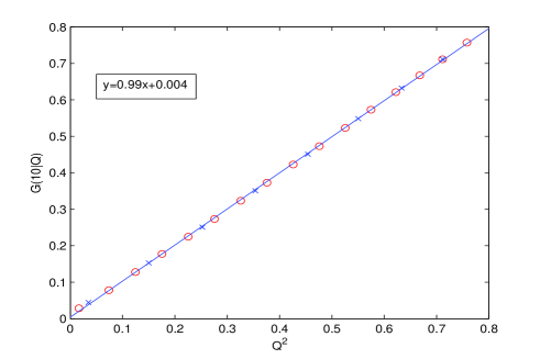
We have firstly verified that the connected correlations vanish for large systems. At this end in fig. (1) we have plotted for $L=20$ (our largest system) the correlation $G(10|Q)$ versus the average of $Q^{2}$ in the bin. We see that the two quantities coincide. The data show a strong evidence for the vanishing of the connected two point correlation function. The predictions of replica theory is $G(10|Q)=Q^{2}$, neglecting small corrections going to zero with the volume.

Further information can be extracted from the data. The analysis of the data should be done in a different way in the two regions $0\leq Q^{2}\leq q_{EA}^{2}$ and $q_{EA}^{2}<Q^{2}$ as far as two different behaviour are expected. In our case $q_{EA}^{2}$ can be estimated to be around $0.4$.

Figure 3: The quantity $L^{\alpha(Q)}C_{L}(x|Q)g(x/L)$ with $g(z)=(1/z+1/(1-z))^{-\alpha(Q)}$ versus $\sin(\pi x/L)$ for the set of data in the first bin $Q^{2}<0.5$, using the best value of $\alpha(Q)$. The left panel display the data for all the correlation at distances $x\geq 1$ (the corresponding value of $\alpha(Q)$ being 0.50); in the right panel we have only the data with $x\geq 2$ (the corresponding value of $\alpha(Q)$ being 0.54).

In the region $0\leq Q^{2}\leq q_{EA}^{2}$ the power law decrease (5) of the correlation is expected. To test this hypothesis JANUS we define for each $L$ the quantities $\chi^{(s)}_{L}(Q)$

$$\chi^{(s)}_{L}(Q)=\sum_{x=1}^{L/2}x^{s}C_{L}(x|Q).$$ (7)

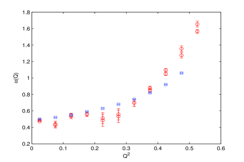
where $C_{L}(x|Q)$ is the connected correlation function in a system of size $L$, i.e. $G_{L}(x|Q)-Q^{2}$ . For large $L$ $\chi^{(s)}_{L}(Q)$ should behave as $L^{s+1-\alpha(Q)}$. We have evaluated the previous quantity for $s=1,2$. In the region $Q^{2}<0.4$ we have found that the ratio $\chi^{(2)}_{L}(Q)/\chi^{(1)}_{L}(Q)$ is well linear in $L$. Here the data for $\chi_{L}^{(s)}(Q)$ can be well fitted as a power of $L$ and the exponents $\alpha(Q)$ computed using $s=1$ and $s=2$ coincide within their errors. These results are no more true in the region $0.5<Q^{2}$ indicating that a power law decrease of the correlation is not valid there. The exponents we find with this method are shown in fig. (2).

In order to check these results for $\alpha(Q)$ we have used a different approach. In the large volume limit the correlation function should satisfy the scaling

$$L^{\alpha(Q)}C_{L}(x|Q)=f(x/L).$$ (8)

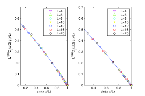
The value of $\alpha(Q)$ can be found by imposing this scaling. At this end for each value of $Q$ we have plotted $L^{\alpha(Q)}C_{L}(x|Q)$ and found the value of $\alpha(Q)$ for which we get the best collapse. The result of the collapse is shown in fig. (3) for $Q$ around zero, where for graphical purpose we have plotted $L^{\alpha(Q)}C_{L}(x|Q)g(x/L)$ versus $\sin(\pi x/L)$, where the function $g$ has been added to compress the vertical scale (we find convenient to use $g(z)=(1/z+1/(1-z))^{-\alpha(Q)}$, following MaPa ). In the left panel we show the collapse using all points with $x\geq 1$, in the right panel we exclude the correlations at distance $x=1$. The corresponding values of the exponent are shown in fig. (2) and they agree with the ones coming from the previous analysis in the region of $Q^{2}\leq 0.4$.

The exponent $\alpha(Q)$ is a smooth function of $Q^{2}$ which goes to 1 near $Q^{2}=0.4$ in very good agreement with the theoretical expectations. We do not see any sign of a discontinuity at $Q=0$, and this is confirmed by an analysis with an high number of bins (e.g. 100). However it is clear that for lattice of this size value we cannot expect to have a very high resolution on $Q$ and we should look to much larger lattices in order to see if there is a sign of a building up of a discontinuity and of a plateaux. The value of the exponent that we find at $Q=0$ is consistent with the value 0.4 found from the dynamics JANUS , and with the value 0.4 found with the analysis of the ground states with different boundary conditions MaPa .

Figure 4: The connected correlation $C_{L}(x|Q)$ as function of $Q^{2}$ for $x=6,7,8,9$ at $L=20$. The straight lines are linear fits.

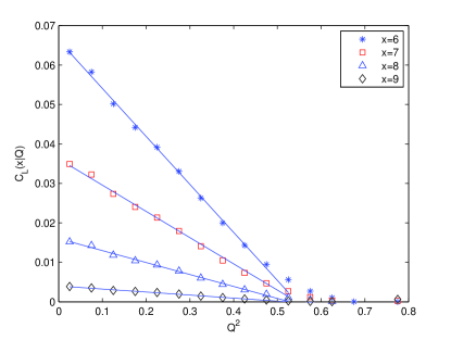
From the previous analysis it is not clear if the exponent $\alpha(Q)$ has a weak dependence on $Q$ or if the weak dependence on $Q$ is just a pre-asymptotic effect. In order to clarify the situation it is better to look to the connected correlations themselves. In fig. (4) we display the connected correlation $C_{L}(x|Q)$ as function of $Q^{2}$ for $x=6,7,8,9$ at $L=20$, our largest lattice (for the result at $x=1$ see CGGV ). We can fit the correlations at fixed $L$ (e.g. $L=20$) for large $x$ as:

$$C_{L}(x|Q)=A(x,L)(Q^{2}-B(x,L)^{2})\,,\ \ Q^{2}<B(x,L)^{2}$$ (9)

while $C_{L}(x|Q)$ is very near to zero for $Q^{2}>B(x,L)^{2}$. The goodness of these fits improves with the distance (similar results are valid at smaller $L$). The value of $B(x,L)^{2}$ is near to $q_{EA}^{2}$ and it is slightly decreasing with $L$. The validity of the fits (9) for large $L$ would imply that in the region $|q|<q_{EA}$ the large distance decrease of the correlation function should be of the form $A(Q^{2}-q_{EA}^{2})f(x)$ and therefore the exponent $\alpha(Q)$ should not depend on $Q$.

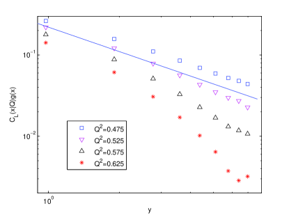
However near $q=q_{EA}$ we should have a real crossover region. In Fig. 5 we show $C_{L}(x|Q)g(x)$ at $L=20$ for $0.475\leq Q^{2}\leq 0.625$, versus $y\equiv(1/x+1/(2L-x))^{-1}$ (we use the variable $y=x(1-O(x/L))$ to take care of finite volume effects) with $g(x)=(1-2x/L)^{-2}$. It seems that the data at $Q^{2}>0.475$ decrease faster than a power at large distances and that the data at $Q^{2}=0.475$ are compatible with a power with exponent $-1$ It is difficult to extract precise quantitative conclusions, without a careful analysis of the $L$ dependence. We hope that this will be done when the data on the correlation functions on larger lattices will be available.

In the region $q_{EA}^{2}\leq Q^{2}$ our task is different: the correlations are short range and we would like to compute if possible the correlation length. At this end we have fitted the data as

$$C_{L}(x|Q)={a\over x+1}\exp(-x/\xi_{L}(Q))+(x\to L-x)+const$$ (10)

The choice of the fit is somewhat arbitrary, however we use it only to check that the correlation length diverges at $q_{EA}$ and that near $q_{EA}$ are well fitted by a $1/x$ power. The fits are good, but this may not imply the correctness of the functional form in eq. (10). We find that far from $Q=0.5$ the correlation length is independent of $L$, (it is quite small). We have tried to collapse the data for $L>8$ in the form

$$\xi_{L}(Q)=L\,f((Q^{2}-q_{EA}^{2})L^{1/\nu})\ .$$ (11)

A reasonable collapse has been obtained, however the $q_{EA}^{2}$ is quite small (i.e. 0.25): it is quite possible that there are finite volume effects and different ways to evaluate $q_{EA}$ give different results on a finite lattice and they would converge to the same value in the infinite volume limit.

Figure 5: Correlations functions at $L=20$ for $q^{2}$ = 0.475, 0.525, 0.575, 0.625, versus $y\equiv(1/x+1/(2L-x))^{-1}$. The straight line is proportional to $y^{-1}$.

In conclusion the global overlap for a two clone system is a well defined order parameter such that in the appropriate restricted ensemble the two points connected correlation function decays at large distance. The connected correlations decay as a power whose exponent seem to be independent from $Q$ for $0\leq|Q|<q_{EA}$: the value of the exponent is in agreement with the results obtained in different context at $Q=0$. Moreover the connected two points correlation functions at $Q=q_{EA}$ decays like $1/x$ in agreement with the detailed predictions coming from replica theory.

Acknowledgments. We thank E.Marinari. P. Contucci acknowledge STRATEGIC RESEARCH GRANT from University of Bologna. C. Giardinà and C. Vernia acknowledge GNFM-INdAM for partial financial support.

References

- (1) M. Mezard, G. Parisi, M.A. Virasoro, Spin Glass Theory and Beyond World Scientific, Singapore (1987).
- (2) D.S. Fisher and D.A. Huse, Phys. Rev. Lett. 56, 1601 (1986)
- (3) S.F. Edwards and P.W. Anderson, Jou. Phys. F., 5, 965, (1975).
- (4) E. Marinari, G. Parisi, F. Ricci-Tersenghi, J. Ruiz-Lorenzo and F. Zuliani, J.Stat. Phys. 98, 973 (2000).
- (5) P. Contucci, C. Giardinà, C. Giberti, C. Vernia Phys. Rev. Lett. 96, 217204 (2006)
- (6) E. Marinari, G. Parisi, Phys. Rev. B 62 (2000) 11677, Phys. Rev. Lett. 86 (2001) 3887.
- (7) C. De Dominicis, I. Giardina, E. Marinari, O. Martin and F. Zulliani. Phys. Rev. B 72 014443 (2005)
- (8) P. Contucci, C. Giardinà, C. Giberti, G. Parisi, C. Vernia Phys. Rev. Lett. 99, 057206 (2007)
- (9) C. De Dominicis, I. Kondor, and T. Temesvari, Beyond the Sherrington-Kirkpatrick Model (World Scientific, 1998), vol. 12 of Series on Directions in Condensed Matter Physics,p.119, cond-mat/9705215; Eur. Phys. J. B 11, 629 (1999).
- (10) S. Franz, G. Parisi and M. Virasoro, J. Phys. I (France) 2 (1992) 1869.
- (11) A. Billoire, S. Franz and E. Marinari J. Phys. A 36, 15-27 (2002)
- (12) T. Temesv ari and C. De Dominicis, Phys. Rev. Lett. 89, 097204 (2002); C. de Dominicis and I. Giardina Random Fields and Spin Glasses, Cambridge University Press 2006.
- (13) F. Belletti et al.,Phys. Rev. Lett. 101 (2008) 157201