Fluctuation and dissipation dynamics in fusion reactions
from stochastic mean-field approach

Abstract

By projecting the stochastic mean-field dynamics on a suitable collective path during the entrance channel of heavy-ion collisions, expressions for transport coefficients associated with relative distance are extracted. These transport coefficients, which have similar forms to those familiar from nucleon exchange model, are evaluated by carrying out TDHF simulations. The calculations provide an accurate description of the magnitude and form factor of transport coefficients associated with one-body dissipation and fluctuation mechanism.

I INTRODUCTION

The self-consistent mean-field theory, also known as time-dependent Hartree-Fock (TDHF), by employing Skyrme-type effective interactions, has been extensively applied to describe nuclear collision dynamics at low bombarding energies below 10 MeV per nucleon Ring ; Goeke ; Davis ; Sim08 . In the mean-field theory, short range two-body correlations are neglected and nucleons move in the self-consistent potential produced by all other nucleons. This is a good approximation at low energies since Pauli blocking is very effective for scattering into unoccupied states. Consequently, in the mean-field theory, collective energy is converted into intrinsic degrees of freedom via interaction of nucleons with the self-consistent mean-field, so-called one-body dissipation Koonin ; Negele . One-body dissipation mechanism plays dominant role in low energy nuclear dynamics including deep-inelastic heavy-ion collisions and heavy-ion fusion reactions. One important limitation of the mean-field theory is related with dynamical fluctuations of collective motion. In the mean-field description, while single-particle motion is treated in quantal framework, collective motion is treated almost in classical approximation. Therefore, TDHF provides a good description for average evolution, however it severely underestimates fluctuations of collective variables.

On the other hand, it is well known that no dissipation takes place without fluctuations Gardener ; Weiss . Much effort has been done to improve one-body transport description beyond the mean-field. Most of these transport descriptions take into account dissipation and fluctuation mechanisms due to two-body collisions, which play an important role in nuclear dynamics at intermediate energies Ayik1 ; Randrup1 ; Abe ; Lac04 . Here, we deal with nuclear dynamics at low energies at which one-body dissipation and associated mean-field fluctuations play a dominant role in dynamical evolution. One of the fundamental questions is how to improve the mean-field theory by incorporating one-body fluctuation mechanism at a microscopic level? In a recent work, based on an appealing idea of Dasso Dasso1 ; Dasso2 , this question has been addressed. A stochastic mean-field (SMF) approach has been proposed for describing fluctuation dynamics Ayik2 ; Ayik3 . For small amplitude fluctuations, this model gives a result for dispersion of a one-body observable that is identical to the result obtained through a variational approach Bal84 . It is also shown that, when the SMF is projected on a collective variable, it gives rise to a generalized Langevin equation Mori , which incorporates one-body dissipation and one-body fluctuation mechanisms in accordance with quantal dissipation-fluctuation relation. These illustrations give a strong support that the SMF approach provides a consistent microscopic description for dynamics of density fluctuations in low energy nuclear reactions. In this paper, we present another demonstration of the SMF approach.

In a recent work, by a suitable definition of collective variables of relative motion, the nucleus-nucleus potential energy and one-body friction coefficient as a function of relative distance have been extracted from simulations of microscopic TDHF Washiyama1 , see also Umar . Such a reduction is not constrained by adiabatic or diabatic approximation, therefore it should provide an accurate description of conservative nucleus-nucleus potential energy and the magnitude of the one-body dissipation mechanism Washiyama2 . It is of great interest to deduce magnitude of diffusion coefficients associated with collective variables. However, this information is not contained in the standard mean-field approximation. The SMF approach provides a proper framework for extracting dissipation and fluctuation properties of collective variables. In this work, we carry out a similar macroscopic reduction of the SMF approach on a collective path. In this manner, we deduce not only nucleus-nucleus potential and one-body friction coefficient, but also one-body diffusion coefficients associated with collective variables.

In Sec. II, we give a brief description of the SMF approach. In Sec. III, we present a suitable definition of collective variables in heavy-ion collisions, and the correlation function of Wigner distribution. In Sec. IV, we derive transport coefficients associated with relative motion from the SMF approach. In Sec. V, conclusions are given.

II STOCHASTIC MEAN-FIELD APPROACH

In the standard TDHF, temporal evolution of the system is described by a single Slater determinant constructed with time-dependent single-particle wave functions $\Phi_{j\sigma\tau}(\bm{r},t)$. Evolution of single-particle wave functions are determined by the TDHF equations with proper initial conditions,

$$i\hbar\frac{\partial}{\partial t}\Phi_{j\sigma\tau}(\bm{r},t)=h(\rho)\Phi_{j\sigma\tau}(\bm{r},t),$$ (1)

where $h(\rho)$ denotes the self-consistent mean-field Hamiltonian with the one-body density $\rho$. For clarity of notation spin-isospin quantum numbers $\tau=($proton, neutron$)$ and $\sigma=($spin-up, spin-down$)$ are explicitly indicated in these expressions. In many situations, it is more appropriate to express the mean-field approximation in terms of the single-particle density matrix,

$$\rho(\bm{r},\bm{r}^{\prime},t)=\sum\limits_{j\sigma\tau}\Phi_{i\sigma\tau}^{\ast}(\bm{r},t)n_{j}^{\sigma\tau}\Phi_{j\sigma\tau}(\bm{r}^{\prime},t),$$ (2)

where $n_{j}^{\sigma\tau}$ denotes occupation factors of single-particle states. In the standard TDHF, occupation factors are one and zero for the occupied and unoccupied states, respectively. If the initial state is at a finite temperature, the average occupation factors are determined by the Fermi-Dirac distribution.

TDHF provides a deterministic evolution of the single-particle density matrix, starting from a well-defined initial state and leading to a well-defined final state. In order to incorporate fluctuation mechanism into dynamics, we give up standard description in terms of a single Slater determinant, and consider a superposition of determinantal wave functions. As a result of correlations, initial density cannot have a deterministic shape, but it must exhibit quantal zero-point fluctuations, and if the initial state is at a finite temperature, it also involves thermal fluctuations. In the SMF approach the initial density fluctuations are incorporated into the description in a stochastic manner Ayik2 . The initial density fluctuations are simulated by representing the initial state in terms of a suitable ensemble. In this manner, an ensemble of density matrices is generated,

$$\rho^{\lambda}(\bm{r},{\bm{r}}^{\prime},t)=\sum\limits_{ij\sigma\tau}\Phi_{i\sigma\tau}^{\ast}(\bm{r},t;\lambda)\rho_{ij}^{\lambda}(\sigma\tau)\Phi_{j\sigma\tau}(\bm{r}^{\prime},t;\lambda).$$ (3)

Here $\Phi_{j\sigma\tau}(\bm{r},t;\lambda)$ is a complete set of single particle basis, $\lambda$ denotes a member in the ensemble, and matrix elements $\rho_{ij}^{\lambda}(\sigma\tau)$ are time-independent random Gaussian numbers. Gaussian distribution of each matrix element is specified by a mean value $\overline{\rho_{ij}^{\lambda}}(\sigma\tau)=\delta_{ij}n_{j}^{\sigma\tau}$, and a variance,

$$\overline{\rho_{ij}^{\lambda}(\sigma\tau)\rho_{{j}^{\prime}{i}^{\prime}}^{\lambda}({\sigma}^{\prime}{\tau}^{\prime})}$$

$$= \frac{1}{2}\delta_{j{j}^{\prime}}\delta_{i{i}^{\prime}}\delta_{\tau{\tau}^{\prime}}\delta_{\sigma{\sigma}^{\prime}}\left[n_{i}^{\sigma\tau}(1-n_{j}^{\sigma\tau})+n_{j}^{\sigma\tau}(1-n_{i}^{\sigma\tau})\right],$$

where $n_{j}^{\sigma\tau}$ denotes the average occupation factor for a given values of spin-isospin quantum number $\sigma$ and $\tau$. $\delta_{\tau{\tau}^{\prime}}$ and $\delta_{\sigma{\sigma}^{\prime}}$ indicate that density matrix elements are assumed to be uncorrelated in spin-isospin space. A member of the ensemble is generated by evolving the single-particle wave functions according to the self-consistent mean-field of that member,

$$i\hbar\frac{\partial}{\partial t}\Phi_{j\sigma\tau}(\bm{r},t;\lambda)=h(\rho^{\lambda})\Phi_{j\sigma\tau}(\bm{r},t;\lambda),$$ (5)

where $h(\rho^{\lambda})$ is the self-consistent mean-field Hamiltonian in that event.

III STOCHASTIC WIGNER DISTRIBUTION

In order to carry out projection of the SMF on a collective space, to determine transport coefficients of collective variables and to establish connection with the collective transport models, it is very convenient to introduce the stochastic Wigner distribution. The Wigner distribution for each event $\lambda$ is defined as a partial Fourier transform of density matrix as

$$f^{\lambda}(\bm{r},\bm{p},t)=\int d^{3}s\exp\left(-\frac{i}{\hbar}\bm{p}\cdot\bm{s}\right)$$ (6)

$$\times \sum\limits_{ij\sigma\tau}\Phi_{j\sigma\tau}^{\ast}\left(\bm{r}+\frac{\bm{s}}{2},t;\lambda\right)\rho_{ji}^{\lambda}(\sigma\tau)\Phi_{i\sigma\tau}\left(\bm{r}-\frac{\bm{s}}{2},t;\lambda\right).$$

In this work, we focus on head-on collisions of two heavy-ions and take the collision direction as the $x$-axis. Following Ref. Washiyama1 , we define center-of-mass coordinate $R_{\pm}^{\lambda}$, total momentum $P_{\pm}^{\lambda}$ and mass number $A_{\pm}^{\lambda}$ of projectile-like ($+$) and target-like ($-$) fragments by introducing the separation plane. The separation plane can be conveniently defined as the plane at position where iso-contours of projectile-like and target-like densities cross each other. We indicate position of the separation plane, i.e., position of the window at $x=x_{0}$. Illustration of density profiles and separation plane locations are displayed at different times of the symmetric reaction ⁴⁰Ca${}+^{40}$Ca in Fig. 1. For calculations in this figure and the rest of the paper, we use three-dimensional TDHF code developed by P. Bonche and co-workers with the SLy4d Skyrme effective force kim97 and for technical details please see Ref. Washiyama1 .

Figure 1: Density profiles $\rho(x,y,0)$ obtained with TDHF for the ⁴⁰Ca${}+^{40}$Ca reaction at $E_{\rm c.m.}=100$ MeV at different $R$. The iso-densities are plotted every 0.025 fm^-3. In each case, the vertical line indicates the separation plane.

It is convenient to express macroscopic variables in each event in terms of the reduced Wigner distribution $f^{\lambda}(x,p_{x},t)$ according to

$$R_{\pm}^{\lambda}=\frac{1}{A_{\pm}^{\lambda}}\int{\frac{dxdp_{x}}{2\pi\hbar}}\theta(x_{0}\pm x)xf^{\lambda}(x,p_{x},t),$$ (7)

$$P_{\pm}^{\lambda}=\int{\frac{dxdp_{x}}{2\pi\hbar}}\theta(x_{0}\pm x)p_{x}f^{\lambda}(x,p_{x},t),$$ (8)

and

$$A_{\pm}^{\lambda}=\int\frac{dxdp_{x}}{2\pi\hbar}\theta(x_{0}\pm x)f^{\lambda}(x,p_{x},t).$$ (9)

We note that these definitions do not involve semi-classical approximations and are fully equivalent to those given in Washiyama1 . The ratio $P_{\mp}^{\lambda}/\dot{R}_{\mp}^{\lambda}=m_{\mp}^{\lambda}(R)$ determines inertia of both sides of the window and the relative momentum is defined as

$$P^{\lambda}=\frac{m_{-}^{\lambda}P_{+}^{\lambda}-m_{+}^{\lambda}P_{-}^{\lambda}}{m_{-}^{\lambda}+m_{+}^{\lambda}}=\mu^{\lambda}(R)\dot{R}^{\lambda},$$ (10)

where $\mu^{\lambda}(R)=m_{+}^{\lambda}m_{-}^{\lambda}/(m_{+}^{\lambda}+m_{-}^{\lambda})$ and $\dot{R}^{\lambda}=\dot{R}_{+}^{\lambda}-\dot{R}_{-}^{\lambda}$ are the reduced mass and the relative velocity of projectile and target sides, respectively. The reduced Wigner distribution $f^{\lambda}(x,p_{x},t)$ is obtained by integrating over the phase-space variables $y,z,p_{y},p_{z}$ according to

$$f^{\lambda}(x,p_{x},t)=\int\!\!\!\int{dydz\frac{dp_{y}dp_{z}}{(2\pi\hbar)^{2}}}f^{\lambda}(\bm{r},\bm{p},t).$$ (11)

In order to extract diffusion coefficients associated with collective variables, we need different-time correlation function of the reduced Wigner distribution on the window. Assuming that the amplitude of density fluctuations is small, this correlation function on the window is calculated in the semi-classical approximation in Appendix A to give

$$\overline{\delta f^{\lambda}(x,p_{x},t)\delta f^{\lambda}(x,{p}^{\prime}_{x},{t}^{\prime})}|_{x=x_{0}}$$ (12)

$$= (2\pi\hbar)\frac{m}{|p_{x}|}\delta(p_{x}-{p}^{\prime}_{x})\delta(t-{t}^{\prime})\Lambda^{+}(x_{0},p_{x},t),$$

where the quantity $\Lambda^{\pm}(x_{0},p_{x},t)$ is defined as

$$\Lambda^{\pm}(x_{0},p_{x},t) = \sum\limits_{\sigma\tau}\{f_{P}^{\sigma\tau}(x_{0},p_{x},t)\left[1-\bar{f}_{T}^{\sigma\tau}(x_{0},p_{x},t)\right]$$

$${}\pm f_{T}^{\sigma\tau}(x_{0},p_{x},t)\left[1-\bar{f}_{P}^{\sigma\tau}(x_{0},p_{x},t)\right]\}.$$

In this expression, $f_{P}^{\sigma\tau}(x,p_{x},t)$ denotes, in spin-isospin channel $(\sigma,\tau)$, the average value of reduced Wigner function associated with wave functions originating from projectile,

$$f_{P}^{\sigma\tau}(x,p_{x},t)=\int\!\!\!\int{dydz}\int ds_{x}\exp\left(-\frac{i}{\hbar}p_{x}s_{x}\right)$$

$${}\times\sum\limits_{i\in P}\Phi_{i\sigma\tau}^{\ast}\left(x+\frac{s_{x}}{2},y,z,t\right)n_{i}^{\sigma\tau}\Phi_{i\sigma\tau}\left(x-\frac{s_{x}}{2},y,z,t\right).$$

The average quantity

$$\bar{f}_{P}^{\sigma\tau}(x_{0},p_{x},t) = \frac{f_{P}^{\sigma\tau}(x_{0},p_{x},t)}{\Omega(x_{0},t)}$$ (15)

denotes the reduced Wigner distribution averaged over phase-space on the window, i.e., on the plane dividing projectile-like and target-like nuclei, where $\Omega(x_{0},t)$ is the phase-space volume over the window. Quantities $f_{T}^{\sigma\tau}(x_{0},p_{x},t)$ and $\bar{f}_{T}^{\sigma\tau}(x_{0},p_{x},t)$ are average values of reduced Wigner function associated with wave functions originating from target in spin-isospin channel $(\sigma,\tau)$, which are defined in a similar manner.

We approximate the phase-space volume over the window as

$$\Omega(x_{0},t)=\pi r_{\rm neck}^{2}(x_{0},t)\frac{\pi p_{F}^{2}}{(2\pi\hbar)^{2}},$$ (16)

where $p_{F}$ stands for the Fermi momentum. In this expression $r_{\rm neck}(x_{0},t)$ denotes the equivalent sharp radius of the neck, which is defined as

$$\pi r_{\rm neck}^{2}(x_{0},t)=\frac{1}{n_{0}(x_{0},t)}\int dydzn(x_{0},y,z,t),$$ (17)

where $n(x_{0},y,z,t)$ is the local nucleon density while $n_{0}(x_{0},t)$ denotes the density at the center of the neck, i.e., $n_{0}(x_{0},t)\equiv n(x_{0},0,0,t)$. The evolution of $r_{\rm neck}$ deduced from Eq. (17) is shown by solid lines in Fig. 2 for the ⁴⁰Ca${}+^{40}$Ca reaction as a function of relative distance.

Figure 2: Neck radius determined for the ⁴⁰Ca${}+^{40}$Ca reaction at $E_{\rm c.m.}=100$ MeV by using Eq. (17) (solid line), and by imposing the condition that the reduced Wigner function $\bar{f}_{P/T}^{\sigma\tau}(x,p_{x},t)$ is close to 1.0 around the average momentum (filled circles).

While the neck radius has rather reasonable values at small $R$, Eq. (17) leads to unrealistic large values for well separated nuclei. To overcome this difficulty, we use an alternative approach by considering that $\bar{f}_{P/T}^{\sigma\tau}(x_{0},p_{x},t)$ should be close to 1.0 around the average value of $p_{x}$. By imposing this condition, we directly determine an approximate phase-space volume from Eq. (15). Then, we deduce $r_{\rm neck}$ at each relative distance $R$ by inverting Eq. (16). These are indicated by filled circles in Fig. 2. We see that the second prescription not only provides a reasonable behavior for $r_{\rm neck}$ at large distances, but also matches $r_{\rm neck}$ deduced by using Eq. (17) at small distances. In the calculations we use the effective neck radius determined by the second approach.

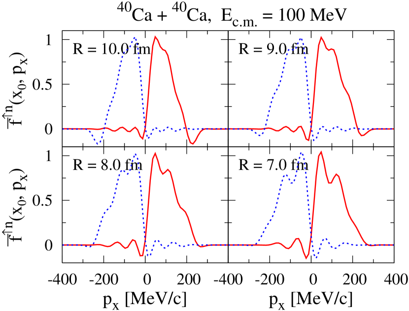
Figure 3: Reduced Wigner function ${\bar{f}}^{\uparrow n}(x_{0},p_{x})$ averaged over phase space on the window ($x=x_{0}$) for projectile-like (solid line) and target-like (dotted line) nuclei for the ⁴⁰Ca${}+^{40}$Ca reaction at $E_{\rm c.m.}=100$ MeV at different $R$. The Fermi momentum $p_{F}$ is taken as 270 MeV/$c$.

Examples of reduced Wigner function are shown in Fig. 3 for different relative distances. Not surprisingly, the reduced Wigner function is sometimes above 1 or below 0. This is indeed expected since the full quantum Wigner transform is considered without making use of any semiclassical approximation.

IV MOMENTUM DIFFUSION COEFFICIENT

In a recent work Washiyama1 , considering simple one-dimensional macroscopic reduction of TDHF, average transport properties of relative motion in heavy-ion collisions have been investigated. Temporal evolution of average value of relative distance $R(t)=\overline{R^{\lambda}(t)}$ and average value of relative momentum $P(t)=\overline{P^{\lambda}(t)}$ are calculated for average mean-field trajectory determined by the TDHF wave functions. Relative motion of colliding ions were analyzed in the basis of a simple classical equation of motion,

$$\frac{d}{dt}P=-\frac{d}{dR}U(R)-\gamma(R)\dot{R}.$$ (18)

Knowing time evolution of $R(t)$ and $P(t)$, average collective properties, namely, nucleus-nucleus potential energy $U(R)$ and form factor of one-body friction coefficient $\gamma(R)$ are determined by inverting Eq. (18). In this work, we consider the same geometry of head-on collision of heavy-ions and extend the macroscopic reduction treatment by considering the SMF approach. We analyze the relative motion by employing a Langevin equation. The Langevin equation for the relative motion has the form,

$$\frac{d}{dt}P^{\lambda}=-\frac{d}{dR^{\lambda}}U(R^{\lambda})-\gamma(R^{\lambda})\dot{R}^{\lambda}+\xi_{P}^{\lambda}(t),$$ (19)

where $\xi_{P}^{\lambda}(t)$ is a Gaussian random force acting on the relative motion. Ignoring non-Markovian effects, the random force reduces to white noise specified by a correlation function,

$$\overline{\xi_{P}^{\lambda}(t)\xi_{P}^{\lambda}({t}^{\prime})}=2\delta(t-{t}^{\prime})D_{PP}(R).$$ (20)

Here $D_{PP}(R)$ denotes the momentum diffusion coefficient, which may depend on the mean value of the relative distance $R$.

In order to extract momentum diffusion coefficient, we calculate the rate of change of the relative momentum employing the SMF equations. The rate of change of relative momentum involves kinetic parts due to nucleon exchange between projectile and target, and also involves terms arising from potential energy. In the previous investigation Washiyama2 , it is observed that during evolution from the entrance channel until passing over the Coulomb barrier, one-body dissipation mechanism is strongly correlated with nucleon exchange between projectile-like and target-like nuclei. This behavior is similar to phenomenological nucleon exchange model and the window formula for energy dissipation Randrup2 ; Feldmeier . Therefore, in the equation for the rate of change of relative momentum, we consider only kinetic terms corresponding to momentum flow across the window, which can be conveniently expressed in terms of reduced Wigner distribution as

$$\frac{d}{dt}P^{\lambda}=-\int{\frac{dp_{x}}{2\pi\hbar}}\frac{p_{x}^{2}}{m}f^{\lambda}(x,p_{x},t)|_{x=x_{0}}+{\rm potential~{}terms}.$$

Small fluctuations of relative momentum are connected to small amplitude fluctuations in Wigner distribution. Ignoring contribution arising from potential terms, we have for small fluctuations of relative momentum

$$\frac{d}{dt}\delta P^{\lambda}\approx-\int{\frac{dp_{x}}{2\pi\hbar}}\frac{p_{x}^{2}}{m}\delta f^{\lambda}(x,p_{x},t)|_{x=x_{0}}=\xi_{P}^{\lambda}(t).$$ (22)

The right hand side in this expression acts as a random force for generating fluctuations in the relative momentum. Since $\delta f^{\lambda}(x,p_{x},t)$ is a Gaussian random quantity, the random force $\xi_{P}(t)$ is also Gaussian random, which is specified by a correlation function,

$$\overline{\xi_{P}^{\lambda}(t)\xi_{P}^{\lambda}({t}^{\prime})} = \int\!\!\!\int\frac{dp_{x}}{2\pi\hbar}\frac{d{p}^{\prime}_{x}}{2\pi\hbar}\frac{p_{x}^{2}}{m}\frac{{p^{\prime}}_{x}^{2}}{m}$$ (23)

$${}\times\overline{\delta f^{\lambda}(x,p_{x},t)\delta f^{\lambda}(x,{p}^{\prime}_{x},{t}^{\prime})}|_{x=x_{0}}.$$

Using the expression for the correlation function of the reduced Wigner distribution in Eq. (12), according to Eq. (20), the momentum diffusion coefficient is given by

$$D_{PP}(t)=\int\frac{dp_{x}}{2\pi\hbar}\frac{|p_{x}|}{m}\frac{p_{x}^{2}}{2}\Lambda^{+}(x_{0},p_{x},t).$$ (24)

From the SMF approach, we cannot directly derive an expression for the friction coefficient $\gamma(R)$. The reason is that we cannot associate the net momentum flow across the window, which is given by the first term on the right side of Eq. (IV), with dissipative force acting on the relative motion. However, from the expression (24) for diffusion coefficient and from the random walk mechanism of nucleon exchange Randrup2 ; Feldmeier , we can infer an expression for the friction coefficient. In the expression for diffusion coefficient, first and second terms correspond to nucleon flux from projectile to target and from target to projectile, respectively. Each nucleon transfer changes the relative momentum by an amount $p_{x}$ and increases the dispersion of the relative momentum by an amount $p_{x}^{2}$. Nucleon transfer in both direction increases dispersion of relative momentum, therefore diffusion coefficient is determined by total nucleon flux, i.e., sum of flux from projectile to target and from target to projectile. On the other hand, dissipation is determined by the net momentum flow through the window. Hence, the resultant dissipative force can be expressed as

$$F(t)=\int{\frac{dp_{x}}{2\pi\hbar}}\frac{|p_{x}|}{m}p_{x}\Lambda^{-}(x_{0},p_{x},t).$$ (25)

Then, it is possible to deduce from TDHF simulations the momentum diffusion coefficient $D_{PP}(t)=D_{PP}(R)$ and the friction force $F(t)$ as a function of relative distance. We note that these transport coefficients correspond to the phenomenological window formula arising from the nucleon exchange mechanism Feldmeier , and they are determined in terms of the average evolution specified by the TDHF.

Rather than calculating the dissipative force, it is more instructive to calculate the friction coefficient $\gamma(R)$. For this purpose, we assume that dissipative force is proportional to relative velocity, i.e., $F(t)=-\gamma(R)\dot{R}$, and consider the reduced friction coefficient $\beta(R)=\gamma(R)/\mu(R)$, where $\mu(R)$ denotes inertia associated with relative motion. Solid lines in Fig. 4 show the reduced friction coefficient as a function of $R$ for head-on collision of ⁴⁰Ca${}+^{40}$Ca at two different center-of-mass energies. For each energy, enlarged plot around the Coulomb barrier region is shown in the insert. In a recent work Washiyama2 , we extracted the reduced friction coefficient associated with relative motion employing a different reduction procedure, so-called Dissipative-Dynamics TDHF (DD-TDHF), which, in principle, incorporates dissipation due to both window and wall mechanisms. Dashed lines in Fig. 4 show the results of this reduction procedure. Good agreement is found between two different calculations above and close to the Coulomb barrier ($\sim 9.8$ fm). Below the Coulomb barrier, the DD-TDHF method is not reliable. However, the method based on the SMF provides a proper description of the one-body friction coefficient due to nucleon exchange mechanism for a wide range of relative distance.

Figure 4: Reduced friction coefficient $\beta(R)=\gamma(R)/\mu$ as a function of $R$ for the ⁴⁰Ca${}+^{40}$Ca reaction at $E_{\rm c.m.}=100$ MeV (upper panel) and at $E_{\rm c.m.}=150$ MeV (lower panel). For each energy, a zoom on the Coulomb barrier region is also shown in the insert.

Solid lines in Fig. 5 show the momentum diffusion coefficient $D_{PP}$, Eq. (24), as a function of $R$ for head-on collision of ⁴⁰Ca${}+^{40}$Ca at two different center-of-mass energies. Similarly to the reduced friction coefficient, magnitude of the momentum diffusion coefficient increases for decreasing relative distance. The increase of magnitude of transport coefficients, i.e., friction and diffusion coefficients, for decreasing $R$ is essentially due to larger window area and larger number of nucleon exchange between projectile-like and target-like nuclei. It is important to realize that, even though the ordinary TDHF does not contain information about density fluctuations, we can employ the average information provided by the TDHF to calculate diffusion coefficients associated with macroscopic variables. In practical applications, the momentum diffusion coefficient is usually taken as the thermal equilibrium value determined by the Einstein relation in terms of friction coefficient and effective temperature as

$$D^{\rm eq}_{PP}(R)=\gamma(R)T(t)$$ (26)

In this expression, $T(t)$ denotes the effective temperature assuming local equilibrium. It can be determined in terms of excitation energy denoted by $E^{*}$ by the relation $T(t)=\sqrt{E^{*}(t)/a}$, where $a$ denotes level density parameter, taken here as $a=A/12$. We can estimate the excitation energy in terms of dissipated energy according to

$$E^{*}(t)=\int_{0}^{t}dt^{\prime}\gamma[R(t^{\prime})][\dot{R}(t^{\prime})]^{2}$$ (27)

Dashed lines in Fig. 5 show the diffusion coefficient $D^{\rm eq}_{PP}(R)$ determined according to the Einstein relation. As seen from the figure, the Einstein relation severely underestimates magnitude of dynamical diffusion coefficient. The fact that the Einstein relation severely underestimates the dynamical diffusion coefficient associated with the relative motion was already realized in the phenomenological description of nucleon exchange model in Ref. Feldmeier .

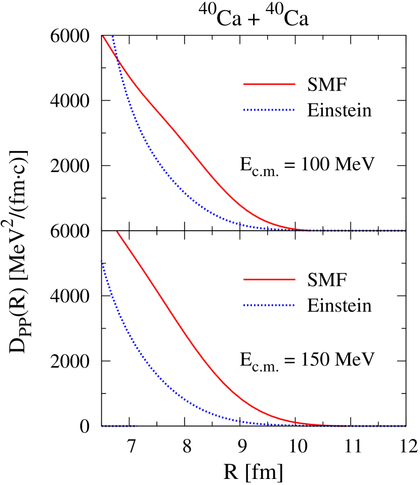
Figure 5: Diffusion coefficient $D_{PP}$ obtained by SMF (solid lines) and by the Einstein relation $D_{PP}^{\rm eq}=\gamma(R)T(t)$ (dashed lines) as a function of $R$ for the ⁴⁰Ca${}+^{40}$Ca reaction at $E_{\rm c.m.}=100$ MeV (upper panel) and at $E_{\rm c.m.}=150$ MeV (lower panel).

V CONCLUSIONS

Recently proposed stochastic mean-field theory incorporates both one-body dissipation and fluctuation mechanisms in a manner consistent with quantal fluctuation-dissipation theorem of non-equilibrium statistical mechanics Ayik2 . This was illustrated for slow collective motion by projecting equation of motion of the SMF onto a collective space in adiabatic limit. The projection gives rise to a generalized Langevin equation for collective variables, in which mean-field dissipation and fluctuation mechanisms are connected through the quantal fluctuation-dissipation relation. Therefore, this approach provides a powerful tool for microscopic description of low energy nuclear processes in which two-body dissipation and fluctuation mechanisms do not play important role. The low energy processes include induced fission, heavy-ion fusion near barrier energies, and spinodal decomposition during the expansion phase of hot piece of nuclear matter produced in heavy-ion collisions Ayik3 ; Maria .

In this work, we carry out a different projection of the SMF approach on the relative motion in fusion reaction by following the DD-TDHF method introduced in Washiyama1 and deduce one-body friction and one-body diffusion coefficients associated with relative motion. It is remarkable that expressions of transport coefficients for the relative motion (as well as transport coefficients for other macroscopic variables which are not mentioned in this work) have the same form as given by the phenomenological nucleon exchange model Randrup2 ; Feldmeier . The phenomenological nucleon exchange model involves an important assumption, namely, when a nucleon passes through the window, it instantaneously equilibrates with the new environment on the other side of the window. On the other hand, transport coefficients deduced from the SMF approach do not involves this assumption, and also they are not restricted by adiabatic or diabatic approximation. Therefore, these transport coefficients provide a microscopic basis for determining magnitude of the actual one-body dissipation and the corresponding mean-field fluctuation mechanism. We also stress the fact that, assuming amplitude of density fluctuations are small, transport coefficients are calculated in terms of the average evolution determined by TDHF simulations as a function of relative distance. In the continuation of the investigations, we plan to generalize the projection procedure of the SMF approach for off-central collisions and also deduce transport coefficients for nucleon diffusion in grazing heavy-ion collisions.

*

Appendix A CORRELATION FUNCTION OF WIGNER DISTRIBUTION

Small amplitude fluctuations of Wigner distribution can be expressed as

$$\delta f^{\lambda}(\bm{r},\bm{p},t)=\int d^{3}s\exp\left(-\frac{i}{\hbar}\bm{p}\cdot\bm{s}\right)$$

$${}\times\sum\limits_{ij\sigma\tau}\Phi_{j\sigma\tau}^{\ast}\left(\bm{r}+\frac{\bm{s}}{2},t\right)\delta\rho_{ij}^{\lambda}(\sigma\tau)\Phi_{i\sigma\tau}\left(\bm{r}-\frac{\bm{s}}{2},t\right),$$

where the single-particle wave functions are complete set of solutions of the ordinary TDHF. The initial values of stochastic expansion coefficients $\delta\rho_{ij}^{\lambda}(\sigma\tau)$ are Gaussian random numbers as specified by Eq. (II). In principle, these coefficients evolve in time according to time-dependent RPA equations. Here, we ignore this evolution and take them as Gaussian random numbers as specified by the initial conditions. Fluctuating part of the density matrix can be separated into four groups, $\delta\rho_{PP}^{\lambda}$, $\delta\rho_{TT}^{\lambda}$, $\delta\rho_{PT}^{\lambda}$ and $\delta\rho_{TP}^{\lambda}$, which are associated with wave functions originating from projectile and target nuclei and the mixed terms. As a result, small amplitude fluctuations of the Wigner distribution separate into four parts, $\delta f_{PP}^{\lambda}(\bm{r},\bm{p},t)$, $\delta f_{TT}^{\lambda}(\bm{r},\bm{p},t)$, $\delta f_{PT}^{\lambda}(\bm{r},\bm{p},t)$ and $\delta f_{TP}^{\lambda}(\bm{r},\bm{p},t)$. We calculate the equal time correlation function of the Wigner distribution in semi-classical approximation. First, we consider the correlation function associated with wave functions originating from projectile. Using the expression (II) for the variance of the matrix elements, we deduce

$$\overline{\delta f_{PP}^{\lambda}(\bm{r},\bm{p},t)\delta f_{PP}^{\lambda}({\bm{r}}^{\prime},{\bm{p}}^{\prime},t)}=\int\!\!\!\int{d^{3}sd^{3}{s}^{\prime}\exp\left(-\frac{i}{\hbar}\bm{p}\cdot\bm{s}\right)}\exp\left(-\frac{i}{\hbar}{\bm{p}}^{\prime}\cdot{\bm{s}}^{\prime}\right)$$

$${}\times\sum\limits_{ij\sigma\tau\in P}{\Phi_{j\sigma\tau}^{\ast}\left(\bm{r}+\frac{\bm{s}}{2},t\right)}\Phi_{i\sigma\tau}\left(\bm{r}-\frac{\bm{s}}{2},t\right)\Phi_{i\sigma\tau}^{\ast}\left({\bm{r}}^{\prime}+\frac{{\bm{s}}^{\prime}}{2},t\right)\Phi_{j\sigma\tau}\left({\bm{r}}^{\prime}-\frac{{\bm{s}}^{\prime}}{2},t\right)n_{j}^{\sigma\tau}(1-n_{i}^{\sigma\tau}).$$ (29)

In the term that is proportional to $n_{j}^{\sigma\tau}$, we use the closure relations to find,

$$\sum\limits_{i\in P}{\Phi_{i\sigma\tau}^{\ast}\left({\bm{r}}^{\prime}+\frac{{\bm{s}}^{\prime}}{2},t\right)}\Phi_{i\sigma\tau}\left(\bm{r}-\frac{\bm{s}}{2},t\right)=\delta\left({\bm{r}}^{\prime}-\bm{r}+\frac{{\bm{s}}^{\prime}+\bm{s}}{2}\right).$$ (30)

In this expression, summation runs over a complete set of single-particle states, i.e., occupied and unoccupied states originating from the projectile. The closure relation satisfied by the complete set of states at the initial state will remain valid at later times. In the second step, we introduce the Wigner distribution,

$$\sum\limits_{j\in P}\Phi_{j\sigma\tau}^{\ast}\left(\bm{r}+\frac{\bm{s}}{2},t\right)n_{j}^{\sigma\tau}\Phi_{j\sigma\tau}\left({\bm{r}}^{\prime}-\frac{{\bm{s}}^{\prime}}{2},t\right)=\int\frac{d^{3}Q}{(2\pi\hbar)^{3}}\exp\left[\frac{i}{\hbar}\left(\bm{r}-{\bm{r}}^{\prime}+\frac{\bm{s}+{\bm{s}}^{\prime}}{2}\right)\cdot\bm{Q}\right]f_{P}^{\sigma\tau}\left(\frac{\bm{r}+{\bm{r}}^{\prime}}{2}+\frac{\bm{s}-{\bm{s}}^{\prime}}{4},\bm{Q},t\right),$$

where $f_{P}^{\sigma\tau}(\bm{r},\bm{p},t)$ denotes the ensemble averaged Wigner distribution associated with wave functions originating from projectile in spin-isospin channel $(\sigma,\tau)$. After making transformations, $\bm{s}={}+\bm{\eta}+\bm{Y}/2$ and ${\bm{s}}^{\prime}={}-\bm{\eta}+\bm{Y}/2$, the term that is proportional to occupation factor $n_{j}^{\sigma\tau}$ in the right-hand side of Eq. (A) becomes

$$\sum_{\sigma\tau}\int\!\!\!\int\!\!\!\int d^{3}Yd^{3}\eta\exp\left[-\frac{i}{\hbar}\left(\bm{Y}\cdot\frac{\bm{p}+{\bm{p}}^{\prime}}{2}\right)\right]\exp\left[-\frac{i}{\hbar}\bm{\eta}\cdot(\bm{p}-{\bm{p}}^{\prime})\right]$$ (32)

$${}\times\frac{d^{3}Q}{(2\pi\hbar)^{3}}\exp\left[\frac{i}{\hbar}\bm{Y}\cdot\bm{Q}\right]f_{P}^{\sigma\tau}\left(\bm{r}-\frac{\bm{Y}}{4}+\frac{\bm{\eta}}{2},\bm{Q},t\right)\delta\left({\bm{r}}^{\prime}-\bm{r}+\frac{\bm{Y}}{2}\right).$$

Assuming that the Wigner distribution is a smooth function of $\bm{r}$, $f_{P}^{\sigma\tau}(\bm{r}-\frac{\bm{Y}}{4}+\frac{\bm{\eta}}{2},\bm{Q},t)\approx f_{P}^{\sigma\tau}(\bm{r},\bm{Q},t)$ and $\delta({\bm{r}}^{\prime}-\bm{r}+\frac{\bm{Y}}{2})\approx\delta(\bm{r}-{\bm{r}}^{\prime})$, we can carry out the integrations over $\bm{\eta}$ and $\bm{Y}$ to obtain $(2\pi\hbar)^{3}\delta(\bm{p}-{\bm{p}}^{\prime})$ and $(2\pi\hbar)^{3}\delta(\bm{p}-\bm{Q})$, respectively. As a result, the term (32) becomes

$${\rm(A.5)}=(2\pi\hbar)^{3}\delta(\bm{p}-\bm{p}^{\prime})\delta(\bm{r}-{\bm{r}}^{\prime})\sum\limits_{\sigma\tau}f_{P}^{\sigma\tau}(\bm{r},\bm{p},t).$$ (33)

For the term proportional to $n_{i}^{\sigma\tau}n_{j}^{\sigma\tau}$ in Eq. (A), again we introduce the Wigner distribution for the factor involving the index $j$,

$$\sum\limits_{j\in P}\Phi_{j\sigma\tau}^{\ast}\left(\bm{r}+\frac{\bm{s}}{2}\right)n_{j}^{\sigma\tau}\Phi_{j\sigma\tau}\left({\bm{r}}^{\prime}-\frac{{\bm{s}}^{\prime}}{2}\right)=\int\frac{d^{3}Q_{1}}{(2\pi\hbar)^{3}}\exp\left[\frac{i}{\hbar}\left(\bm{r}-{\bm{r}}^{\prime}+\frac{\bm{s}+\bm{s}^{\prime}}{2}\right)\cdot\bm{Q}_{1}\right]f_{P}^{\sigma\tau}\left(\frac{\bm{r}+{\bm{r}}^{\prime}}{2}+\frac{\bm{s}-{\bm{s}}^{\prime}}{4},\bm{Q}_{1},t\right),$$

and for the one involving the index $i$,

$$\sum\limits_{i\in P}\Phi_{i\sigma\tau}^{\ast}\left({\bm{r}}^{\prime}+\frac{{\bm{s}}^{\prime}}{2}\right)n_{i}^{\sigma\tau}\Phi_{i\sigma\tau}\left(\bm{r}-\frac{\bm{s}}{2}\right)=\int\frac{d^{3}Q_{2}}{(2\pi\hbar)^{3}}\exp\left[\frac{i}{\hbar}\left({\bm{r}}^{\prime}-\bm{r}+\frac{\bm{s}+{\bm{s}}^{\prime}}{2}\right)\cdot\bm{Q}_{2}\right]f_{P}^{\sigma\tau}\left(\frac{\bm{r}+{\bm{r}}^{\prime}}{2}+\frac{{\bm{s}}^{\prime}-\bm{s}}{4},\bm{Q}_{2},t\right).$$

Making the same transformations, $\bm{s}=+\bm{\eta}+\bm{Y}/2$ and ${\bm{s}}^{\prime}=-\bm{\eta}+\bm{Y}/2$, the term that is proportional to $n_{i}^{\sigma\tau}n_{j}^{\sigma\tau}$ in the right-hand side of Eq. (A) becomes

$$\sum_{\sigma\tau}\int\!\!\!\int\!\!\!\int\!\!\!\int d^{3}Yd^{3}\eta\exp\left[-\frac{i}{\hbar}\left(\bm{Y}\cdot\frac{\bm{p}+{\bm{p}}^{\prime}}{2}\right)\right]\exp\left[-\frac{i}{\hbar}\bm{\eta}\cdot(\bm{p}-{\bm{p}}^{\prime})\right]\frac{d^{3}Q_{1}}{(2\pi\hbar)^{3}}\frac{d^{3}Q_{2}}{(2\pi\hbar)^{3}}\exp\left[\frac{i}{\hbar}\left(\bm{r}-{\bm{r}}^{\prime}+\frac{\bm{Y}}{2}\right)\cdot\bm{Q}_{1}\right]$$ (36)

$${}\times\exp\left[\frac{i}{\hbar}\left({\bm{r}}^{\prime}-\bm{r}+\frac{\bm{Y}}{2}\right)\cdot\bm{Q}_{2}\right]f_{P}^{\sigma\tau}\left(\frac{\bm{r}+{\bm{r}}^{\prime}}{2}+\frac{\bm{\eta}}{2},\bm{Q}_{1},t\right)f_{P}^{\sigma\tau}\left(\frac{\bm{r}+{\bm{r}}^{\prime}}{2}-\frac{\bm{\eta}}{2},\bm{Q}_{2},t\right).$$

We introduce another change of variables $\bm{Q}_{1}=\bm{Q}+\bm{q}/2$ and $\bm{Q}_{2}=\bm{Q}-\bm{q}/2$, and again assume that the Wigner distribution has a smooth function of $\bm{r}$ and ignore $\bm{\eta}$ dependence. Then, integrations over $\bm{\eta}$, $\bm{q}$ and $\bm{Y}$ give $(2\pi\hbar)^{3}\delta(\bm{p}-{\bm{p}}^{\prime})$, $(2\pi\hbar)^{3}\delta(\bm{r}-{\bm{r}}^{\prime})$ with $\bm{Q}_{1}\approx\bm{Q}_{2}=\bm{Q}$ and $(2\pi\hbar)^{3}\delta(\bm{p}-{\bm{Q}})$, respectively. As a result, the term (36) becomes

$${\rm(A.9)}=(2\pi\hbar)^{3}\delta(\bm{p}-{\bm{p}}^{\prime})\delta(\bm{r}-{\bm{r}}^{\prime})\sum\limits_{\sigma\tau}f_{P}^{\sigma\tau}(\bm{r},\bm{p},t)f_{P}^{\sigma\tau}(\bm{r},\bm{p},t).$$ (37)

Combining together, equal time correlation function (A) of the Wigner distribution associated with wave functions originating from projectile becomes,

$$\overline{\delta f_{PP}^{\lambda}(\bm{r},\bm{p},t)\delta f_{PP}^{\lambda}({\bm{r}}^{\prime},{\bm{p}}^{\prime},t)}=(2\pi\hbar)^{3}\delta(\bm{p}-{\bm{p}}^{\prime})\delta(\bm{r}-{\bm{r}}^{\prime})\sum\limits_{\sigma\tau}f_{P}^{\sigma\tau}(\bm{r},\bm{p},t)[1-f_{P}^{\sigma\tau}(\bm{r},\bm{p},t)].$$ (38)

In a similar manner, we can calculate the correlation function of the Wigner distribution associated with wave functions originating from target and from mixed configuration,

$$\overline{\delta f_{TT}^{\lambda}(\bm{r},\bm{p},t)\delta f_{TT}^{\lambda}({\bm{r}}^{\prime},{\bm{p}}^{\prime},t)}=(2\pi\hbar)^{3}\delta(\bm{p}-{\bm{p}}^{\prime})\delta(\bm{r}-{\bm{r}}^{\prime})\sum\limits_{\sigma\tau}f_{T}^{\sigma\tau}(\bm{r},\bm{p},t)\left[1-f_{T}^{\sigma\tau}(\bm{r},\bm{p},t)\right]$$ (39)

and

$$\overline{\delta f_{PT}^{\lambda}(\bm{r},\bm{p},t)\delta f_{PT}^{\lambda}({\bm{r}}^{\prime},{\bm{p}}^{\prime},t)}=(2\pi\hbar)^{3}\delta(\bm{p}-{\bm{p}}^{\prime})\delta(\bm{r}-{\bm{r}}^{\prime})\Lambda^{+}(\bm{r},\bm{p},t),$$ (40)

where

$$\Lambda^{+}(\bm{r},\bm{p},t)=\sum\limits_{\sigma\tau}\left\{f_{P}^{\sigma\tau}(\bm{r},\bm{p},t)\left[1-f_{T}^{\sigma\tau}(\bm{r},\bm{p},t)\right]+f_{T}^{\sigma\tau}(\bm{r},\bm{p},t)\left[1-f_{P}^{\sigma\tau}(\bm{r},\bm{p},t)\right]\right\}.$$ (41)

Total correlation function of the Wigner distribution is the sum of (38), (39) and (40). In the mean-field description, the sub-spaces of wave functions originating from projectile and target nuclei behave like pure states. Therefore, contributions of correlations coming from direct terms involving $f_{P}^{\sigma\tau}(\bm{r},\bm{p},t)\left[1-f_{P}^{\sigma\tau}(\bm{r},\bm{p},t)\right]$ and $f_{T}^{\sigma\tau}(\bm{r},\bm{p},t)\left[1-f_{T}^{\sigma\tau}(\bm{r},\bm{p},t)\right]$ are expected to be small. Hence, we can approximately express the total correlation function of Wigner distribution as,

$$\overline{\delta f^{\lambda}(\bm{r},\bm{p},t)\delta f^{\lambda}({\bm{r}}^{\prime},{\bm{p}}^{\prime},t)}\approx(2\pi\hbar)^{3}\delta(\bm{p}-{\bm{p}}^{\prime})\delta(\bm{r}-{\bm{r}}^{\prime})\Lambda^{+}(\bm{r},\bm{p},t).$$ (42)

We also want to calculate different time correlation function of the Wigner distribution. Assuming that the correlation function has short correlation time, i.e., much shorter than mean-free path, different time correlation function can be deduced by observing that in short time intervals of order of correlation time $|t-{t}^{\prime}|\leq\tau_{corr}$, Wigner distribution may be approximated as a free propagation, $\delta f(\bm{r},\bm{p},t+\tau)\approx\delta f(\bm{r}-\tau\bm{p}/m,\bm{p},t)$. As a result, different time correlation function can be expressed as,

$$\overline{\delta f^{\lambda}(\bm{r},\bm{p},t)\delta f^{\lambda}({\bm{r}}^{\prime},{\bm{p}}^{\prime},{t}^{\prime})}=(2\pi\hbar)^{3}\delta(\bm{p}-{\bm{p}}^{\prime})\delta\left[\bm{r}-{\bm{r}}^{\prime}-(t-{t}^{\prime})\bm{p}/m\right]\Lambda^{+}(\bm{r},\bm{p},t).$$ (43)

In order to deduce the correlation function on the window, $x={x}^{\prime}=x_{0}$, we notice that

$$\delta\left[\bm{r}-{\bm{r}}^{\prime}-(t-{t}^{\prime})\bm{p}/m\right]\to\frac{m}{|p_{x}|}\delta(t-{t}^{\prime})\delta(y-{y}^{\prime})\delta(z-{z}^{\prime}).$$ (44)

In determining transport coefficients, we need to carry out integration over window variables, $y,z,p_{y},p_{z}$, of product of Wigner distributions. Since construction of three-dimensional Wigner functions in terms of TDHF wave functions requires a large numerical effort, we introduce the following approximation for the phase-space integration over the window,

$$\int\!\!\!\int{dydz\frac{dp_{y}dp_{z}}{(2\pi\hbar)^{2}}}f_{P}^{\sigma\tau}(\bm{r},\bm{p},t)f_{T}^{\sigma\tau}(\bm{r},\bm{p},t)\approx\frac{1}{\Omega(x,t)}f_{P}^{\sigma\tau}(x,p_{x},t)f_{T}^{\sigma\tau}(x,p_{x},t).$$ (45)

Here $\Omega(x,t)$ denotes the phase-space volume on the window. As a result, the correlation function on the window can be expressed in terms of the reduced Wigner distributions along $x$-axis given by Eq. (12).

References

- (1) P. Ring and P. Schuck, The Nuclear Many-Body Problem,Springer, New York, 1980.
- (2) K. Goeke and P.-G. Reinhard, Time-Dependent Hartree-Fock and Beyond, Bad Honnef, Germany, 1982.
- (3) K.T.D. Davis, K. R. S. Devi, S. E. Koonin and M. Strayer, Treatise in Heavy-Ion Science, ed. D. A. Bromley, Nuclear Science V-4, Plenum, New York, 1984
- (4) C. Simenel, B. Avez and D. Lacroix, Lecture notes of the ”International Joliot-Curie School”, Maubuisson, September 17-22, 2007, arXiv:0806.2714.
- (5) S. E. Koonin, Prog. Part. Nucl. Phys. 4, 283 (1980).
- (6) J. W. Negele, Rev. Mod. Phys. 54, 913 (1982).
- (7) C. W. Gardiner, Quantum Noise, Springer-Verlag, Berlin, 1991.
- (8) U. Weiss, Quantum Dissipative Systems, World Scientific, Singapore, 1999.
- (9) S. Ayik and C. Gregoire, Phys. Lett. B212, 269 (1988); Nucl. Phys. A513, 187 (1990).
- (10) J. Randrup and B. Remaud, Nucl. Phys. A514, 339 (1990).
- (11) Y. Abe, S. Ayik, P.-G. Reinhard, and E. Suraud, Phys. Rep. 275, 49 (1996).
- (12) D. Lacroix, S. Ayik and Ph. Chomaz, Prog. Part. Nucl. Phys. 52, 497 (2004).
- (13) C. H. Dasso, Proc. Second La Rapida Summer School on Nuclear Physics, eds. M. Lozano and G. Madurga, World Scientific, Singapore, 1985.
- (14) C. H. Dasso and R. Donangelo, Phys. Lett. B276, 1 (1992).
- (15) S. Ayik, Phys. Lett. B658, 174 (2008).
- (16) S. Ayik, N. Er, O. Yilmaz and A. Gokalp, Nucl. Phys. A812, 44 (2008).
- (17) R. Balian, M. Veneroni, Phys. Lett. B136, (1984).
- (18) H. Mori, Prog. Theor. Phys. 33, 423 (1965).
- (19) K. Washiyama and D. Lacroix, Phys. Rev. C 78, 024610 (2008).
- (20) A. S. Umar and V. E. Oberacker, Phys. Rev. C 74, 061601(R) (2006); 76, 014614 (2007).
- (21) K. Washiyama, D. Lacroix and S. Ayik, submitted to Phys. Rev. C., arXiv:0811.4130.
- (22) K.-H. Kim, T. Otsuka, and P. Bonche, J. Phys. G 23, 1267 (1997).
- (23) J. Randrup and W. J. Swiatecki, Ann. Phys. (N.Y.) 125, 193 (1980); Nucl. Phys. A429, 105 (1984).
- (24) H. Feldmeier, Rep. Prog. Phys. 50, 915 (1987).
- (25) M. Colonna, Ph. Chomaz and S. Ayik, Phys. Rev. Lett. 88, 122701 (2002).