Cumulants of the current in the weakly asymmetric exclusion process
Abstract
We study the fluctuations of the total current for the partially asymmetric exclusion process in the scaling of a weak asymmetry (asymmetry of order the inverse of the size of the system) using Bethe Ansatz. Starting from the functional formulation of the Bethe equations, we obtain for all the cumulants of the current both the leading and next-to-leading contribution in the size of the system.
pacs:
05-40.-a; 05-60.-kI Introduction
The one dimensional asymmetric simple exclusion process (ASEP) is one of the most simple examples of a classical interacting particles system exhibiting a non equilibrium steady state. This stochastic system has been studied much in the past, both in the mathematical S70.1 ; L85.1 ; F08.1 and physical literature KLS84.1 ; S91.1 ; HHZ95.1 ; SZ95.1 ; D98.1 ; S01.1 ; GM06.1 ; D07.1 . It consists of particles hopping locally on a one dimensional lattice, with an asymmetry between the forward and backward hopping rates. The exclusion constraint prevents the particles from moving to a site already occupied by another particle. The asymmetry between the hopping rates models the action of an external driving field in the bulk of the system, which maintains a permanent macroscopic current in the system. This current breaks the detailed balance and keeps the system out of equilibrium even in the stationary state. The special case for which the particles hop forward and backward with equal rates is called the symmetric simple exclusion process (SSEP). It corresponds to a situation for which the detailed balance holds in the bulk which means (in the absence of boundary conditions breaking the forward-backward symmetry) that the system reaches equilibrium in the long time limit. In this case, the system belongs to the universality class of the Edwards–Wilkinson (EW) equation EW82.1 ; HHZ95.1 . On the contrary, if the two hopping rates are different, detailed balance is broken and the system reaches in the long time limit a non equilibrium steady state characterized by the presence of a current of particles flowing through the system. In that case, the system belongs to the universality class of the Kardar–Parisi–Zhang (KPZ) equation KPZ86.1 ; HHZ95.1 .
Because of its simplicity, the ASEP is an interesting tool to investigate the general properties of systems out of equilibrium. Moreover, the ASEP is related through various mappings to many other models, in particular: the zero range process EH05.1 , directed polymers in a random medium K97.1 , interface growth models GS92.1 ; HHZ95.1 ; K97.1 , the six vertex model KDN90.1 ; GS92.1 , XXZ spin chains GS92.1 ; ER96.1 ; GM06.1 . It is also used as a starting point to model physical phenomena such as cellular molecular motors LKN01.1 , hopping conductivity R77.1 , traffic flow CSS00.1 , usually by enriching the dynamics of the ASEP by new rules that makes it closer to the studied phenomenon.
The ASEP, along with a very small number of other statistical mechanics models is known to be “exactly solvable” in the sense that several quantities can be calculated exactly, which is a rather uncommon property. The totally asymmetric case, for which all the particles hop in only one direction (TASEP), is usually the easiest to solve. On the contrary, the model with partial asymmetry often exhibits a more intricate mathematical structure and is thus more difficult to solve. A few different approaches have been used in the past to obtain exact results for the ASEP: the matrix product representation DEHP93.1 ; BE07.1 allows to calculate explicitly the probabilities of all the configurations in the stationary state for both open systems connected to reservoirs of particles and systems on a ring with periodic boundary conditions; techniques from random matrix theory PS02.1 ; S06.1 ; S07.1 have been used for the study of infinite systems defined on ; Bethe Ansatz has provided many exact results, principally on a ring D87.1 ; GS92.1 , but also recently for open systems dGE05.1 .
The fact that Bethe Ansatz can be used to study the ASEP is strongly related to the “quantum integrability” of the model. Indeed, the Markov matrix governing the time evolution of the probabilities for the configurations of the ASEP is similar to the hamiltonian of the XXZ spin chain and closely related to the transfer matrix of the six vertex model. While its formulation for the ASEP is well understood, the use of the Bethe Ansatz is usually quite technical. The difficulty lies in the determination of the so called “Bethe roots” in terms of which all the quantities we want to calculate are expressed. These Bethe roots are solutions of a set of highly coupled polynomial equations called the Bethe equations of the system. Their solutions are usually not known for general values of the parameters of the model studied. In the case of the ASEP, Bethe Ansatz has been used successfully to calculate the gap of the system GS92.1 ; K95.1 ; GM04.1 ; dGE05.1 ; dGE08.1 , related to the dynamical exponent which governs the speed at which the system reaches its stationary state. It has also allowed to calculate some properties of the fluctuations of the current in the stationary state DL98.1 ; DA99.1 ; LK99.1 ; DE99.1 ; ADLvW08.1 ; PM08.1 ; P08.1 .
In the present work, we study the fluctuations of the steady state current for the ASEP on a ring in the scaling of a weak asymmetry between the hopping rates (asymmetry scaling as the inverse of the size of the system). The main result of the article is the Bethe Ansatz derivation of all the cumulants of the current in this scaling limit. We obtain an explicit expression (9) for the leading and next-to-leading contributions in the size of the system. We use a rewriting of the Bethe equations for the ASEP in terms of a polynomial functional equation. Our approach is based on the functional Bethe Ansatz and does not rely on the behavior of the Bethe roots in the large system size limit. We check our results numerically by solving the functional Bethe equation for systems up to size .
In section II, we discuss our formula (9) for the cumulants of the current in the scaling of a weak asymmetry. In section III, we write the Bethe equations for the ASEP as a polynomial functional equation and recall how this equation can be solved perturbatively to calculate the first cumulants of the current. In section IV, we define a new version of the functional equation that remains regular in the symmetric limit. Then, in section V, we take the weakly asymmetric limit of this equation, and we solve it in section VI. A few technical calculations are relegated to the appendix.
II Cumulants of the current in the weakly asymmetric exclusion process
We consider the partially asymmetric simple exclusion process (PASEP) on a ring. It is a stochastic process involving classical hard core particles hopping on a one dimensional lattice with periodic boundary conditions. Each one of the sites can be occupied by at most one of the particles. The system evolves with the following local dynamics: in an infinitesimal time interval , each particle hops forward with probability and backward with probability if the destination site is empty (exclusion rule).
II.1 Fluctuations of the total current
We define the total integrated current between time and time as the total distance covered by all the particles in this duration. This is a random variable which depends on the trajectories of the particles starting in some configuration at time and evolving by the markovian dynamics up to time . We are interested in the fluctuations of in the long time limit, when the (finite size) system reaches its unique stationary state which is independent of the initial configuration . We emphasize that we consider here the long time limit for finite systems. We will take the large system size limit only in the end. This is a completely different regime from taking the infinite system size limit first and studying then the stationary state HHZ95.1 . We want to calculate the first cumulants of the current with respect to the stationary state probability distribution of , that is its mean value , the diffusion constant and the higher cumulants:
| (1) | |||
| (2) | |||
| (3) |
The characteristic function, defined as the mean value of behaves in the long time limit as PM08.1
| (4) |
where is the “fugacity” corresponding to the variable . Taking the derivatives of the previous expression with respect to , we see that is the exponential generating function of the cumulants of the current in the stationary state, i.e.
| (5) |
The generating function of the cumulants can be related to the large deviation function of the current . The function is defined from the asymptotic behavior of the probability distribution of as
| (6) |
The large deviation function of the current is equal to for and is strictly positive otherwise, leading to an exponentially vanishing probability in the long time limit except when is equal to the mean value of the current. Writing
| (7) |
we observe that is the Legendre transform of the large deviations function , that is
| (8) |
II.2 Cumulants of the current in the scaling of a weak asymmetry
The principal result of this article is the calculation of all the cumulants of the stationary state current in the weakly asymmetric scaling limit , or equivalently, the Taylor expansion in the vicinity of of the generating function . Using Bethe Ansatz, we find
| (9) | ||||
In this expression, is the particle density and the function is given by
| (10) |
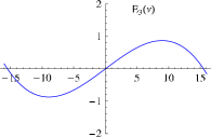
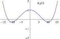
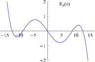
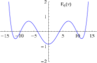
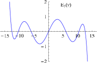
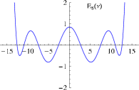
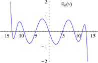
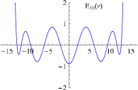
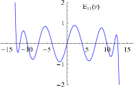
where the are the Bernoulli numbers. The expression (9) gives the leading and next-to-leading order in of all the cumulants of the current by taking the derivative with respect to . Only the subleading term of (9) contributes to the -th cumulant for . In this case, is a polynomial of degree in the rescaled asymmetry . The coefficients of this polynomial are expressed in terms of the Bernoulli numbers multiplied by factorials. The first cumulants are plotted with respect to the rescaled asymmetry in fig. 1. We note that they show oscillations in the parameter . This oscillation phenomenon of the cumulants of the current has been observed recently in the context of electron transport through a quantum dot in FFHNNBH09.1 . The special case which corresponds to the SSEP has already been calculated by Bethe Ansatz in ADLvW08.1 . For arbitrary , equation (9) leads to an expression for the large deviation function up to the order in , which matches the result obtained in ADLvW08.1 using the macroscopic fluctuation theory developed in BDSGJLL01.1 ; BDSGJLL04.1 .
|
 |
 |
||
|
 |
 |
||
|
 |
 |
We now justify the weakly asymmetric scaling chosen in equation (9). The crossover between the Edwards–Wilkinson and the Kardar–Parisi–Zhang behavior lies at a scaling where the asymmetry is nonzero but goes to zero when the size of the system goes to infinity. Consider a tagged particle in the system with asymmetry scaling as . During a time interval , this particle makes a number of rotations through the system. A typical time interval to consider is the time necessary for the system to reach its stationary state: , being the dynamic exponent of the system. Then, a criterion for separation between weak and strong asymmetry is when : when , the system is asymmetric, while corresponds to a symmetric system. This leads to . The value of depends on whether the system is in the Edwards–Wilkinson (EW, ) or in the Kardar–Parisi–Zhang (KPZ, ) universality class. This leads to two natural scalings for the asymmetry, and . It turns out that both of these scalings are meaningful for the ASEP. The scaling corresponds to the weakly asymmetric exclusion process, whereas the scaling corresponds to the crossover between the EW and the KPZ regimes K95.1 . In particular, the weakly asymmetric scaling belongs to the EW class like the symmetric exclusion process.
From the formula (9), we observe that for is a rather minimal deformation of the case . This modification is in fact needed to ensure that stays invariant under the Gallavotti–Cohen symmetry given by LS99.1 ; GM06.1
| (11) |
which in the weakly asymmetric scaling leads to
| (12) |
for the leading and next-to-leading order. The study of the exact values for the diffusion constant DM97.1 ; PM08.1 and the third cumulant P08.1 shows that these two cumulants are still given by equation (9) as long as . This suggests that this minimal deformation is valid in all the Edwards–Wilkinson universality class.
II.3 Phase transition
In BD05.1 , using the macroscopic fluctuation theory for driven diffusive systems developed in BDSGJLL01.1 ; BDSGJLL04.1 , the existence of a nontrivial dynamical phase transition was found in the weakly asymmetric exclusion process, with in particular a phase of weaker asymmetry for which the fluctuations of the current are gaussian (at dominant order in ), and a phase of stronger asymmetry in which the fluctuations of the current become non gaussian. Let be the value of the rescaled asymmetry corresponding to the separation between the gaussian and non gaussian phases. For , the large deviation function of the current (respectively the generating function of the cumulants of the current ) is quadratic in (resp. ) at the leading order in the size of the system. Performing the Legendre transform of the leading order of the expression (9) for , we find that in the gaussian phase , the large deviation function is given by the quadratic function of :
| (13) |
with
| (14) | ||||
| (15) |
at the leading order in . On the contrary, in the non gaussian phase , neither nor are expected to be quadratic, even at the leading order in . We emphasize that it does not contradict the fact that the Taylor expansion of given in equation (9) is quadratic in at the leading order. It merely means that the large limit of the asymptotic formula for breaks down and does not represent the full function anymore. We will come back to this issue at the end of this subsection.
According to BD05.1 , the density profile adopted by the system is dependent on the value of the current flowing through the system. In the gaussian phase, the density profile remains flat for all values of the current. In the non gaussian phase however, the density profile depends on the value of the current: there is a critical value for the current such that if , the density profile remains flat, while if , the profile becomes time dependent. The signature of this transition between the flat profile and the time dependent profile is visible through the appearance of non analyticities in the large deviation function of the current or, equivalently, in its Legendre transform, the (rescaled) generating function of the cumulants . A non analyticity in the large deviation function at corresponds to a non analyticity in at and related through the Gallavotti–Cohen symmetry as .
We now look at the non analyticities of the expression (9) for . From the asymptotic behavior of the Bernoulli numbers
| (16) |
we observe that has a singularity at . It corresponds for the function to singularities at the points . This equation has real solutions for if . Thus, non analyticities appears in as soon as for
| (17) |
and in this case, the non analyticities of are at the points
| (18) |
These expressions for and should hold only in the vicinity of since we used the expression (9) for which is valid for far from only in the gaussian phase. For the Legendre transform of the gaussian leading order of (9), we define the function such that
| (19) |
By the inverse function of , the values and correspond for the large deviation function to with
| (20) |
near . By Legendre transform, the function sends the region (where the density profile is time dependent) of the plane to the region , or equivalently , of the plane . It gives at the leading order of (9)
| (21) |
which agrees with equation (25) of BD05.1 (where is taken to be equal to ).
|
 |
|
|
 |
|
|
Our resolution of the functional Bethe equation of the ASEP (22) in the weakly asymmetric scaling limit, leading to the expression (9) for the cumulants of the current, relies on a perturbative expansion near of the functional Bethe equation. This approach does not always give an information on the value of for far from .
From the discussion in the beginning of this subsection of the gaussian/non-gaussian phase transition, it is expected that the function will be equal to its Taylor expansion for . In particular, the function should be quadratic in in the large limit. On the contrary, for , is expected to be different from its Taylor expansion (9), even at the leading order in .
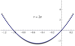
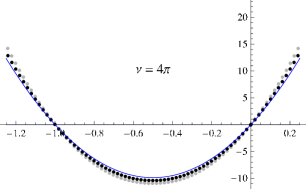
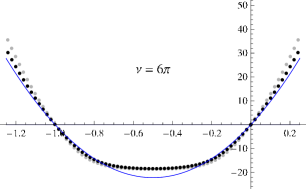
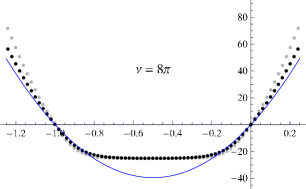
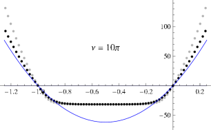
In order to check whether the function was equal to its Taylor expansion in given by (9), we studied numerically the Bethe equations of the ASEP for systems up to size (see appendix A). In fig. 2, we show the results we obtained at half filling () for different values of the asymmetry and of the size of the system . These results are in excellent agreement with the emergence of non gaussianity for : for , the numerical evaluation of fits well with the quadratic expression given by the leading order of equation (9). For , however, there is a region between and its symmetric by the Gallavotti–Cohen symmetry where differs significantly from the quadratic leading order of (9). Outside of this region, the numerical evaluation of still agrees with (9).
We emphasize that the fact is defined for a finite system in (5) and (9) as a generating function in , that is, as a Taylor series for at , does not contradict the fact that can be different from its Taylor expansion at in the large limit. An example of such a behavior is exhibited by the function . This function of and is, for finite , a rational fraction in which is entirely defined for by its Taylor expansion in through an analytic continuation, but develops an essential singularity in when .
III Reminder of the functional formulation of the Bethe equations
In this section, we recall the functional formulation of the Bethe Ansatz for the ASEP. We show how the generating function of the cumulants (5) can be expressed in terms of a solution to a functional polynomial equation and how this functional equation can be solved perturbatively to obtain the first cumulants.
It can be shown DL98.1 ; PM08.1 that the generating function of the cumulants of over the variable is equal to the eigenvalue with largest real part of a deformation of the Markov matrix of the system. Because of the underlying integrability of the ASEP, the diagonalization of can be performed using the Bethe Ansatz. The Bethe equations of the system can be rewritten PM08.1 in the functional equation
| (22) |
The polynomial is of degree and the polynomial is of degree . We choose the normalization of such that the coefficient of highest degree of is equal to one:
| (23) |
If we set in the functional Bethe equation (22), we obtain
| (24) |
which is the usual form of the Bethe equations in terms of the Bethe roots . Equations (22) and (24) are completely equivalent forms of the Bethe equations. In particular, they both have a large discrete set of solutions corresponding to the different eigenstates of the deformed matrix . We are only interested in the solution corresponding to the largest eigenvalue of , which is characterized by
| (25) |
Equivalently, the Bethe roots all tend to when for this solution of the Bethe equations. In the following, we will also use a relation coming from the fact that the stationary state is a zero momentum state PM08.1 . This condition implies
| (26) |
The generating function of the cumulants of the current is then given by PM08.1
| (27) |
In the rest of this section, we explain how the functional Bethe equation can be solved perturbatively near . Introducing the function
| (28) |
the functional Bethe equation (22) becomes
| (29) |
Note that we have added an extra factor in the definition compared to P08.1 . In terms of , equations (25), (26) and (27) become respectively
| (30) | ||||
| (31) | ||||
| (32) |
In the following, we will also need a few other properties of . Because is a polynomial of degree , we infer from the definition (28) of that
| (33) |
This equation fixes the term of highest degree of the polynomial , using the relation (29) between and :
| (34) |
Since the value of is known when is equal to zero (30), it is natural to attempt solving the functional Bethe equation (29) perturbatively near . Moreover, a perturbative solution of (29) in powers of gives access to the first cumulants of the current. Using (30), we write the expansion of in powers of as
| (35) |
From (25) and the definition (28) of , we deduce that the are polynomials in of degree . This observation will be crucial for the following. We will now see that equation (29) can be reformulated as a recurrence formula which can be used to calculate explicitly the first and, as a consequence, the first cumulants. In particular, the three first cumulants were calculated in P08.1 for finite size systems by this method that we now recall (see P08.1 for more details). Reminding that is a polynomial in , that is has only nonnegative powers in , we can eliminate it from equation (29) by doing the expansion for . We have
| (36) |
This equation must be understood in the following way: first, we expand the l.h.s. around in terms of the . Then, at each order in , the l.h.s. has a finite limit when , that is all the negative powers in from the cancel out. It is crucial to respect the order between the two expansions in and . Expanding first around makes the poles of (that is, the Bethe roots ) disappear from the problem, leaving us only with the algebraic properties of the polynomials . On the contrary, if we did the expansion in first, equation (36) would not contain any information since is regular when . Introducing the operator which acts on an arbitrary function as
| (37) |
we rewrite the previous equation in the slightly more complicated form
| (38) |
At order in , the r.h.s. depends only on the for . We emphasize that cancels out. This observation is the key that allows us to solve order by order in . Noting that acts separately on each power of and that , we can invert in (38). We have
| (39) |
The additional term comes from the fact that the operator gives when applied on . Recalling (33) and the fact that the have only negative (or zero) powers in , we finally obtain
| (40) |
We used the notation for the negative powers in of a function in its expansion near , after the perturbative expansion near as before. The constant can be set, order by order in , by the value (31) of . We note that in equation (40), , which was initially the size of the system and the degree of the polynomial , no longer needs being an integer. It can assume any complex value such that there is a constant which solves , that is for which the coefficient of in equation (40) is nonzero when . Thus, must be such that
| (41) |
We find that (31) can not be ensured if is an integer between and , which never happens for the ASEP because of the exclusion rule.
We note that the recurrence (40) is singular when since goes to in this limit. More precisely, starting from (30), the recurrence equation (40) gives for an expression which is regular when , as is applied on an a constant independent of at this order. Using again (40) to calculate , we see that the contributes a pole of order in . Iterating (40), we thus see that the have a pole of order in . As we are interested here in a scaling limit for which goes to as the size of the system goes to infinity, this form of the perturbative solution will not be usable. We have to transform it to make it suitable for the weakly asymmetric scaling limit.
IV Regularization of the functional equation
In this section, we regularize the function in the limit and show that the regularized function can be calculated perturbatively, in a similar way to what we did for in a previous section.
Equations (31) and (32) indicate that is regular in and that has only a pole of order in . But we also know that at order in the function has a pole of order in . This suggests that an expansion in should allow us to regularize the functional equation (29) in the limit . We define
| (42) |
In appendix B, we argue that is regular when and work out explicitly how the cancellation of divergent terms in works in the case of a system with only one particle. In the rest of this section, we will write a recurrence equation for similar to (40) for but regular in the limit . This will allow us to study the weakly asymmetric scaling limit. A difference will be that we will now have to do expansion both in and .
IV.1 Recurrence equation for
In terms of , the functional Bethe equation (29) rewrites
| (43) |
while equations (30), (31) and (32) become respectively
| (44) | ||||
| (45) | ||||
| (46) |
We will now solve the functional equation (43) perturbatively near and . We first write the expansion of near and as
| (47) |
The range for the summation over comes from (44) while the range for the summation over is a consequence of the regularity in of . Since the are polynomials (of degree ) in , we see that has only positive integer powers in after the expansion near and . A crucial point in the following will be that the are in fact polynomials in of degree , as can be seen writing at order in in the following way:
| (48) |
We used the fact that the have a pole of order in . We will now eliminate the polynomial from the functional equation (43) in a similar way to what we did in the previous section for the functional equation (29). We divide the functional equation (43) by and make the expansion . Taking (34) into account, we obtain
| (49) |
which must be understood as: each term of the expansion in power series in and of the l.h.s. is of order when . Once again, we see that the polynomial has disappeared, leaving us with an equation involving only . Replacing by and dividing everything by , equation (49) can be rewritten in the slightly more complicated form
| (50) |
Defining the finite difference operator acting on an arbitrary function as
| (51) |
the functional equation (50) finally becomes
| (52) |
with
| (53) |
and
| (54) |
Similarly to what happened in the recurrence equation (38) for , at order in and in , the r.h.s. of (52) depends only on the with either and () or and (). Thus, equation (52) provides a solution order by order in and of .
IV.2 Inversion of the operator
We see that contrary to what happened in (38), the operator acting on in the l.h.s. of (52) does not vanish when . This is related to the fact that that is not singular in the limit . The operator acts formally as
| (55) |
Using the Taylor expansion
| (56) |
where the are the Bernoulli numbers, we see that we can invert the operator in (52) by multiplying both sides by . We obtain
| (57) |
The differential operators and must be understood as the formal series (56) in . We now define some notations that will be useful in the following. For any function , we write the series expansion of when as
| (58) |
where is a (possibly negative) integer. We will note the singular part of when and the non-singular part of when , that is
| (59) |
and
| (60) |
When the function depends also on or , we define and such that all the expansions in powers of when goes to infinity must be done after the expansion in powers of and . Using (47), we can expand and near and . Since the are polynomials in , we see that at each order in and , and are also polynomials in . We can write
| (61) |
With these notations, we integrate equation (57) as a formal series in and only keep the divergent powers when (that is, the strictly positive powers in ). Taking (45) into account, we obtain
| (62) |
We did not add a constant term when doing the integration. This can be understood using the analytic continuation for complex in our formulas: since the are polynomials in , they have only positive integer powers in . But adding a constant term when integrating (57) would contribute a to . This is not possible as we have seen previously that we could take for any complex value. Using (56), we rewrite (62) as
| (63) |
After calculating the integral and using , we find
| (64) |
We observe that the denominator in this equation makes the previous equation divergent if is taken to be an integer. Thus, equation (64) must be understood by an analytic continuation in . The binomial coefficient in (64) is thus a polynomial of degree in . For , we see that the denominator cancels with the binomial coefficient, giving non singular terms in the limit where becomes an integer. For though, the denominator does not cancel with the binomial coefficient. It seems to make it impossible to have a finite limit for the r.h.s. of equation (64) when tends to an integer. But, as we know that is analytic in provided that , it simply means that the numerator contains factors canceling the non-analyticities in integer larger than . This is indeed shown by using the fact that the are polynomials in of degree . From the definitions (53) and (54), this implies that and are polynomials of degree at order in and in . Thus, only the terms with contribute to in equation (64). If we choose and such that , we will only need the terms of the sum over such that . We observe that for these terms, the denominator is always nonzero, even for integer. Thus, using the notation
| (65) |
we can rewrite (64) as
| (66) |
In this last equation, we can take to be an integer: there are no divergences anymore.
V Recurrence relations in the weakly asymmetric scaling limit
In this section, we take the weakly asymmetric limit (, ) of the recurrence relation (66) for . We write closed equations verified by the leading and next-to-leading expressions in the size of the system of a rescaled version of .
From the expression (54) for , we see that we will have to take of order in order to obtain a non trivial expression at finite density . It is useful to consider the function
| (67) |
From now on, we will no longer use the variables and . All the expansions in powers of and will be replaced with expansions in powers of the rescaled variables and . Recalling the fact that the are polynomials in of degree , we obtain from (47) that is of order when the size of the system goes to infinity. We write
| (68) |
Equations (44) and (45) become
| (69) | ||||
| (70) |
while from (46), the rescaled generating function of the cumulants of the current is given in terms of the function by
| (71) |
The binomial coefficient appearing in (66) has the expansion
| (72) |
where is equal to if and otherwise. Inserting (72) in (66), the recurrence becomes
| (73) |
Using (56) to perform the summation over , we find
| (74) |
We can finally perform the summation over and we obtain
| (75) | ||||
We recall that, from (53), (54) and (67), and are well defined functions depending on only through . Equation (75) is thus a closed equation verified by . It will allow us to obtain both the leading () and next-to-leading () terms of in the size of the system. We now have to expand both and to order two in to obtain an equation for and an equation for . The definition of (53) gives
| (76) |
with
| (77) | ||||
where is the particle density. Similarly, using the definition of (54), we find
| (78) |
where we have defined
| (79) |
and
| (80) | ||||
From (V) and (V), equation (75) gives at the leading order in the following closed equation for :
| (81) |
In the next section, we will solve this equation to find and thus the leading order of the rescaled generating function of the cumulants of the current. At the next-to-leading order , equation (75) leads to
| (82) |
with
| (83) |
and
| (84) | ||||
We used the fact that since (70). Once we know by solving equation (81), equation (82) becomes a closed equation for .
VI Solution of the weakly asymmetric functional relations
In this section, we explicitly solve the functional relations (81) and (82) to all order in and . We obtain the leading and the next-to-leading order in of the rescaled generating function .
VI.1 Leading order
Inserting the expressions (V), (79) and (V) for and , and using , the equation (81) for the leading order becomes
| (85) |
Multiplying both sides of the previous equation by , we obtain
| (86) |
Let us write the unknown function as
| (87) |
We can state (86) as an equation for . We obtain
| (88) |
Because of (70), we also want to have only strictly positive powers in order by order in and . This can be expressed in the form
| (89) |
In terms of , it becomes
| (90) |
We prove in appendix C that
| (91) |
is the unique formal power series in and that solves (88) and (90). Thus, equation (87) for with defined by (91) is the unique solution of (81).
VI.2 Next-to-leading order
With the expression (87) for , we can simplify the expressions (83) and (84) for and . We begin with . Inserting in (83) the expressions (V) and (V) of and , we obtain
| (92) |
The expressions of the operator (79) and of (87) give
| (93) |
We simplify in appendix D. We find
| (94) | ||||
To be able to solve (82), we will need to factorize as a product of a function with only positive (or zero) powers in and a function with only negative (or zero) powers in , after the expansion in powers of and . A possible factorization is
| (95) |
and
| (96) |
After the expansion in powers of and , is equal to plus strictly positive powers in (91), which shows that has indeed only nonnegative powers in . On the contrary, the fact that the hyperbolic sinus has only odd powers gives
| (97) |
Together with , this proves that has only negative (or zero) powers in . Writing the equation (82) for the next-to-leading order of as
| (98) |
and using the factorization of , we divide the previous equation by . We obtain
| (99) |
Noting that has only strictly positive powers in , we can write
| (100) |
Dividing by , we finally find an expression for
| (101) |
VI.3 Calculation of the generating function of the cumulants of the current
We write the rescaled generating function of the cumulants of the current as
| (102) |
Since equation (71) expresses in terms of the derivative of in , we need the expansion of at first order near . We also note that the expression (101) for involves the singular part (positive powers in ) of the expansion in when of a function of . However, this is not a problem: as is a polynomial in at each order in and , its expansion when has a finite number of terms, which are all positive powers in . Using the value (87) of , the generating function (71) at the leading order in the size of the system becomes
| (103) |
For the next-to-leading order, we need the expression (101) of . Using (95), we have
| (104) |
The next-to-leading order of the eigenvalue is then
| (105) |
with the notation for the constant term in the expansion in , after the expansion in powers of and as usual. The calculation of this expression is done in appendix E. We find for the next-to-leading order of the eigenvalue
| (106) |
which concludes the proof of equation (9).
VII Conclusion
Exact results for the cumulants of the steady state current in the exclusion process on a ring have already been obtained in the past using Bethe Ansatz: in ADLvW08.1 , all the cumulants have been calculated in the thermodynamic limit for the symmetric exclusion process, while in PM08.1 ; P08.1 , finite size expressions were obtained for the three first cumulants in the system with partial asymmetry. In this paper, we calculated all the cumulants of the current when the asymmetry scales as the inverse of the size of the system (weakly asymmetric exclusion process). We obtain for all the cumulants both the leading and next-to-leading contributions in the size of the system (9).
In the scaling of a weak asymmetry, it has been pointed out recently BD05.1 that the system exhibited a non trivial phase diagram, with in particular a phase of weaker asymmetry in which the fluctuations of the current are gaussian, and a phase of stronger asymmetry for which the fluctuations become non gaussian. On our exact formula (9) for the cumulants of the current, we observe that the next-to-leading order develops singularities when the rescaled asymmetry is larger than some critical value , in perfect agreement with what was predicted in BD05.1 on the basis of the macroscopic fluctuation theory BDSGJLL01.1 ; BDSGJLL04.1 which provides a hydrodynamic description for a large class of driven diffusive systems. Moreover, from a numerical solution of the functional Bethe equations for systems up to size , we confirm that the fluctuations of the current become non gaussian if the asymmetry parameter is larger than . This fact can unfortunately not be seen on the exact formula (9) for the generating function of the cumulants as the non gaussianity of the fluctuations of the current at the leading order is not encoded directly in the large system size limit of the cumulants of the current but is hidden in the non perturbative behavior of their generating function. It would be interesting to calculate by Bethe Ansatz the full form of the generating function of the cumulants, including its non perturbative behavior.
We observe on the generating function of the cumulants (9) that the weakly asymmetric case is given by a small deformation of the generating function of the symmetric case, even if the asymmetry parameter becomes larger than the critical value . This deformation can be understood as a minimal way to preserve the Gallavotti–Cohen symmetry. If we go further away from the symmetric case, it is known that the cumulants of the current have more complicated expressions. When the asymmetry scales as the inverse of the square root of the size of the system (crossover between the Edwards-Wilkinson and Kardar-Parisi-Zhang universality classes), the three first cumulants are indeed given by multiple integrals DM97.1 ; P08.1 . It is still an open question to calculate all the cumulants of the current in this crossover scaling.
Our method for solving the Bethe equations of the system is different from the one used in ADLvW08.1 for the symmetric case. In that article, the authors used directly the expression of the Bethe equations in terms of the Bethe roots. Their method relies on the fact that the Bethe roots accumulate on a curve in the complex plane as the size of the system goes to infinity. For general Bethe equations, it is in general difficult to know what this curve is: it usually requires a numerical resolution of the Bethe equations, which is not always possible since the Bethe equations are highly coupled. The method we use for solving the Bethe equations, in contrast to the one used in ADLvW08.1 , does not rely on the behavior of the Bethe roots in the large system size limit. Instead, we use the formulation of the Bethe equations as a functional polynomial equation known as Baxter’s TQ equation. This equation can be solved, in the case we are studying, by purely algebraic manipulations. It would be interesting to know if such an approach could be used to study the Bethe equations for some other problems. In particular to calculate the fluctuations of the current for the case of the open ASEP dGE05.1 and the multispecies ASEP AB00.1 for which the Bethe equations are already known.
Acknowledgments
We thank O. Golinelli for useful discussions.
Appendix A Numerical solution of the functional Bethe equation
We used Newton’s method to solve the functional Bethe equation starting from the known solution at . However, because the coefficients of the polynomial do not vary slowly with respect to , we were not able to perform our numerical study on the original functional Bethe equation (22). Instead, we used an equivalent equation which does not involve but only B07.1 . This equation can be obtained from (22) in the following way: first, we divide (22) by and obtain
| (107) |
Then, we replace in the previous equation by . We have
| (108) |
Multiplying (107) and (108), we see that among the four terms coming in the r.h.s., only one is not proportional to . Moreover, all the and cancel in this term. This leaves us with the equation
| (109) |
This equation provides constraints on the polynomial . Adding the additional equation
| (110) |
which is a consequence of (22), or
| (111) |
which is a consequence of (26) and (22), we have enough equations to constrain completely the polynomial , which is of degree . It turns out that the coefficients of vary much more slowly than the coefficients of , allowing us to perform a numerical calculation of for systems with up to particles on sites. We did these calculations keeping significant digits for the coefficients of . In the end, we obtained a numerical evaluation of which was symmetric through the Gallavotti–Cohen symmetry, which validated our numerical calculation. A plot of the result for is shown in fig. 2. The results are discussed in section II.
Appendix B Regularity of in
In this appendix, we explain why , defined in (42), is regular in . In the algebraic formulation of the Bethe Ansatz (see GM06.1 ), one defines a transfer matrix which commutes with the Markov matrix for all complex value of the spectral parameter . This transfer matrix can be seen as the generating function over the variable of non local (and non hermitian) generalized quantum hamiltonians GM07.1 . The Markov matrix is given in terms of the transfer matrix by the relation . The largest eigenvalue of the transfer matrix can be expressed in terms of the Bethe roots . An expression for is given e.g. in GM06.1 , equation (68), for and in terms of the Bethe roots (the authors use the convention and and are exchanged in comparison to our notations; the generalization to is straightforward). Defining the variable in terms of the spectral parameter as
| (112) |
we find that can be expressed in terms of and as
| (113) |
In the same way that the largest eigenvalue of the deformed Markov matrix is well defined for , is not singular for . In particular, its successive derivatives in correspond to the largest eigenvalue of a well defined generalized hamiltonian and must be regular at . In terms of , the eigenvalue rewrites
| (114) |
while the spectral parameter can be expressed in terms of as
| (115) |
Taking the successive derivatives of with respect to , we have
| (116) |
which can be checked by recursion on . Inserting the expression (114) for in the previous equation, we observe that the term with does not contribute for if . We obtain for the -th derivative of at ()
| (117) |
This shows that is regular in the vicinity of like , at least up to order in . To confirm this, we calculated and using equation (40) for all systems of size and up to order in . In all these cases, we verified that is regular near at all order in . In the rest of this subsection, we write the complete expressions of , and for systems with one particle on a lattice of size . Again, we observe that the expansion of in powers of is singular in while the expansion of is regular. For , is a polynomial of degree . It can be written as , the constant being set using (26). We find
| (118) |
which does not depend on the size of the system: a particle only feels the finiteness of the lattice through its interactions with the other particles. The generating function of the cumulants of the current is given (27) by
| (119) |
Using (28), we find for
| (120) |
The function has one pole and one zero, which both tend to zero when . The beginning of its expansion near is
| (121) | ||||
This expansion in singular when . Taking in the expression for , a factor cancels between the numerator an the denominator, and we obtain for
| (122) |
Making the expansion in powers of and , we find
| (123) | ||||
This expression is indeed regular when .
Appendix C Proof of the expression (91) for
In this appendix, we prove that the expression (91) for is the unique formal series in and which solves equations (88) and (90), and such that (69) holds. We first check that given by (91) solves equation (88) by direct substitution. We have
| (124) |
The has eliminated the square root of . Taking now only the strictly positive powers in , we obtain
| (125) |
which is equation (88). For equation (90), we must as usual do the expansion of in powers of and before the expansion in powers of . Thus, we must write
| (126) |
where the are polynomials in . Taking the exponential of the last equation and expanding again in powers of and the term with the double sum over and , we obtain
| (127) |
Taking the nonpositive powers in only eliminates the term with the double sum, leaving us with equation (90).
The unicity is obtained from the following argument: let us assume that there exists another solution of the equations (88) and (90) such that . Because of (87), the condition gives
| (128) |
while equation (88) gives
| (129) |
and equation (90) gives
| (130) |
Expanding the last two equations at power in and in , we find by recurrence on and that and at all order in and . Thus, and are equal at each order in and which proves unicity.
Appendix D Calculation of
In this appendix, we simplify the expression (84) for , taking into account the value (87) of . Using the identity
| (131) |
valid for an arbitrary function , and the expressions (V) and (V) of , , and , we rewrite (84) as
| (132) | ||||
We use the definition (79) of the operator to express the equation (81) for as
| (133) |
and its derivative
| (134) |
These last two equations allow us to eliminate all the operators in the expression (132) of . We obtain
| (135) |
From the explicit expressions (87) and (91) for and , the function can be written in terms of as
| (136) |
We insert this in equation (135). It leads to
| (137) | ||||
The first term of in the last equation is equal to . However, it is better at this point to write all the terms of with in factor. Noting that
| (138) |
and using the expression (87) for in terms of , we finally obtain the following expression for
| (139) | ||||
Appendix E Calculation of
In this appendix, we calculate the next-to-leading order of the generating function of the cumulants in the weakly asymmetric scaling, starting from (105). Using (94) and (96), we have
| (140) |
The previous expression for has three terms, that we will call respectively , and . We begin with . Using the expansion
| (141) |
and the fact that
| (142) |
we find
| (143) |
We now calculate . Using the expansion (56) and recalling that all the odd are equal to except , we see that
| (144) |
We used here (142) once again. We need the expansion of when (again, after the expansion near and ). At each order in and , is a polynomial in . We have
| (145) |
which is to be understood after the expansion in powers of and as usual. It finally gives
| (146) |
Thus, and only contribute to the eigenvalue. We will now see that has a non-trivial contribution. Defining
| (147) |
the term of equation (140) can be written
| (148) |
Expanding in powers of with (56), and expanding the powers of in powers of , we obtain
| (149) |
We take the term in the previous equation, setting to provided that it is nonnegative, and we move out of the sum over the term which is the only odd such that . We have
| (154) | ||||
For , implies ( integer). Thus
| (155) |
Replacing by , we obtain
| (158) | ||||
where is the smallest integer larger than . For , the previous formula gives, resumming the sum over
| (159) |
For , we obtain
| (160) |
and for , we have
| (161) |
Inserting the last three equations into the expression (148) for , we see that everything cancels except the second term with . Thus, we have
| (162) |
Gathering everything, we finally obtain
| (163) |
This concludes the proof of the next-to-leading order of equation (9).
References
- (1) F. Spitzer. Interaction of Markov processes. Adv. Math., 5:246–290, 1970.
- (2) T.M. Liggett. Interacting Particle Systems. New York: Springer, 1985.
-
(3)
P.A. Ferrari.
Exclusion processes and applications (lecture notes of a course given at Institut Henri Poincarré).
http://www.ime.usp.br/
~pablo/papers/ihp2008/ihp2008.pdf, 2008. - (4) S. Katz, J.L. Lebowitz, and H. Spohn. Nonequilibrium steady states of stochastic lattice gas models of fast ionic conductors. J. Stat. Phys., 34:497–537, 1984.
- (5) H. Spohn. Large Scale Dynamics of Interacting Particles. New York: Springer, 1991.
- (6) T. Halpin-Healy and Y.-C. Zhang. Kinetic roughening phenomena, stochastic growth, directed polymers and all that. Aspects of multidisciplinary statistical mechanics. Phys. Rep., 254:215–414, 1995.
- (7) B. Schmittmann and R.K.P. Zia. Statistical mechanics of driven diffusive systems. In Phase Transitions and Critical Phenomena, volume 17. London: Academic, 1995.
- (8) B. Derrida. An exactly soluble non-equilibrium system: The asymmetric simple exclusion process. Phys. Rep., 301:65–83, 1998.
- (9) G.M. Schütz. Exactly solvable models for many-body systems far from equilibrium. In Phase Transitions and Critical Phenomena, volume 19. San Diego: Academic, 2001.
- (10) O. Golinelli and K. Mallick. The asymmetric simple exclusion process: an integrable model for non-equilibrium statistical mechanics. J. Phys. A: Math. Gen., 39:12679–12705, 2006.
- (11) B. Derrida. Non-equilibrium steady states: fluctuations and large deviations of the density and of the current. J. Stat. Mech., 2007:P07023, 2007.
- (12) S.F. Edwards and D.R. Wilkinson. The surface statistics of a granular aggregate. Proc. R. Soc. A, 381:17–31, 1982.
- (13) M. Kardar, G. Parisi, and Y.-C. Zhang. Dynamic scaling of growing interfaces. Phys. Rev. Lett., 56:889–892, 1986.
- (14) M. Evans and T. Hanney. Nonequilibrium statistical mechanics of the zero-range process and related models. J. Phys. A: Math. Gen., 38:R195–R240, 2005.
- (15) J. Krug. Origins of scale invariance in growth processes. Adv. Phys., 46:139–282, 1997.
- (16) L.-H. Gwa and H. Spohn. Six-vertex model, roughened surfaces, and an asymmetric spin Hamiltonian. Phys. Rev. Lett., 68:725–728, 1992.
- (17) D. Kandel, E. Domany, and B. Nienhuis. A six-vertex model as a diffusion problem: derivation of correlation functions. J. Phys. A: Math. Gen., 23:L755–L762, 1990.
- (18) F.H.L. Essler and V. Rittenberg. Representations of the quadratic algebra and partially asymmetric diffusion with open boundaries. J. Phys. A: Math. Gen., 29:3375–3407, 1996.
- (19) R. Lipowsky, S. Klumpp, and T.M. Nieuwenhuizen. Random walks of cytoskeletal motors in open and closed compartments. Phys. Rev. Lett., 87:108101, 2001.
- (20) P.M. Richards. Theory of one-dimensional hopping conductivity and diffusion. Phys. Rev. B, 16:1393–1409, 1977.
- (21) D. Chowdhury, L. Santen, and A. Schadschneider. Statistical physics of vehicular traffic and some related systems. Phys. Rep., 329:199–329, 2000.
- (22) B. Derrida, M.R. Evans, V. Hakim, and V. Pasquier. Exact solution of a one-dimensional asymmetric exclusion model using a matrix formulation. J. Phys. A: Math. Gen., 26:1493–1517, 1993.
- (23) R.A. Blythe and M. Evans. Nonequilibrium steady states of matrix-product form: a solver’s guide. J. Phys. A: Math. Theor., 40:R333–R441, 2007.
- (24) M. Prähofer and H. Spohn. Current fluctuations for the totally asymmetric simple exclusion process. In In and Out of Equilibrium: Probability with a Physics Flavor, volume 51 of Progress in Probability, pages 185–204. Boston: Birkhäuser, 2002.
- (25) H. Spohn. Exact solutions for KPZ-type growth processes, random matrices, and equilibrium shapes of crystals. Physica A, 369:71–99, 2006.
- (26) T. Sasamoto. Fluctuations of the one-dimensional asymmetric exclusion process using random matrix techniques. J. Stat. Mech., 2007:P07007, 2007.
- (27) D. Dhar. An exactly solved model for interfacial growth. Phase Transitions, 9:51, 1987.
-
(28)
J. de Gier and F.H.L. Essler.
Exact spectral gaps of the asymmetric exclusion process with open boundaries.
Phys. Rev. Lett., 95:240601, 2005.
J. de Gier and F.H.L. Essler. Exact spectral gaps of the asymmetric exclusion process with open boundaries. J. Stat. Mech., 2006:P12011, 2006. - (29) D. Kim. Bethe Ansatz solution for crossover scaling functions of the asymmetric XXZ chain and the Kardar-Parisi-Zhang-type growth model. Phys. Rev. E, 52:3512–3524, 1995.
-
(30)
O. Golinelli and K. Mallick.
Bethe ansatz calculation of the spectral gap of the asymmetric exclusion process.
J. Phys. A: Math. Gen., 37:3321–3331, 2004.
O. Golinelli and K. Mallick. Spectral gap of the totally asymmetric exclusion process at arbitrary filling. J. Phys. A: Math. Gen., 38:1419–1425, 2005. - (31) J. de Gier and F.H.L. Essler. Slowest relaxation mode of the partially asymmetric exclusion process with open boundaries. J. Phys. A: Math. Theor., 41:485002, 2008.
- (32) B. Derrida and J.L. Lebowitz. Exact large deviation function in the asymmetric exclusion process. Phys. Rev. Lett., 80:209–213, 1998.
- (33) B. Derrida and C. Appert. Universal large-deviation function of the Kardar-Parisi-Zhang equation in one dimension. J. Stat. Phys., 94:1–30, 1999.
- (34) D.S. Lee and D. Kim. Large deviation function of the partially asymmetric exclusion process. Phys. Rev. E, 59:6476–6482, 1999.
- (35) B. Derrida and M.R. Evans. Bethe Ansatz solution for a defect particle in the asymmetric exclusion process. J. Phys. A: Math. Gen., 32:4833–4850, 1999.
- (36) C. Appert-Rolland, B. Derrida, V. Lecomte, and F. van Wijland. Universal cumulants of the current in diffusive systems on a ring. Phys. Rev. E, 78:021122, 2008.
- (37) S. Prolhac and K. Mallick. Current fluctuations in the exclusion process and Bethe Ansatz. J. Phys. A: Math. Theor., 41:175002, 2008.
- (38) S. Prolhac. Fluctuations and skewness of the current in the partially asymmetric exclusion process. J. Phys. A: Math. Theor., 41:365003, 2008.
- (39) L. Bertini, A. De Sole, D. Gabrielli, G. Jona-Lasinio, and C. Landim. Fluctuations in stationary nonequilibrium states of irreversible processes. Phys. Rev. Lett., 87:040601, 2001.
- (40) L. Bertini, A. De Sole, D. Gabrielli, G. Jona-Lasinio, and C. Landim. Macroscopic fluctuation theory for stationary non-equilibrium states. J. Stat. Phys., 107:635–675, 2004.
- (41) C. Flindt, C. Fricke, F. Hohls, T. Novotny, K. Netocny, T. Brandes and R.J. Haug. Universal oscillations in counting statistics. preprint arXiv:0901.0832.
- (42) J.L. Lebowitz and H. Spohn. A Gallavotti-Cohen-type symmetry in the large deviation functional for stochastic dynamics. J. Stat. Phys., 95:333–365, 1999.
- (43) B. Derrida and K. Mallick. Exact diffusion constant for the one dimensional partially asymmetric exclusion model. J. Phys. A: Math. Gen., 30:1031–1046, 1997.
- (44) T. Bodineau and B. Derrida. Distribution of current in non-equilibrium diffusive systems and phase transitions. Phys. Rev. E, 72:066110, 2005.
- (45) F.C. Alcaraz and R.Z. Bariev. Exact solution of asymmetric diffusion with N classes of particles of arbitrary size and hierarchical order. Braz. J. Phys., 30:655–666, 2000.
-
(46)
O. Babelon.
A short introduction to classical and quantum integrable systems (lecture notes of a course given at IPhT, CEA Saclay).
http://www.lpthe.jussieu.fr/
~babelon/saclay2007.pdf, 2007. -
(47)
O. Golinelli and K. Mallick.
Family of commuting operators for the totally asymmetric exclusion process.
J. Phys. A: Math. Theor., 40:5795–5812, 2007.
O. Golinelli and K. Mallick. Connected operators for the totally asymmetric exclusion process. J. Phys. A: Math. Theor., 40:13231–13236, 2007.