Renormalized effective actions for the $O(N)$ model at next-to-leading order of the $1/N$ expansion

Abstract

A fully explicit renormalized quantum action functional is constructed for the $O(N)$-model in the auxiliary field formulation at next-to-leading order (NLO) of the $1/N$ expansion. Counterterms are consistently and explicitly derived for arbitrary constant vacuum expectation value of the scalar and auxiliary fields. The renormalized NLO pion propagator is exact at this order and satisfies Goldstone’s theorem. Elimination of the auxiliary field sector at the level of the functional provides with ${\cal O}(N^{0})$ accuracy the renormalized effective action of the model in terms of the original variables. Alternative elimination of the pion and sigma propagators provides the renormalized NLO effective potential for the expectation values of the $N$-vector and of the auxiliary field with the same accuracy.

I Introduction

Large-$N$ expansion is a classical non-perturbative tool of quantum field theory dolan74 ; schnitzer74 ; coleman74 . Leading order solution of the $O(N)$ symmetric model has been applied to interesting problems of finite temperature phenomena, in particular the study of the restoration of the $SU(2)\times SU(2)\sim O(4)$ chiral symmetry of QCD meyer-ortmanns93 ; bocskarev96 ; patkos02 . One of its attractive points is that it preserves Goldstone’s theorem at every order of the expansion, a feature not shared by all resummations of the original perturbative series. Being a resummation to all orders, it has some features which are absent at any given order of the perturbation theory, but which are believed to be true for the exact solution. One example is the renormalization scale invariance observed at leading order (LO) of the $1/N$ expansion. On the other hand, related to the now well established triviality of scalar theories (see e.g. kuti for a review), it shows the presence of a tachyonic pole (Landau ghost) in the renormalized propagators.

In early publications schnitzer74 ; coleman74 ; root74 the appearance of tachyons was considered as an inconsistency of the large-$N$ approximation. In next-to-leading order (NLO) investigations of the expansion, started already in 1974 root74 , the tachyonic problem seemed to be aggravated because the renormalized effective potential appeared to be complex for all values of the field. This led to the claim that the large-$N$ expansion breaks down. Extensive studies of the $O(N)$ symmetric model abott76 ; moshe83 established the consistency of the $1/N$ expansion for the effective potential and revealed its rich phase structure. Considered in a restricted sense, as a renormalized effective theory, the large-$N$ expansion turned out to be a valuable nonperturbative tool, when applied to phenomena dominated by scales much lower than the cut-off. A strict cut-off version of the model was considered in schnitzer95 showing that with restrictions on the value of the background field the model has a phase with spontaneously broken symmetry, free of tachyons. A different solution to the tachyonic problem, called the tachyonic regularization, was proposed in binoth98 ; binoth99a , where the tachyonic pole is minimally subtracted. Most of the studies were realized in a reformulation of the model in which the quartic self-coupling of the $N$-component scalar field is replaced by an auxiliary field mediated interaction.

The renormalization of the $O(N)$ model was performed at NLO in root74 . While pointing out all the divergent integrals, this analysis skipped the explicit calculation of the counterterms which were determined only at LO. Calculation of the self-coupling counterterm in smekal94 showed that at NLO the $\beta$-function is corrected by terms of order $1/N.$ The success of the renormalization program of the two-particle irreducible (2PI) approximation hees02 ; blaizot04 ; berges05 revived also the study of the renormalizability of the NLO corrections of the large-$N$ expansion cooper04 ; cooper05 . Despite all these efforts, the detailed and explicit knowledge of the counterterms is missing in the literature, even today. More recent publications with interesting finite temperature applications raised doubts about the renormalizability of the NLO approximation for arbitrary values of the field expectation and away from the saddle point value of the auxiliary field andersen04 ; andersen08 . This issue was addressed in an original paper by Jakovác jakovac08 , where a momentum dependent counterterm is introduced for the auxiliary field, which keeps its “propagator” at its classical expression. This generalization of the set of allowed counterterms was shown to lead to renormalizability for arbitrary field and auxiliary field expectations.

The present contribution provides an explicit construction with ${\cal O}(N^{0})$ accuracy of the generalized renormalized effective action in the auxiliary field formulation of the $O(N)$ model. This generalisation considers beyond the fields also their 2-point functions as dynamical variables of the action functional. This feature is common with the approach of 2PI ($\Phi-$derivable) formalism. Subsequent eliminations of selected partial sets of field variables and two-point functions lead to functionals depending on remaining variables. We start from the 1PI Dyson-Schwinger (DS) equations of the model in the auxiliary field formulation. An action functional will be given for that specific closure of the infinite set of DS-equations which keeps the coupling of the auxiliary field at its classical value. This closure condition is called sometimes the Bare Vertex Approximation (BVA truncation) mihaila01 .

The leading order part of the effective action is proportional to the number of degrees of freedom $N$. At next-to-leading order (NLO) our goal is to construct the renormalised effective action with ${\cal O}(N^{0})$ accuracy in an arbitrary field background. This goal will be achieved by expanding the propagators in inverse powers of $N$ and omitting from the action functional all terms which contribute beyond NLO. Then the actual task is to construct the renormalizing counter functional for this approximation, which preserves also Goldstone’s theorem, obviously obeyed in the NLO $1/N$-expansion of the bare theory. We remark here that the 2PI-1/N approximation where one looks for a self-consistent solution of the stationarity conditions of the effective action with respect to the propagators represents a different resummation strategy. This is reflected also by the fact that the counter-functional we determine is not applicable in the 2PI renormalisation program.

The fact that 2-point functions will be determined following the $1/N$ hierarchy and not self-consistently has the definite backward effect of implying secular behavior in time dependent applications mihaila01 ; yaffe00 . It is, however, essential for ensuring Goldstone’s theorem, since an ${\cal O}(1/N)$ expansion on the level of the 2PI generating functional was shown to not cure the violation of Goldstone’s theorem by the self-consistent propagator cooper05 . Proposition for the preservation of Goldstone’s theorem for the self-consistent (2PI) propagators exists at present only at LO (Hartree-level) ivanov05 and follows efforts initiated in the framework of non-relativistic many-body theory hohenberg65 .

By explicit construction of the counter functional in the auxiliary field formulation we demonstrate that the model is renormalizable at NLO in the large-$N$ expansion for arbitrary vacuum expectation values of sigma and auxiliary fields. Elimination of the auxiliary field and related propagators at the level of the ${\cal O}(N^{0})$ accurate functional leads to the recovery of ${\cal O}(N)$ and ${\cal O}(N^{0})$ terms of the NLO 2PI effective action of the $O(N)$ model dominici93 , this time completed with all renormalizing counterterms of the same accuracy (valid, however, only in case of NLO large $N$ expansion of its propagators). Alternatively, elimination of the NLO pion and LO sigma propagators produces the renormalized effective potential for the sigma and the auxiliary fields andersen04 , with correct counterterms.

The method of the analysis and separation of the overall and subdivergences follows very closely our previous work fejos08 ; patkos08 on the counterterm construction to 2PI-functionals in constant field background. Here, the actual functional dependence of the divergences on the (auxiliary) field background dictates the form of the necessary counterterms. The main issue to be demonstrated is the mutual consistency of the different counterterms required to cancel the divergences present in different equations. This can be done the most conveniently with reference to a unique counterterm functional. Also the elimination of different subsets of the variables can be realised most efficiently by manipulating the expression of the effective renormalised action rather than on the level of the field- and propagator-equations.

In Section 2 we shortly outline the construction of the effective action functional starting from the Dyson-Schwinger equations, by explicitly formulating the closure condition. In Section 3 the leading order renormalization will be presented, which illustrates through a “textbook” example our logic to be followed at NLO. The main results of our paper are contained in Section 4, where all pieces of the NLO counterterm functional are obtained. Here, we rely on some detailed considerations presented in Appendix A. In Section 5 we collect the pieces of the counterterm functional into a unique expression. The elimination of the auxiliary field in Section 6 leads to the renormalized NLO functional written exclusively in terms of the original fields and their propagators. Alternative elimination of the propagators of the pion and sigma fields provides us with the NLO renormalized effective potential as function of the vacuum expectation values of sigma and auxiliary fields. Some details of this procedure are given in Appendix B. We summarize the extensive material of the paper in Section 7.

II From Dyson-Schwinger equations to the generalised effective action

At the level of the generating functional $Z[J]$ one introduces the auxiliary field $\alpha$ into the $O(N)$ model through the functional Hubbard-Stratonovich transformation HST :

$$\int[d\alpha]\exp\bigg{\{}i\int d^{4}x\bigg{[}-\frac{1}{2}\alpha^{2}(x)+\frac{i}{2}\sqrt{\frac{\lambda}{3N}}\alpha(x)\phi^{2}(x)\bigg{]}\bigg{\}}\propto\exp\left\{i\int d^{4}x\left[-\frac{\lambda}{24N}\big{(}\phi^{2}(x)\big{)}^{2}\right]\right\},$$

where $\phi^{2}=\sigma^{2}+\pi_{n}^{2}.$ Then, the extended action in constant background $\sqrt{N}v$ reads:

$$S[\sigma,\pi_{n},\alpha,v]=\int d^{4}x\bigg{[}\frac{1}{2}\big{(}\partial_{\mu}\sigma(x)\big{)}^{2}+\frac{1}{2}\big{(}\partial_{\mu}\pi_{n}(x)\big{)}^{2}-\frac{m^{2}}{2}\Big{(}\sigma^{2}(x)+\pi^{2}_{n}(x)+2\sqrt{N}v\sigma(x)+Nv^{2}\Big{)}$$

$$-\frac{1}{2}\alpha^{2}(x)+\frac{i}{2}\sqrt{\frac{\lambda}{3N}}\alpha(x)\Big{(}\sigma^{2}(x)+\pi_{n}^{2}(x)+2\sqrt{N}v\sigma(x)+Nv^{2}\Big{)}\bigg{]}.$$ (1)

The infinite hierarchy of Dyson-Schwinger equations is obtained from the master equation rivers

$$-J_{A}(x)=\frac{\delta\Gamma[\phi_{B}]}{\delta\phi_{A}(x)}=\frac{\delta S(\phi_{B})}{\delta\phi_{A}(x)}\Big{|}_{\phi_{B}=\hat{\phi}_{B}}\mbox{$\mathbf{1}$ \raisebox{0.50003pt}[0.0pt]{$\shortmid$} \raisebox{2.35pt}[0.0pt]{$\shortmid$}},$$ (2)

by functional derivation with respect to the field. The notation on the right hand side means that in the derivative of the action a generic field $\phi_{B}(x)$ is replaced by $\hat{\phi}_{B}(x)=\phi_{B}(x)+\int_{y}G_{BC}(x,y)\frac{\delta}{\delta\phi_{C}(y)}$ and the resulting expression acts on the unity in the field space. $J_{A}(x)$ is a current coupled to the field $\phi_{A}(x)$ while $\Gamma[\phi_{B}]$ is the effective action from which the inverse of the exact two-point function of two fields $\phi_{A}$ and $\phi_{B}$ can be derived as $iG_{AB}^{-1}(x,y)=\delta^{2}\Gamma/\delta\phi_{A}(x)\delta\phi_{B}(y).$ The index $A$ denotes the “flavor” of the field ($\alpha,\sigma$ or $\pi_{n}$) and possible $O(N)$ indices. Repeated capital indices mean summation over the range of “flavor” indices.

Since $J_{A}$ is the current for which the field expectation value of $\phi_{A}$ has a prescribed value, if one shifts the auxiliary field $\alpha(x)$ by its rescaled “spontaneous” expectation value, that is $\alpha(x)\to\alpha(x)+\hat{\alpha}\sqrt{3N/\lambda},$ then in (2) one has to take $J_{A}\to 0$ for $A\in\{\sigma,\alpha\}.$ One obtains in this way the quantum equation of state for $v$ and the saddle point equation for $\hat{\alpha}:$

$$Nv\left[-m^{2}+i\hat{\alpha}\right]+i\sqrt{\frac{\lambda}{3}}G_{\alpha\sigma}(x,x)=0,$$

$$-\frac{3N}{\lambda}\hat{\alpha}+\frac{i}{2}\left[Nv^{2}+(N-1)G_{\pi}(x,x)+G_{\sigma\sigma}(x,x)\right]=0.$$ (3)

Here, $G_{\pi},G_{\sigma\sigma}$ and $G_{\alpha\sigma}$ are components of the exact propagator matrix defined in the “flavor” space spanned by the fields $\alpha,\sigma,\pi_{n}$. (For the sake of brevity double indices are used only for the mixing components of the propagator matrix).

The next layer of the Dyson-Schwinger equations can be written for the propagators by differentiating (2) with respect to the field and setting in the end $J_{A}\to 0.$ One obtains:

$$i(G^{-1})_{\sigma\sigma}(x,y) = i(D^{-1})_{\sigma\sigma}(x,y)-\sqrt{\frac{\lambda}{3N}}\int_{z}\int_{w}G_{\alpha A}(x,z)G_{\sigma B}(x,w)\Gamma_{AB\sigma}(z,w,y),$$

$$i(G^{-1})_{\sigma\alpha}(x,y) = i(D^{-1})_{\sigma\alpha}(x,y)-\sqrt{\frac{\lambda}{3N}}\int_{z}\int_{w}G_{\alpha A}(x,z)G_{\sigma B}(x,w)\Gamma_{AB\alpha}(z,w,y),$$

$$i(G^{-1})_{\alpha\alpha}(x,y) = i(D^{-1})_{\alpha\alpha}(x,y)-\frac{1}{2}\sqrt{\frac{\lambda}{3N}}\int_{z}\int_{w}\Big{[}G_{\sigma A}(x,z)G_{\sigma B}(x,w)+G_{\pi_{n}A}(x,z)G_{\pi_{m}B}(x,w)\Big{]}\Gamma_{AB\alpha}(z,w,y),\ \$$

$$i(G^{-1})_{\pi_{n}\pi_{m}}(x,y) = i\delta_{nm}D^{-1}_{\pi}(x,y)-\sqrt{\frac{\lambda}{3N}}\int_{z}\int_{w}G_{\alpha A}(x,z)G_{\pi_{n}B}(x,w)\Gamma_{AB\pi_{m}}(z,w,y).$$ (4)

The tree-level propagators appearing here have in Fourier space the following expressions:

$$i(D^{-1})_{\sigma\sigma}(k)=iD^{-1}_{\pi}(k)=k^{2}-M^{2},\qquad i(D^{-1})_{\alpha\alpha}(k)=-1,\qquad i(D^{-1})_{\alpha\sigma}(k)=i\sqrt{\frac{\lambda}{3}}v,$$ (5)

where we introduced the shorthand notation

$$M^{2}=m^{2}-i\hat{\alpha}.$$

Exact 3-point vertices denoted by $\Gamma_{ABC}(x,y,z)=\delta^{3}\Gamma/\delta\phi_{A}(x)\delta\phi_{B}(y)\delta\phi_{C}(z)$ also appear in these equations. The infinite set of DS-equations can be closed in a simple way still treating the one- and two-point functions dynamically by setting for these vertex functions their tree-level (classical) expressions:

$$\Gamma_{\sigma\sigma\alpha}(x,y,z)=i\sqrt{\frac{\lambda}{3N}}\delta(x-y)\delta(x-z),\qquad\Gamma_{\pi_{n}\pi_{m}\alpha}(x,y,z)=\delta_{nm}\Gamma_{\sigma\sigma\alpha}(x,y,z).$$ (6)

For any other set of indices the 3-point vertex vanishes at classical level.

With this closure of the Dyson-Schwinger hierarchy, the set of equations given in (3) and (4) can be derived upon variation with respect to the corresponding quantities from the following multivariable generalised effective action:

$$\Gamma[\hat{\alpha},v,G_{\pi},{\cal G}] = \frac{1}{2}\left(m^{2}-i\hat{\alpha}\right)Nv^{2}+\frac{3N}{2\lambda}\hat{\alpha}^{2}$$ (7)

$$- \frac{i}{2}\int_{k}\Biggl{[}(N-1)\left(\ln G^{-1}_{\pi}(k)+D^{-1}_{\pi}(k)G_{\pi}(k)\right)+\textrm{Tr}\ln{\cal G}^{-1}(k)+\textrm{Tr}\left({\cal D}^{-1}(k){\cal G}(k)\right)\Biggr{]}$$

$$+ i\frac{\lambda}{12N}\int_{k}\int_{p}\Biggl{[}G_{\alpha\alpha}(k)\Big{(}(N-1)G_{\pi}(p)G_{\pi}(p+k)+G_{\sigma\sigma}(p)G_{\sigma\sigma}(p+k)\Big{)}$$

$$+2G_{\alpha\sigma}(p)G_{\sigma\sigma}(k)G_{\sigma\alpha}(p+k)\Biggr{]}+\Delta\Gamma[\hat{\alpha},v,G_{\pi},{\cal G}].$$

Here, $m^{2}$ and $\lambda$ are the renormalized couplings, and $\Delta\Gamma[\hat{\alpha},v,G_{\pi},{\cal G}]$ is the yet undetermined counterterm functional. ${\cal G}$ and ${\cal D}$ are two symmetric $2\times 2$ matrices with components $G_{\sigma\sigma},G_{\sigma\alpha},$ $G_{\alpha\alpha}$ and $D_{\sigma\sigma},D_{\sigma\alpha},$ $D_{\alpha\alpha},$ respectively. Their inverse matrices are denoted by ${\cal G}^{-1}$ and ${\cal D}^{-1}$, respectively.

The functional in (7) corresponds to a specific $\Phi$-derivable action. Except for the last term in the square bracket of the last integral, it reproduces pieces of the NLO 2PI effective action presented in (44) and (55) of aarts02 . This additional term, which comes from the self-energy of the second equation in (4), is catalogued as next-to-NLO (NNLO) in aarts02 and corresponds to Fig. 7a of that reference.

Having in mind the ${\cal O}(N^{0})$ determination of the effective action we realize that most terms of the square bracket of the last integral in (7) contribute only at NNLO. Therefore we truncate further the functional in (7) and will work with the approximate effective action

$$\Gamma[\hat{\alpha},v,G_{\pi},{\cal G}] = \frac{1}{2}\left(m^{2}-i\hat{\alpha}\right)Nv^{2}+\frac{3N}{2\lambda}\hat{\alpha}^{2}$$ (8)

$$- \frac{i}{2}\int_{k}\Biggl{[}(N-1)\left(\ln G^{-1}_{\pi}(k)+D^{-1}_{\pi}(k)G_{\pi}(k)\right)+\textrm{Tr}\ln{\cal G}^{-1}(k)+\textrm{Tr}\left({\cal D}^{-1}(k){\cal G}(k)\right)\Biggr{]}$$

$$+ i\frac{\lambda}{12}\int_{k}\int_{p}G_{\alpha\alpha}(k)G_{\pi}(p)G_{\pi}(p+k)+\Delta\Gamma[\hat{\alpha},v,G_{\pi},{\cal G}].$$

This truncated form of the functional influences the propagator equations of the $\alpha-\sigma$ sector (at LO) and of the pion fields (at NLO). We emphasize, that even if one preserved the omitted terms, the ${\cal O}(1/N)$ solution of that approximation would not correspond to the full $1/N$-accurate solution of the Dyson-Schwinger equations in the $\alpha-\sigma$ sector. This is a consequence of the closure (6), which does not take into account that the vertex $\Gamma_{\alpha\alpha\alpha}$ starts contributing at order $1/\sqrt{N}$ through a one-loop diagram in which the pion multiplicity compensates the suppression resulting from having three $\Gamma_{\pi\alpha\alpha}$ vertices. This results in contributions of ${\cal O}(1/N)$ to both $i(G^{-1})_{\sigma\alpha}$ and $i(G^{-1})_{\alpha\alpha}$ through the terms $G_{\alpha\alpha}G_{\sigma\alpha}\Gamma_{\alpha\alpha\alpha}$ and $G_{\sigma\alpha}G_{\sigma\alpha}\Gamma_{\alpha\alpha\alpha}$ of the second and third equations of (4).

Renormalizability of this approximation will be investigated at the level of the derivatives of (8) up to the next-to-leading order of the large-$N$ expansion of the equations for the pion propagator and the background fields. One attempts the construction of an appropriate counterterm functional $\Delta\Gamma[\hat{\alpha},v,G_{\pi},{\cal G}]$. This countertem functional allows for a uniform treatement of the counterterms and also makes possible to keep track of the effect a counterterm determined from one equation has in the renormalization of another equation. Some new insight will be offered when compared to other approaches, where the propagators are not considered as variational variables andersen04 ; andersen08 , or when the quantities related to the auxiliary field are eliminated dominici93 . We shall demonstrate the validity of Goldstone’s theorem also for the renormalized NLO propagators. We start our program with the short description of the leading order analysis.

III Leading order (LO) construction of the counterterms

III.1 Saddle point equation (SPE)

Taking the derivative of the functional in (8) with respect to $\hat{\alpha}$ one arrives at the expression:

$$\frac{\delta\Gamma}{\delta\hat{\alpha}}[\hat{\alpha},v,G_{\pi},{\cal G}]=\frac{3N}{\lambda}\hat{\alpha}-i\frac{N}{2}\left(v^{2}+\int_{k}D_{\pi}(k)\right)+{\textrm{c}.t.},$$ (9)

where we replaced $G_{\pi},$ originally appearing in the integral above, by $D_{\pi}$ introduced in (5). The last term denoted by “c.t.” is the contribution of the counterterm functional which has to be constructed to ensure the finiteness of this equation. The structure of divergences for the tadpole integral above is given in Appendix A. Using (64), one can see that the finiteness of (9) for any value of $\hat{\alpha}$ is ensured by the following ${\cal O}(N)$ counterterm functional:

$$\Delta\Gamma^{\alpha,N}=i\hat{\alpha}\frac{N}{2}\left[T_{d}^{(2)}+\left(m^{2}-M_{0}^{2}-i\frac{1}{2}\hat{\alpha}\right)T_{d}^{(0)}\right].$$ (10)

Here, $T_{d}^{(2)}$ and $T_{d}^{(0)}$ are the quadratic and logarithmic divergences of the pion tadpole as given in (60) and (62) of Appendix A. Then, from (9) one obtains the finite saddle point equation

$$\frac{3N}{\lambda}\hat{\alpha}-i\frac{N}{2}\left(v^{2}+T_{\pi}^{F}\right)=0,$$ (11)

where $T_{\pi}^{F}$ is the finite part of the pion tadpole integral.

III.2 Equation of state and Goldstone’s theorem

The leading order term in the derivative of the functional $\Gamma$ with respect to $v$ is of order $N$

$$\frac{\delta\Gamma}{\delta v}[\hat{\alpha},v,G_{\pi},{\cal G}]=NvM^{2}.$$ (12)

The right hand side is finite in itself, it does not necessitate the introduction of any ${\cal O}(N)$ counterterm.

Since the equation of state is obtained by equating the r.h.s. of (12) to zero and the leading order inverse pion propagator is of the form (5), one immediately sees that Goldstone’s theorem ($D_{\pi}^{-1}(\hbox{$k=0$})=0$) is obeyed.

III.3 Leading order propagator matrix in the $\alpha-\sigma$-sector

The only entry of the $2\times 2$ inverse propagator matrix which receives LO correction is $(G^{-1})_{\alpha\alpha}:$

$$i(G^{-1})_{\alpha\alpha}(k)=-1+\frac{\lambda}{6}I_{\pi}^{F}(k)+\frac{\lambda}{6}T_{d}^{(0)}+c.t.\,.$$ (13)

The definitions of $I_{\pi}$ and of its finite part $I_{\pi}^{F}$ in terms of $D_{\pi},$ which at LO replaces $G_{\pi},$ are given in Appendix A (see (68)). In order to make this equation finite one has to introduce another piece into the counterterm functional:

$$\Delta\Gamma^{\alpha\alpha}=\frac{\lambda}{12}T_{d}^{(0)}\int_{k}G_{\alpha\alpha}(k).$$ (14)

The LO matrix elements of the $2\times 2$ propagator matrix are then

$$G_{\sigma\sigma}^{(0)}(k)=\left(1-\frac{\lambda}{6}I_{\pi}^{F}(k)\right)\tilde{G}(k),\qquad G_{\alpha\alpha}^{(0)}(k)=-iD_{\pi}^{-1}(k)\tilde{G}(k),\qquad G_{\alpha\sigma}^{(0)}(k)=i\sqrt{\frac{\lambda}{3}}v\tilde{G}(k),$$ (15)

where

$$i\tilde{G}^{-1}(k)=(k^{2}-M^{2})\left(1-\frac{\lambda}{6}I_{\pi}^{F}(k)\right)-\frac{\lambda}{3}v^{2}.$$ (16)

In the broken symmetry phase all elements of the LO propagator matrix have common pole structure determined by $\tilde{G}(k)$. This is the manifestation of the hybridization for $v\neq 0$ of the longitudinal field component $\sigma$ and of the composite field $\alpha\sim\sigma^{2}+\pi_{n}^{2}$ szepfalusy1974 . This feature is relevant when studying dynamical aspects of the phase transition at finite temperature.

Using the first entry of (15) one can derive the following relation between the LO sigma and pion propagators:

$$G_{\sigma\sigma}^{(0)}(k)=D_{\pi}(k)-i\frac{\lambda}{3}v^{2}\frac{G_{\sigma\sigma}^{(0)}(k)D_{\pi}(k)}{1-\lambda I_{\pi}^{F}(k)/6}.$$ (17)

This relation will be very useful for the divergence analysis at NLO.

IV Next-to-leading order (NLO) construction of $\Delta\Gamma$

The construction of the NLO counterterm starts with discussing the $1/N$ expansion of the pion propagator. Its asymptotics will be completely determined by certain integrals of the LO propagators. We shall see that the counterterm functional can be determined by the asymptotics of the LO propagators and of the NLO self-energy of the pions. In order to explicitly demonstrate the NLO renormalizability for all values of $v$ and $\hat{\alpha}$ we investigate the derivatives of the functional (8) with respect to these variables. The mutual consistency of the counterterms renormalizing these three equations is fundamental for the outcome of our analysis.

IV.1 Pion propagator, equation of state and Goldstone’s theorem

The pion propagator at NLO in the $1/N$ expansion is given by

$$iG^{-1}_{\pi}(k)=iD^{-1}_{\pi}(k)-i\frac{\lambda}{3N}\int_{p}G_{\alpha\alpha}^{(0)}(p)D_{\pi}(p+k)+{c.t.}~{}.$$ (18)

Since we need the pion self-energy to ${\cal O}(1/N)$ accuracy, we replaced $G_{\alpha\alpha}$ with $G_{\alpha\alpha}^{(0)}$ and $G_{\pi}$ with $D_{\pi}$ in the above integral.

In order to determine the counterterm contribution in (18) one has to study the divergence of the NLO self-energy. As shown in Appendix A this divergence is momentum independent, i.e. there is no need for infinite wave function renormalization, in accordance with binoth98 . Using the first two entries of (15) together with (17) one can write

$$G^{(0)}_{\alpha\alpha}(p)=-\frac{i}{1-\lambda I_{\pi}^{F}(p)/6}-\frac{\lambda v^{2}}{3}\frac{G_{\sigma\sigma}^{(0)}(p)}{\left(1-\lambda I_{\pi}^{F}(p)/6\right)^{2}}.$$ (19)

Then, one sees that the momentum independent divergence is determined by the first term of (19):

$$i\int_{p}G_{\alpha\alpha}^{(0)}(p)D_{\pi}(p)\bigg{|}_{\textnormal{div}}=\int_{p}\frac{D_{\pi}(p)}{1-\lambda I_{\pi}^{F}(p)/6}\bigg{|}_{\textnormal{div}}=:\tilde{T}_{\textnormal{div}}(M^{2}).$$ (20)

This divergence is worked out explicitly in Appendix A with the result

$$\tilde{T}_{\textnormal{div}}(M^{2})=T_{a}^{(2)}-\frac{\lambda}{2}(M^{2}-M_{0}^{2})T_{a}^{(I)},$$ (21)

where the quadratically and logarithmically divergent integrals $T_{a}^{(2)}$ and $T_{a}^{(I)}$ are defined in (74).

The second term of (19) does not contribute to the divergence of the first integral of (20), since iterating (17) once one recognizes that by logarithmic(!) power counting the following integral is actually convergent:

$$\int_{p}\frac{D_{\pi}^{2}(p)}{\big{(}1-\lambda I_{\pi}^{F}(p)/6\big{)}^{2}}.$$ (22)

Due to this fact we do not encounter any divergence proportional to $v^{2}$ in the NLO pion self-energy.

It is instructive to point out here a peculiarity of the resummation procedure as compared to the order-by-order perturbative renormalization. Namely, when in the above integral the denominator is expanded in powers of $\lambda$ then at $n$th order of the expansion one finds a $\lambda^{n}(\log\Lambda)^{n+1}$ type divergence. Through formal resummation of this divergent series a finite result is obtained. This argument explicitly shows that in a resummed perturbation theory the structure of the counterterms can be different from that seen at any given order of the perturbation theory. The same effect was noticed in binoth98 in connection with the wave function renormalization constants of pion and sigma fields which arise from imposing renormalization conditions on the residua of their propagators. At NLO in the $1/N$ expansion they are finite whereas in an expansion to any given order in the coupling they appear divergent. Similar consideration applies to the divergence appearing in (20). Expanding the denominator of the middle expression into powers of $\lambda$ one finds the usual quadratic and logarithmic divergences characteristic for the perturbative contributions. Resummation modifies these divergences as can be explicitly seen in the last two formulas of Appendix A.

Since the necessary counterterm in (18) compensates $\tilde{T}_{\textnormal{div}},$ one readily finds the required counterterm functional piece upon functional integration of (21) with respect to $G_{\pi}$ and multiplying it by $\lambda/6$:

$$\Delta\Gamma^{\pi}=-\frac{\lambda}{6}\left[T_{a}^{(2)}-\frac{\lambda}{2}(M^{2}-M_{0}^{2})T_{a}^{(I)}\right]\int_{k}G_{\pi}(k).$$ (23)

Next, one investigates the renormalization of the derivative of the 2PI effective action with respect to the background $v.$ At NLO in the $1/N$ expansion this is given by

$$\frac{\delta\Gamma}{\delta v}[\hat{\alpha},v,G_{\pi},{\cal G}] = NvM^{2}-i\sqrt{\frac{\lambda}{3}}\int_{k}G_{\alpha\sigma}^{(0)}(k)+c.t.$$ (24)

$$= Nv\left[M^{2}+\frac{\lambda}{3N}\int_{k}\tilde{G}(k)\right]+c.t.\,,$$

where for the second equality we used the last entry of (15). The counterterm functional $\Delta\Gamma^{\pi}$ determined above does not contribute since its derivative with respect to $v$ is zero.

The equation of state is obtained by equating the r.h.s. of (24) to zero. Its unrenormalized expression obviously implies when confronted with (18) the validity of Goldstone’s theorem with ${\cal O}(1/N)$ accuracy. Note that, as it is well known, Goldstone’s theorem is not followed if one proceeds in strict 2PI sense which requires the self-consistent determination of the full propagator without expansion in $1/N.$

In a renormalization procedure which preserves Goldstone’s theorem one should construct a counterterm which does not depend on $G_{\pi},$ therefore does not interfere with its already renormalized equation. Since the divergence in (24) coincides with the divergence of the NLO pion self-energy, the new contribution to the counterterm functional is obtained upon integrating with respect to $v$ the expression given in (21) multiplied by $\lambda v/3.$ One finds

$$\Delta\Gamma^{v}=-\frac{\lambda}{6}v^{2}\left[T_{a}^{(2)}-\frac{\lambda}{2}(M^{2}-M_{0}^{2})T_{a}^{(I)}\right].$$ (25)

We conclude this part by giving the finite pion propagator at NLO in the $1/N$ expansion, including also the contribution of the counter-functional $\Delta\Gamma^{\pi}.$ It reads as

$$iG^{-1}_{\pi}(k)=k^{2}-M^{2}-\frac{\lambda}{3N}\Sigma^{F}_{\pi}(k),\qquad\Sigma^{F}_{\pi}(k)=i\int_{p}G_{\alpha\alpha}^{(0)}(p)D_{\pi}(k+p)-\tilde{T}_{\textnormal{div}}(M^{2}).$$ (26)

A remarkable feature of this ${\cal O}(1/N)$ renormalized solution is that it satisfies Goldstone’s theorem for arbitrary values of $\hat{\alpha}$ !

IV.2 Saddle point equation

In writing down the derivative of the effective potential with respect to $\hat{\alpha}$ one has not to forget about the contributions of the $\hat{\alpha}$-dependent counterterms $\Delta\Gamma^{\alpha,N},$ $\Delta\Gamma^{\pi},$ and $\Delta\Gamma^{v}$ constructed above (see (10), (23), and (25)):

$$\frac{\delta\Gamma}{\delta\hat{\alpha}}[\hat{\alpha},v,G_{\pi},{\cal G}] = \frac{3N}{\lambda}\hat{\alpha}-i\frac{N}{2}\left(v^{2}+\int_{k}G_{\pi}(k)\right)-\frac{i}{2}\int_{k}\Big{(}G_{\sigma\sigma}(k)-G_{\pi}(k)\Big{)}$$ (27)

$$+i\frac{N}{2}\left[T_{d}^{(2)}+(M^{2}-M_{0}^{2})T_{d}^{(0)}\right]-i\frac{\lambda^{2}}{12}T_{a}^{(I)}\left(v^{2}+\int_{k}G_{\pi}(k)\right)+\frac{\delta\Delta\Gamma^{\alpha,0}(\hat{\alpha})}{\delta\hat{\alpha}}.$$

The contribution of the counterterms determined by the renormalization of the equation of the inverse pion propagator (18) and of the equation of state is displayed in the last but one term.

The last, yet undetermined part of the NLO counterterm functional, i.e. $\Delta\Gamma^{\alpha,0},$ provides the NLO completion to $\Delta\Gamma^{\alpha,N}$. In order to determine it one first has to evaluate with NLO accuracy the pion tadpole in the second term of the r.h.s. of (27). Taking the inverse of $G_{\pi}^{-1}$ given in (26) and expanding it to ${\cal O}(1/N)$ one obtains

$$\int_{k}G_{\pi}(k) = \int_{k}D_{\pi}(k)+\frac{\lambda}{3N}\int_{k}D_{\pi}^{2}(k)\int_{p}G_{\alpha\alpha}^{(0)}(p)D_{\pi}(k+p)+\frac{\lambda}{3N}i\tilde{T}_{\textnormal{div}}(M^{2})\int_{k}D_{\pi}^{2}(k)$$ (28)

$$= \int_{k}D_{\pi}(k)-i\frac{\lambda}{3N}\left[\tilde{J}(M^{2})-\tilde{T}_{\textnormal{div}}(M^{2})\int_{k}D_{\pi}^{2}(k)\right]-\frac{\lambda^{2}v^{2}}{9N}J(M^{2}),$$

where for the second equality we used (19) and introduced the following functions

$$\tilde{J}(M^{2})=\int_{k}D_{\pi}^{2}(k)\int_{p}\frac{D_{\pi}(p+k)}{1-\lambda I_{\pi}^{F}(p)/6},\qquad J(M^{2})=\int_{k}D_{\pi}^{2}(k)\int_{p}\frac{D_{\pi}(p+k)G_{\sigma\sigma}^{(0)}(p)}{(1-\lambda I_{\pi}^{F}(p)/6)^{2}}.$$ (29)

Collecting all ${\cal O}(N^{0})$ (NLO) divergent terms in (27) one sees that $\delta\Delta\Gamma^{\alpha,0}(\hat{\alpha})/\delta\hat{\alpha}$ is determined by

$$\frac{\delta\Delta\Gamma^{\alpha,0}(\hat{\alpha})}{\delta\hat{\alpha}} = \frac{\lambda}{6}\left[\tilde{J}_{\textnormal{div}}(M^{2})-\tilde{T}_{\textnormal{div}}(M^{2})\int_{k}D_{\pi}^{2}(k)\right]-i\frac{\lambda^{2}}{18}v^{2}J_{\textnormal{div}}(M^{2})$$ (30)

$$+\frac{i}{2}\int_{k}\Big{(}G_{\sigma\sigma}^{(0)}(k)-D_{\pi}(k)\Big{)}\bigg{|}_{\textnormal{div}}+i\frac{\lambda^{2}}{12}T_{a}^{(I)}\left(v^{2}+\int_{k}D_{\pi}(k)\right),$$

where $\tilde{J}_{\textnormal{div}}(M^{2})$ and $J_{\textnormal{div}}(M^{2})$ denote the divergences of the integrals defined in (29). Note that to the order of interest it was again allowed to replace in the last two terms the original $G_{\pi}$ and $G_{\sigma\sigma}$ by $D_{\pi}$ and $G_{\sigma\sigma}^{(0)},$ respectively.

The important question of consistency inquires whether the previously constructed counterterms cancel all subdivergences of $\tilde{J}(M^{2})$ and the $v^{2}$-dependent divergence of second and third terms in (30). The double integral $J(M^{2})$ has only overall divergence, since both $k$ and $p$ integrals are individually finite. This divergence is determined in (78) of Appendix A. The divergence of the third term of (30) is determined in (76) and also shown to be proportional to $v^{2}$. One finds that the sum of these two $v^{2}$-dependent divergences is canceled by the $v^{2}$-dependent counterterm contribution appearing in the last term of (30).

The detailed $T=0$ analysis of the divergence structure of $\tilde{J}_{\textnormal{div}}(M^{2})$ given in Appendix A is based upon the explicit expressions of some integrals. The presence of subdivergences is reflected by the appearance of divergent terms proportional to $\ln(M^{2}/M_{0}^{2}).$ These should cancel if the approximation is renormalizable, since in this case only divergences proportional to powers of $\hat{\alpha}$ (that is $M^{2}$) are allowed. The result given in (80) for $\tilde{J}_{\textnormal{div}}(M^{2})$ shows when combined with the second term of the square bracket of (30) the cancellation of the subdivergence $\tilde{T}_{\textnormal{div}}(M^{2})I_{\pi}(p=0).$ The cancellation of this self-energy type subdivergence of the double integral $\tilde{J}(M^{2})$ is expected in view of (26).

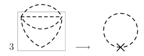
Figure 1: The appearance of vertex type subdivergences in the first double integral of (29) as illustrated at leading $\lambda$ order in the expansion of the denominator of the integrand. The factor of three indicates the possible ways in which two lines of the setting-sun diagram form the bubble which corrects the vertex at 2-loop level. The cross denotes the associated lowest order counterterm.

The double integral $\tilde{J}_{\textnormal{div}}(M^{2})$ has also a vertex type subdivergence as illustrated in Fig. 1 at leading order of the expansion in $\lambda.$ This is canceled, as it should, by the last integral of (30). One can see this analytically by separating in the difference of the two terms of the square bracket of (30) a contribution proportional to $T_{a}^{(I)}T_{\pi}^{F}$ which on its turn cancels against the contribution of the last tadpole integral in (30).

With all subdivergences and $v^{2}$-dependent divergences of (30) canceled, $\delta\Delta\Gamma^{\alpha,0}(\hat{\alpha})/\delta\hat{\alpha}$ is determined by the overall divergence of $\tilde{J}(M^{2})$ and that of the last tadpole integral. Its expression reads:

$$\frac{\delta\Delta\Gamma^{\alpha,0}(\hat{\alpha})}{\delta\hat{\alpha}} = iT_{d}^{(2)}+i(4M^{2}-M_{0}^{2})T_{d}^{(0)}-iT_{a}^{(2)}\left(1+\frac{\lambda}{6}T_{d}^{(0)}+\frac{\lambda}{48\pi^{2}}\right)$$ (31)

$$+iT_{a}^{(I)}\left[\lambda\left(M^{2}-\frac{1}{2}M_{0}^{2}\right)+\frac{\lambda^{2}}{6}T_{d}^{(0)}\left(M^{2}-M_{0}^{2}\right)+\frac{\lambda^{2}}{12}T_{d}^{(2)}+\frac{\lambda^{2}}{12}\frac{3M^{2}-M_{0}^{2}}{16\pi^{2}}\right].$$

Since the above expression depends only on $\hat{\alpha}$ it will have no “back-reaction” neither on the propagator equations nor on the derivative of the effective potential with respect to the background. The appearance of terms proportional to $1/(16\pi^{2})$ reflects some allowed arbitrariness of the subtraction procedure.

We do not present here the renormalisation of the partial NLO corrections which would occur in the $\alpha-\sigma$ sector should one use the effective action functional (7). All counterterms necessary for the renormalisation of these pieces are of ${\cal O}(1/N)$, not contributing to the renormalised effective action at NLO in the $1/N$ expansion.

In conclusion, only divergences proportional to zeroth or first powers of $M^{2}$ remained which upon integration over $\hat{\alpha}$ determine the $\hat{\alpha}$-dependent counterterm functional $\Delta\Gamma^{\alpha,0}(\hat{\alpha}).$ The counterterms induced by the renormalization of the NLO pion propagator and of $\delta\Gamma/\delta v$ played an essential role in the cancellation of subdivergences and of $v^{2}$-dependent divergences present in the expression of $\delta\Gamma/\delta\hat{\alpha}.$ No limitations whatsoever showed up on the value of $M^{2}$ and/or $v^{2},$ in contrast to the findings in andersen04 ; andersen08 . We shall return to the discussion of this difference after reducing the effective action to the effective potential depending only on the background fields in Appendix B. The functional corresponding to the NLO $1/N$-expansion of the classical vertex approximation (BVA) is renormalized without any constraint. Our result shows that this can be achieved also without introducing unconventional counterterms jakovac08 .

V The explicit form of the counterterm functional

In this section we collect into a unique expression $\Delta\Gamma$ all individual pieces determined in Eqs. (10), (14), (23), (25), (31), and express it in a conventional form, in which one associates them with the renormalization of different couplings appearing in the terms of $\Gamma[\hat{\alpha},v,G_{\pi},{\cal G}]$ (Eq. (8)). The counterterm functional reads:

$$\Delta\Gamma[\hat{\alpha},v,G_{\pi},{\cal G}] = \frac{1}{2}\left(\delta m^{2}-i\delta g\hat{\alpha}\right)v^{2}+i\delta\kappa_{1}\hat{\alpha}+\delta\kappa_{2}\hat{\alpha}^{2}$$ (32)

$$+ \frac{1}{2}(\delta m^{2}-i\delta g\hat{\alpha})\int_{k}G_{\pi}(k)+\frac{1}{2}\delta\kappa_{0}\int_{k}G_{\alpha\alpha}(k),$$

where the counter-couplings are given by the following expressions:

$$\delta m^{2} = -\frac{\lambda}{3}\left[T_{a}^{(2)}-\frac{\lambda}{2}\left(m^{2}-M_{0}^{2}\right)T_{a}^{(I)}\right],\qquad\delta g=\frac{\lambda^{2}}{6}T_{a}^{(I)},$$

$$\qquad\delta\kappa_{2} = \frac{N+8}{4}T_{d}^{(0)}+\frac{\lambda}{2}T_{a}^{(I)}\left(1+\frac{\lambda}{6}T_{d}^{(0)}+\frac{\lambda}{64\pi^{2}}\right),\qquad\delta\kappa_{0}=\frac{\lambda}{6}T_{d}^{(0)},$$

$$\delta\kappa_{1} = \frac{N}{2}\left[T_{d}^{(2)}+(m^{2}-M_{0}^{2})T_{d}^{(0)}\right]+T_{d}^{(2)}+(4m^{2}-M_{0}^{2})T_{d}^{(0)}-T_{a}^{(2)}\left(1+\frac{\lambda}{6}T_{d}^{(0)}+\frac{\lambda}{48\pi^{2}}\right)$$ (33)

$$+\lambda T_{a}^{(I)}\left[m^{2}-\frac{1}{2}M_{0}^{2}+\frac{\lambda}{12}\left(2T_{d}^{(0)}(m^{2}-M_{0}^{2})+T_{d}^{(2)}+\frac{1}{16\pi^{2}}(3m^{2}-M_{0}^{2})\right)\right].$$

It is interesting to note that the term proportional to $\delta\kappa_{1}$ in (32) has no correspondent in (8). Moreover, the terms proportional to $\delta\kappa_{0}$ and $\delta\kappa_{2}$ correspond in (8) to terms not proportional to any coupling of the original theory. Rather they renormalize numerical coefficients related to the way the auxiliary field $\alpha$ is introduced by the parametrization of the Hubbard-Stratonovich transformation (cf. (1)). They correspond to different possibilities of defining the two-point function of the auxiliary field. They are calculated to different orders in $1/N$ since the corresponding terms contribute at different levels of the expansion. After scaling back the fluctuating part of the field $\hat{\alpha}$ to $\alpha$ the two counter couplings do agree to leading order in $1/N$. This feature is reminiscent of the renormalisation of the operators corresponding to different definitions of the n-point functions in 2PI-approximations. The terms with $\delta g$ can be regarded as renormalizing the coupling $g=\sqrt{\lambda/(3N)}$ through which the auxiliary field couples to fields of the $O(N)$ multiplet. One interprets the renormalisation of all these operators not occuring in the original model as renormalisations of the two variants of the 2-point functions of the composite field $\phi^{2}$ and of the $\phi^{2}\sigma\sigma$ vertex (see ch. 30 of zinn-justin02 ).

It is notable that $\delta\kappa_{2}$ determines the renormalization of the coupling $\lambda$ following the formula

$$\frac{6}{\lambda_{B}}=\frac{6}{\lambda}+\frac{4}{N}\delta\kappa_{2}=\frac{6}{\lambda}+\frac{N+8}{N}T_{d}^{(0)}+2\frac{\lambda}{N}T_{a}^{(I)}\left(1+\frac{\lambda}{6}T_{d}^{(0)}+\frac{\lambda}{64\pi^{2}}\right).$$ (34)

This can be seen by looking at the terms proportional to $\hat{\alpha}^{2}$ in the classical part of the functional. This relation is only intermediary, since it will change in the course of the elimination of $\hat{\alpha}$. The part of the counterterm $\delta\kappa_{2}$ proportional solely to $T_{d}^{(0)}$ appears already in the literature and follows the one-loop $\beta$-function of the model kleinert . The entire NLO part of $\delta\kappa_{2}$ proportional to $T_{a}^{(I)}$ is missing in the analysis of andersen04 ; andersen08 (see e.g. Eq. (23) of andersen08 for the expression of their counterterm $b_{1}$).

Introducing the following notations

$$\delta\kappa_{2}=N\delta\kappa_{2}^{(0)}+\delta\kappa_{2}^{(1)},\qquad\lambda_{B}=\lambda+\delta\lambda_{\alpha},\qquad\delta\lambda_{\alpha}=\delta\lambda_{\alpha}^{(0)}+\frac{1}{N}\delta\lambda_{\alpha}^{(1)},$$ (35)

one readily obtains

$$\delta\lambda_{\alpha}^{(0)}=-\frac{\lambda^{2}}{6}\frac{T_{d}^{(0)}}{1+\lambda T_{d}^{(0)}/6},\qquad\lambda_{B}^{(0)}=\lambda+\delta\lambda_{\alpha}^{(0)}=\frac{\lambda}{1+\lambda T_{d}^{(0)}/6},\qquad\delta\lambda_{\alpha}^{(1)}=-\frac{2}{3}\big{(}\lambda_{B}^{(0)}\big{)}^{2}\delta\kappa_{2}^{(1)}.$$ (36)

Comparing with Eq. (25) of fejos08 one observes that $\delta\lambda_{\alpha}^{(0)}$ is the counter-coupling of the $O(N)$ model formulated with its original variables and considered at LO in the large-$N$ expansion. Likewise $\lambda_{B}^{(0)}$ is the bare coupling of the model in the large-$N$ limit. We shall see in the next section, where the auxiliary field will be eliminated, that at NLO in the large-$N$ expansion the bare coupling of the $O(N)$ model differs from $\lambda_{B},$ it turns out to be a combination of $\lambda_{B}$ and $\delta g$ (see (46) and (47)).

With the counterterm functional $\Delta\Gamma$ explicitly determined by (32), one can give now in a compact form the functional introduced in (8):

$$\Gamma_{\textnormal{NLO}}[\hat{\alpha},v,G_{\pi},{\cal G}] = \frac{N}{2}(m_{B}^{2}-i\hat{c}\hat{\alpha})v^{2}+i\delta\kappa_{1}\hat{\alpha}+\frac{3N}{2\lambda_{B}}\hat{\alpha}^{2}-\frac{i}{2}\int_{k}[\textnormal{Tr}\ln{\cal G}^{-1}(k)+(N-1)\ln G_{\pi}^{-1}(k)]$$ (37)

$$-\frac{1}{2}\int_{k}\big{[}k^{2}-m_{B}^{2}+i\hat{c}\hat{\alpha}\big{]}\big{[}(N-1)G_{\pi}(k)+G_{\sigma\sigma}^{(0)}(k)\big{]}-iv\sqrt{\frac{\lambda}{3}}\int_{k}G_{\alpha\sigma}^{(0)}(k)$$

$$+\frac{c}{2}\int_{k}G_{\alpha\alpha}^{(0)}(k)-\frac{\lambda}{12}\int_{k}G_{\alpha\alpha}^{(0)}(k)\Pi(k),$$

where $\lambda_{B}$ is defined in (34) and we introduced the following notations:

$$m_{B}^{2}=m^{2}+\frac{1}{N}\delta m^{2},\qquad\hat{c}=1+\frac{1}{N}\delta g,\qquad c=1+\delta\kappa_{0},\qquad\Pi(k)=-i\int_{p}G_{\pi}(p)G_{\pi}(k+p).$$ (38)

VI Elimination of the auxiliary field

In this section the ${\cal O}(N^{0})$ accurate renormalized functional will be established for the original formulation of the $O(N)$ model by eliminating the auxiliary field $\hat{\alpha}$ and the propagator components related to it (i.e. $G_{\alpha\sigma}$ and $G_{\alpha\alpha}$). In order to achieve this one substitutes into (37) the expressions of $\hat{\alpha},G_{\alpha\sigma}^{(0)},$ and $G_{\alpha\alpha}^{(0)}$ as found from their respective equations.

VI.1 Determination of $\Gamma_{\textnormal{NLO}}[v,G_{\pi},G_{\sigma}]$

For rewriting the terms depending on $G_{\alpha\alpha}^{(0)}$ and $G_{\alpha\sigma}^{(0)}$ one exploits their representations which allow the expression of the result fully in terms of $\Pi(k)$ and $G_{\sigma\sigma}^{(0)}.$ The latter will be replaced with $G_{\sigma},$ the exact sigma propagator of the $O(N)$ model. In this way one finds

$$-\frac{i}{2}\int_{k}\textnormal{Tr}\ln{\cal G}^{-1}(k) = -\frac{i}{2}\int_{k}\ln\textnormal{det}{\cal G}^{-1}(k)=-\frac{i}{2}\int_{k}\ln\left[\left(1-\frac{\lambda}{6}I_{\pi}^{F}(k)\right)iG_{\sigma}^{-1}(k)\right]$$ (39)

$$= -\frac{i}{2}\int_{k}\ln G_{\sigma}^{-1}(k)-\frac{i}{2}\int_{k}\ln\left(1-\frac{\lambda}{6c}\Pi(k)\right)-\frac{i}{2}\int_{k}\ln(ic)+{\cal O}\left(\frac{1}{N}\right).$$

In going from the first to the second line above we used that to ${\cal O}(1/N)$ accuracy

$$-i\int_{p}G_{\pi}(p)G_{\pi}(k+p)\Big{|}_{\textnormal{div}}=-i\int_{p}D_{\pi}(p)D_{\pi}(k+p)\Big{|}_{\textnormal{div}}=T_{d}^{(0)},$$ (40)

and therefore one has

$$1-\frac{\lambda}{6}I_{\pi}^{F}(k)=c-\frac{\lambda}{6}I_{\pi}(k)=c-\frac{\lambda}{6}\Pi(k)+{\cal O}\left(\frac{1}{N}\right),$$ (41)

where the neglected ${\cal O}(1/N)$ contribution is finite.

Using (19) for $G_{\alpha\alpha}^{(0)}$ one writes the following chain of expressions for the last term of (37):

$$-\frac{\lambda}{12}\int_{k}G_{\alpha\alpha}^{(0)}(k)\Pi(k) = -\frac{c}{2}\int_{k}G_{\alpha\alpha}^{(0)}(k)+\frac{1}{2}\int_{k}G_{\alpha\alpha}^{(0)}(k)\left(c-\frac{\lambda}{6}\Pi(k)\right)$$ (42)

$$= -\frac{c}{2}\int_{k}G_{\alpha\alpha}^{(0)}(k)-\frac{\lambda}{6c}v^{2}\int_{k}\frac{G_{\sigma}(k)}{1-\frac{\lambda}{6c}\Pi(k)}-\frac{i}{2}\int_{k}1+{\cal O}\left(\frac{1}{N}\right).$$

In writing the second line above one again uses (41). The first term on the r.h.s. above is canceled against the last but one term of (37). Finally, for the last term in the second line of (37) one uses (41) to write:

$$-iv\sqrt{\frac{\lambda}{3}}\int_{k}G_{\alpha\sigma}^{(0)}(k)=\frac{\lambda}{3c}v^{2}\int_{k}\frac{G_{\sigma}(k)}{1-\frac{\lambda}{6c}\Pi(k)}+{\cal O}\left(\frac{1}{N}\right).$$ (43)

As a short digression from our current task we mention that one could proceed by further eliminating also the pion and sigma propagators using their respective NLO and LO equations. Then one obtains the renormalized version of the effective potential as function of $\hat{\alpha}$ and $v$ studied in andersen04 ; andersen08 . A sketch of this derivation is presented in Appendix B together with a check of the renormalization of the saddle point equation coming from this potential.

Now, we proceed instead with the elimination of $\hat{\alpha}$ from (37) keeping the variables of the original theory, i.e. $v,G_{\pi},$ and $G_{\sigma}$. Actually, the simplest way is to complete to full square the functional depending quadratically on $\hat{\alpha}$ and then to use the saddle point equation $\delta\Gamma/\delta\hat{\alpha}=0.$ Replacing $G_{\sigma\sigma}^{(0)}$ by the exact propagator $G_{\sigma}$ of the $O(N)$ model one obtains from the $\hat{\alpha}$-dependent part

$$\frac{\lambda_{B}}{24N}\left[N\hat{c}v^{2}+\hat{c}\int_{k}\big{[}(N-1)G_{\pi}(k)+G_{\sigma}(k)\big{]}-2\delta\kappa_{1}\right]^{2}.$$ (44)

Putting together all above pieces one also uses that in view of (36) $\lambda/c=\lambda_{B}^{(0)}$ and obtains

$$\Gamma[v,G_{\pi},G_{\sigma}] = \frac{N}{2}\left(m_{B}^{2}-\frac{\lambda_{B}\hat{c}\delta\kappa_{1}}{3N}\right)v^{2}+N\frac{\lambda_{B}\hat{c}^{2}}{24}v^{4}-\frac{i}{2}\int_{k}\big{[}(N-1)\ln G_{\pi}^{-1}(k)+\ln G_{\sigma}^{-1}(k)\big{]}$$ (45)

$$-\frac{1}{2}\int_{k}\left[k^{2}-m_{B}^{2}+\frac{\lambda_{B}\hat{c}\delta\kappa_{1}}{3N}-\frac{\lambda_{B}\hat{c}^{2}}{6}v^{2}\right]\big{[}(N-1)G_{\pi}(k)+G_{\sigma}(k)\big{]}$$

$$+\frac{\lambda_{B}^{(0)}}{6}v^{2}\int_{k}\frac{G_{\sigma}(k)}{1-\lambda_{B}^{(0)}\Pi(k)/6}-\frac{i}{2}\int_{k}\ln\bigg{(}1-\frac{\lambda_{B}^{(0)}}{6}\Pi(k)\bigg{)}$$

$$+\frac{\lambda_{B}\hat{c}^{2}}{24}(N-2)\left(\int_{k}G_{\pi}(k)\right)^{2}+\frac{\lambda_{B}\hat{c}^{2}}{12}\int_{k}G_{\pi}(k)\int_{p}G_{\sigma}(p),$$

where we omitted terms of order ${\cal O}(1/N)$ and a divergent constant $\sim\delta\kappa_{1}^{2}$ coming from (44) as well as the irrelevant divergent last but one terms of (39) and (42).

The bare couplings appearing in (45) have to be given with an accuracy corresponding to that of the functional (8), therefore one writes the counterterms as a sum of the LO and NLO contributions:

$$\lambda_{B}\hat{c}^{2}=\lambda+\delta\lambda,\qquad \delta\lambda=\delta\lambda^{(0)}+\frac{1}{N}\delta\lambda^{(1)},$$

$$m_{B}^{2}-\frac{\lambda_{B}\hat{c}\delta\kappa_{1}}{3N}=m^{2}+\delta m^{2},\qquad \delta m^{2}=\delta{m^{2}}^{(0)}+\frac{1}{N}\delta{m^{2}}^{(1)}.$$ (46)

With help of (34), (35), (36), (38) and the separation $\delta\kappa_{1}=N\delta\kappa_{1}^{(0)}+\delta\kappa_{1}^{(1)},$ the counter-couplings above can be given in terms of the counter-couplings of the model in the auxiliary field formalism as

$$\delta\lambda^{(0)}=\delta\lambda_{\alpha}^{(0)},\qquad \delta\lambda^{(1)}=\delta\lambda_{\alpha}^{(1)}+2\lambda_{B}^{(0)}\delta g,$$

$$\delta{m^{2}}^{(0)}=-\frac{1}{3}\lambda_{B}^{(0)}\delta\kappa_{1}^{(0)},\qquad \delta{m^{2}}^{(1)}=\delta m^{2}-\frac{1}{3}\left[\delta\lambda_{\alpha}^{(1)}\delta\kappa_{1}^{(0)}+\lambda_{B}^{(0)}\left(\delta\kappa_{1}^{(1)}+\delta\kappa_{1}^{(0)}\delta g\right)\right].$$ (47)

Using (46) in (45) one obtains at NLO in the $1/N$ expansion the renormalized functional of the original $O(N)$ model, that is without the auxiliary field, in the following form:

$$\Gamma_{\textnormal{NLO}}[v,G_{\pi},G_{\sigma}] = -\frac{i}{2}\int_{k}\left[(N-1)\left(\ln G_{\pi}^{-1}(k)+\mathscr{D}^{-1}_{\pi}(k)G_{\pi}(k)\right)+\ln G_{\sigma}^{-1}(k)+\mathscr{D}^{-1}_{\sigma}(k)G_{\sigma}(k)\right]$$ (48)

$$+ \frac{N}{2}m^{2}v^{2}+N\frac{\lambda}{24}v^{4}+N\frac{\lambda}{24}\left(\int_{k}G_{\pi}(k)\right)^{2}+\frac{\lambda}{12}\int_{k}G_{\pi}(k)\int_{p}G_{\sigma}(p)$$

$$- \frac{\lambda_{B}^{(0)}}{6}v^{2}\int_{k}G_{\sigma}(k)+\frac{\lambda_{B}^{(0)}}{6}v^{2}\int_{k}\frac{G_{\sigma}(k)}{1-\lambda_{B}^{(0)}\Pi(k)/6}$$

$$- \frac{\lambda_{B}^{(0)}}{12}\left(\int_{k}G_{\pi}(k)\right)^{2}-\frac{i}{2}\int_{k}\ln\bigg{(}1-\frac{\lambda_{B}^{(0)}}{6}\Pi(k)\bigg{)}$$

$$+ \frac{N}{2}\delta m^{2}v^{2}+N\frac{\delta\lambda}{24}v^{4}+\frac{\delta m^{2}}{2}\int_{k}\big{[}(N-1)G_{\pi}(k)+G_{\sigma}(k)\big{]}$$

$$+ \frac{\delta\lambda}{12}\left[v^{2}\int_{k}\big{[}(N-1)G_{\pi}(k)+3G_{\sigma}(k)\big{]}+\frac{N}{2}\left[\int_{k}G_{\pi}(k)\right]^{2}+\int_{k}G_{\pi}(k)\int_{p}G_{\sigma}(p)\right],\ \ \ \$$

where we introduced the usual tree-level propagators for the sigma and pion fields as

$$i\mathscr{D}^{-1}_{\sigma}(k)=k^{2}-m^{2}-\frac{\lambda}{2}v^{2},\qquad i\mathscr{D}^{-1}_{\pi}(k)=k^{2}-m^{2}-\frac{\lambda}{6}v^{2}.$$ (49)

If one forgets about the counterterms, the expression in (48) coincides with the 2PI effective potential obtained in dominici93 . The terms above can be combined in a way which makes explicit that in the large-$N$ expansion there are only two bare couplings, namely $m^{2}+\delta m^{2}$ and $\lambda+\delta\lambda$. Would one attempt a selfconsistent solution of the equations arising from the variation of $\Gamma_{\textnormal{NLO}}$ this would not be true (see the concluding part of this subsection). We emphasize also that since the above functional is ${\cal O}(N^{0})$ accurate, in terms involving the sigma propagator $G_{\sigma}$ one does not need the NLO part of the counterterms, i.e. $\delta m^{2^{(1)}}$ and $\delta\lambda^{(1)}.$ When differentiating with respect to $G_{\pi}$ one should remember that also $\Pi(k)$ is a functional of $G_{\pi}!$

The interpretation of the terms in (48), which makes explicit the infinite series of diagrams summed up in the present treatment is as follows. The first two and the last two lines represent the 2PI effective potential of the $O(N)$ model at Hartree level of the truncation and at NLO in its large-$N$ expansion. The remaining four terms represent the NLO contribution of the 2PI vacuum diagrams beyond Hartree level. The $v^{2}$-dependent part of these terms can be rewritten as

$$\frac{\lambda+\delta\lambda^{(0)}}{6}v^{2}\int_{k}G_{\sigma}(k)\frac{\big{(}\lambda+\delta\lambda^{(0)}\big{)}\Pi(k)/6}{1-\big{(}\lambda+\delta\lambda^{(0)}\big{)}\Pi(k)/6}=\frac{\lambda+\delta\lambda^{(0)}}{6}v^{2}\int_{k}G_{\sigma}(k)\sum_{n=1}^{\infty}\left(\frac{\lambda+\delta\lambda^{(0)}}{6}\Pi(k)\right)^{n}.$$ (50)

The $v^{2}$-independent part can also be written as a sum:

$$-\frac{i}{2}\left[\frac{\lambda+\delta\lambda^{(0)}}{6}\int_{k}\Pi(k)+\int_{k}\ln\bigg{(}1-\frac{\lambda+\delta\lambda^{(0)}}{6}\Pi(k)\bigg{)}\right]=\frac{i}{2}\int_{k}\sum_{n=2}^{\infty}\frac{1}{n}\left(\frac{\lambda+\delta\lambda^{(0)}}{6}\Pi(k)\right)^{n}.$$ (51)

It is easy to show that not considering counterterms, these terms correspond to the two sets of diagrams given in Fig. 2. Counterterm diagrams corresponding to the $n=2$ term of the sum in (50) are displayed in Fig. 3. Similar diagrams with different number of pion bubbles can be drawn for the other terms appearing in the sums in (50) and (51). A direct way to obtain (48) consists of summing up all these diagrams with the associated combinatorial factors determined by the Feynman rules.

Figure 2: The two sets of vacuum diagrams which contribute beyond Hartree level and at NLO to the 2PI functional. Solid (dashed) line represents sigma (pion) propagator, while wiggly line represents the background $v.$ The dots indicate any number of pion bubbles.

Figure 3: Diagrams corresponding to the $n=2$ term in the sum on the r.h.s. of (50). The cross represents the counter-coupling $\delta\lambda^{(0)}.$

An interesting question is how the counterterms of the last two lines of (48) are related to the set of counterterms introduced in berges05 . That structure was fixed by the possible $O(N)$ invariants of the model. Comparing the expressions presented in Eq. (6) of fejos08 with those of the last two lines of (48) one obtains the following unique relation for all of them:

$$\delta\lambda_{4}=\delta\lambda_{2}^{A}=\delta\lambda_{0}^{A}=\delta\lambda_{2}^{B}=\delta\lambda_{0}^{B}=\delta\lambda,\qquad\delta m^{2}_{2}=\delta m^{2}_{0}=\delta m^{2}.$$ (52)

This result is actually expected on general grounds, since in the strict $1/N$ expansion used in our approach different definitions of the two- and four-point functions coincide. The above coincidence represents rather a check of the correctness of our NLO renormalization.

VI.2 Renormalizability checks on $\Gamma_{\textnormal{NLO}}[v,G_{\pi},G_{\sigma}]$

The significance of (48) is that it displays all counterterms which guarantee the renormalizability of the resummation of the perturbative series, a resummation induced by the large-$N$ expansion. The finiteness of the equation of state and the self-energies obtained from its respective variations is ensured automatically, since this feature is “inherited” from the finiteness of the same quantities achieved in the formulation with the auxiliary field. Still, it is an instructive exercise to check this feature directly. Exploiting the structure of our previous analysis done in the auxiliary formulation of the model we shall show the finiteness of the equations directly obtained from (48).

The inverse pion propagator at NLO in the $1/N$ expansion is given then by

$$iG_{\pi}^{-1}(k)=k^{2}-M^{2}-\frac{\lambda}{3N}\Sigma_{\pi}^{F}(k),$$ (53)

where the nonlocal and local parts of the self-energy are:

$$\Sigma_{\pi}^{F}(k) = i\int_{p}\left[-\frac{i}{1-\lambda\Pi_{F}(p)/6}-\frac{\lambda v^{2}}{3}\frac{G_{\sigma}(p)}{\left(1-\lambda\Pi_{F}(p)/6\right)^{2}}\right]G_{\pi}(k+p)-\tilde{T}_{\textnormal{div}}(M^{2}),$$

$$M^{2} = m_{B}^{2}+\frac{\lambda_{B}}{6}\left(v^{2}+\int_{k}G_{\pi}(k)\right)+\frac{\lambda_{B}}{6N}\int_{k}\Big{(}G_{\sigma}(k)-G_{\pi}(k)\Big{)}+\frac{\lambda}{3N}\tilde{T}_{\textnormal{div}}(M^{2}).$$ (54)

For the nonlocal part we used that $6/\lambda_{B}^{(0)}-\Pi=6/\lambda-\Pi_{F}/6$ and $\tilde{T}_{\textnormal{div}}$ is given in (21).

Since the local part has LO and NLO contributions one writes $M^{2}={M^{2}}^{(0)}+{M^{2}}^{(1)}/N$ and expands the pion propagator to ${\cal O}(1/N)$. With help of the integrals defined in (29) one obtains

$${M^{2}}^{(0)}=m^{2}+\delta{m^{2}}^{(0)}+\frac{\lambda_{B}^{(0)}}{6}\left(v^{2}+\int_{k}D_{\pi}(k)\right),$$

$$3i\frac{{M^{2}}^{(1)}}{\lambda_{B}^{(0)}}\left(1-\frac{\lambda_{B}^{(0)}}{6}I_{\pi}(0)\right)=\frac{3i}{\lambda_{B}^{(0)}}\left[\delta{m^{2}}^{(1)}+\frac{\lambda}{3}\tilde{T}_{\textnormal{div}}\big{(}{M^{2}}^{(0)}\big{)}\right]+\frac{i}{2}\int_{k}\Big{(}G_{\sigma}(k)-D_{\pi}(k)\Big{)}$$

$$\qquad\ +\frac{\lambda}{6}\left[\tilde{J}({M^{2}}^{(0)})-\tilde{T}_{\textnormal{div}}({M^{2}}^{(0)})\int_{k}D_{\pi}^{2}(k)\right]-i\frac{\lambda^{2}}{18}v^{2}J({M^{2}}^{(0)})+\frac{i\delta\lambda^{(1)}}{2\lambda_{B}^{(0)}}\left(v^{2}+\int_{k}D_{\pi}(k)\right),$$ (55)

where in comparison to its definition given in (5) $D_{\pi}$ depends now on ${M^{2}}^{(0)}.$ We used also that to leading order $\Pi(p)=I_{\pi}(p).$

The equation for ${M^{2}}^{(0)}$ in (55) is the usual gap equation at Hartree level of truncation of the effective action. This was analyzed in fejos08 and the counterterms which can be determine from this are $\delta\lambda^{(0)}$ and $\delta{m^{2}}^{(0)}$ given in (47).

Observing that the left hand side of the equation for ${M^{2}}^{(1)}$ in (55) is finite one obtains the following relation between counterterms and divergences:

$$-\frac{3i}{\lambda_{B}^{(0)}}\left[\delta{m^{2}}^{(1)}+\frac{\lambda}{3}\tilde{T}_{\textnormal{div}}\big{(}{M^{2}}^{(0)}\big{)}\right] = \frac{\lambda}{6}\left[\tilde{J}_{\textnormal{div}}({M^{2}}^{(0)})-\tilde{T}_{\textnormal{div}}({M^{2}}^{(0)})\int_{k}D_{\pi}^{2}(k)\right]-i\frac{\lambda^{2}}{18}v^{2}J_{\textnormal{div}}({M^{2}}^{(0)})$$ (56)

$$+\frac{i\delta\lambda^{(1)}}{2\lambda_{B}^{(0)}}\left(v^{2}+\int_{k}D_{\pi}(k)\right)+\frac{i}{2}\int_{k}\Big{(}G_{\sigma}(k)-D_{\pi}(k)\Big{)}\bigg{|}_{\textnormal{div}}.$$

Using the divergence analysis of Appendix A one has all divergences and integrals expressed in terms of ${M^{2}}^{(0)}$ for which one can substitute its finite gap equation ${M^{2}}^{(0)}=m^{2}+\lambda/6(v^{2}+T_{\pi}^{F}).$ Requiring the vanishing of the coefficient of $v^{2}+T_{\pi}^{F}$ determines $\delta\lambda^{(1)},$ while the remaining overall divergence determines $\delta{m^{2}}^{(1)}.$ Both are in accordance with (47).

The equation for the inverse sigma propagator obtained from (48) is

$$iG_{\sigma}^{-1}(k)=k^{2}-{M^{2}}^{(0)}-\frac{\lambda_{B}^{(0)}}{3}v^{2}\frac{1}{1-\lambda_{B}^{(0)}I_{\pi}(k)/6},$$ (57)

which is finite, since ${M^{2}}^{(0)}$ is finite and $6/\lambda_{B}^{(0)}-I_{\pi}=6/\lambda-I_{\pi}^{F}/6.$

Using the relation between the LO pion and sigma propagators one can show that the derivative of (48) with respect to $v$ reads as

$$\frac{\delta\Gamma_{\textnormal{NLO}}}{\delta v}[v,G_{\pi},G_{\sigma}]=-NviG_{\pi}^{-1}(k=0),$$ (58)

which is also finite, since we showed that $G_{\pi}^{-1}(k)$ is finite. It also displays the validity of Goldstone’s theorem.

We close this part by mentioning that the LO sigma propagator equation, the NLO pion propagator equation and the equation of state derived from (48) can be obtained also with the Dyson-Schwinger formalism of Section 2. Concerning these equations, the large-$N$ expansion closes the hierarchy of DS equations at the level of complete LO renormalized $\Gamma_{\pi\pi\sigma}$ and $\Gamma_{\pi\pi\pi\pi}$ vertex functions, which include also one-loop pion corrections. Some details can be found in patkos06 for $G_{\sigma}$ and $\Gamma_{\pi\pi\sigma}$ (see also korpa for the relation between the truncation of the Dyson-Schwinger equations and the $1/N$ expansion). This means that our investigation implies also the renormalizability of the Dyson-Schwinger equations at NLO in the large-$N$ expansion.

VII Conclusions

We studied the renormalizability of the $O(N)$ model at next-to-leading order in the large-$N$ expansion, at zero temperature. We constructed the ${\cal O}(N^{0})$ counterterm functional of the model in auxiliary field formalism by studying the renormalization of the derivatives of a generalized effective action functional with respect to its variables. Expanding the propagator equation of the pion to ${\cal O}(1/N)$ in the large-$N$ expansion we showed that the renormalization can be achieved for arbitrary values of the background and auxiliary field, in a way that respects the internal symmetry of the model (e.g. Goldstone’s theorem). This can be expected on theoretical grounds, since divergences are determined only by the asymptotic behavior of the propagators and because any consistent resummation of the perturbation theory should resum also the counterterm diagrams associated to the perturbative series. Although, one can anticipate the consistency of the auxiliary field technique and of the large-$N$ expansion in dealing with perturbative series, the difficulty we face when trying to infer the renormalizability of the model in a given approximation from the fact that the model is perturbatively renormalizable is that one cannot easily keep track of what partial series of counterterm diagrams is actually resummed at a given order of the large-$N$ expansion. In consequence, the actual analytic check of the renormalization of a given approximation is unavoidable.

The elimination of the auxiliary field and the related propagators, while keeping the dynamical sigma and pion propagators, makes transparent the classes of diagrams containing also counterterms which are resummed in the original $O(N)$ theory at NLO of the large-$N$ expansion. The explicit form of the counterterms is given here for the first time for the theory using auxiliary field and also for the original formulation. In the original theory the action functional contains only two counterterms, a coupling and a mass counterterm, both having LO and NLO parts. The propagator equations and the equation of state derived from that coincides with the 1PI Schwinger-Dyson equations closed at the complete LO $\Gamma_{\pi\pi\sigma}$ and $\Gamma_{\pi\pi\pi\pi}$ vertex functions, which includes one-loop pion corrections.

The two examples we worked out (e.g. $\Gamma_{\textnormal{NLO}}[v,G_{\pi},G_{\sigma}]$ and $\Gamma_{\textnormal{NLO}}[\hat{\alpha},v]$) demonstrate that the renormalizability of the broadest action functional $\Gamma[\hat{\alpha},v,G_{\pi},{\cal G}]$ implies the renormalizability of the functionals arising after the elimination of some subset of the variables. This result obtained at $T=0$ makes us confident that the renormalization goes through for nonzero temperature as well and that the counterterm functional determined here will prove helpful for phenomenological studies in the $O(N)$ model. A study of the renormalization scale invariance at NLO in different formulations would be helpful for such applications. The method developed here can be used also to models with more complicated global symmetries.

Appendix A Detailed analysis of the divergences

Notations

Following the spirit of Ref. patkos08 we will expand the propagators around appropriately chosen infrared safe auxiliary propagators. Since at NLO the asymptotics is determined basically by integrals of the LO propagator $D_{\pi}(p)$ and of the propagator $\tilde{G}(p)$ given in (16) which incorporates the effect of the resummation of the chain of pion bubbles, one needs two auxiliary propagators. The first one is

$$G_{0}(p)=\frac{i}{p^{2}-M_{0}^{2}},$$ (59)

where $M_{0}$ is an arbitrary mass scale. With this propagator one defines the quadratically divergent integral

$$T_{d}^{(2)}=\int_{p}G_{0}(p),$$ (60)

and the following one-loop bubble integral

$$I_{0}(p)=-i\int_{k}G_{0}(k)G_{0}(k+p)=T_{d}^{(0)}+I_{0}^{F}(p).$$ (61)

The logarithmically divergent part of the integral above is defined as

$$T_{d}^{(0)}=-i\int_{k}G_{0}^{2}(k).$$ (62)

The finite part behaves asymptotically as $I_{0}^{F}(p)\sim\ln\frac{p^{2}}{M_{0}^{2}}-2-i\pi+{\cal O}\left(p^{-2}\ln p\right),$ and defines together with $G_{0}(p)$ the second auxiliary propagator:

$$G_{a}(p)=\frac{i}{(p^{2}-M_{0}^{2})(1-\lambda I_{0}^{F}(p)/6)}.$$ (63)

The integrals involving only combinations of $G_{0}(p),$ $G_{a}(p)$ and $I_{0}^{F}(p)$ will be fully included in the counterterms. With help of the propagator $G_{0}(p)$ one can separate the quadratic and logarithmic divergence of the tadpole integral defined with the tree-level propagator given in (5). At zero temperature one has:

$$\int_{k}D_{\pi}(k)=T_{d}^{(2)}+\left(M^{2}-M_{0}^{2}\right)T_{d}^{(0)}+T_{\pi}^{F},\qquad T_{\pi}^{F}=\frac{1}{16\pi^{2}}\left(M^{2}\ln\frac{M^{2}}{M_{0}^{2}}-M^{2}+M_{0}^{2}\right).$$ (64)

Absence of wave function renormalization in the NLO pion propagator

The only term which on dimensional grounds could produce a momentum-dependent divergence in the expression of the NLO pion propagator (18) is the first one on the r.h.s. of (19). It gives the integral

$$\int_{p}\frac{D_{\pi}(p+k)}{1-\lambda I_{\pi}^{F}(p)/6}.$$ (65)

To study this integral one uses the following expansion

$$-iD_{\pi}(p+k)=\frac{1}{(p+k)^{2}-M^{2}}=\frac{1}{p^{2}-M^{2}}+\frac{1}{p^{2}-M^{2}}\sum_{n=1}^{\infty}\left(-\frac{k^{2}+2p\cdot k}{p^{2}-M^{2}}\right)^{n}.$$ (66)

In order to prove that there is no infinite wave function renormalization it is enough to look at the appearance of $k^{2}$ in the numerator, that is at terms $n=1,2$ in the sum. Keeping only terms up to and including ${\cal O}(1/p^{4}),$ but throwing away those which vanish upon symmetrical integration (note that $I_{\pi}^{F}(p)$ depends on $p^{2}$) amounts to the following replacement at the level of the integrand in (65) :

$$\frac{1}{(p+k)^{2}-M^{2}}\longrightarrow\frac{1}{p^{2}-M^{2}}+\frac{4(p\cdot k)^{2}-k^{2}p^{2}}{(p^{2}-M^{2})^{3}}.$$ (67)

The second term above gives vanishing contribution in (65) due to the following property which holds for any integrable function $f(p^{2})$ upon the use of a Lorentz-invariant regulator:

$$\int d^{4}p\,p_{\mu}p_{\nu}f(p^{2})=\frac{g_{\mu\nu}}{4}\int d^{4}p\,p^{2}f(p^{2}).$$

The first term on the r.h.s. of (67) gives the momentum independent divergence denoted with $\tilde{T}_{\textnormal{div}}$ in (20).

Momentum independent overall divergence of the NLO pion propagator

To find the momentum independent divergence of the NLO pion propagator one starts with (20) and takes into account that the one-loop bubble integral behaves logarithmically for large momentum.

The divergence of the one-loop bubble integral is chosen to be $T_{d}^{(0)}$ given in (62). Then, one has

$$I_{\pi}(p)=-i\int_{k}D_{\pi}(k)D_{\pi}(k+p)=T_{d}^{(0)}+I_{\pi}^{F}(p),\qquad I_{\pi}^{F}(p)=\frac{1}{16\pi^{2}}\left[-2+\ln\frac{M^{2}}{M_{0}^{2}}+L(p,M)\right].$$ (68)

Here, the momentum dependent function $L(p^{2},M)$ which determines the finite part $I_{\pi}^{F}(p)$ can be found in Eq. (8) of Ref. patkos02b . From $\underset{p\to 0}{\lim}L(p,M)=2,$ it results that

$$I_{\pi}(p=0)=-i\int_{k}D_{\pi}^{2}(k)=T_{d}^{(0)}+I_{\pi}^{F}(p=0),\qquad I_{\pi}^{F}(p=0)=\frac{1}{16\pi^{2}}\ln\frac{M^{2}}{M_{0}^{2}}.$$ (69)

Since $I_{0}^{F}(p)$ has exactly the same form as $I_{\pi}^{F}(p),$ but with $M^{2}$ replaced by $M_{0}^{2},$ for large $p^{2}$ one has

$$I_{\pi}^{F}(p)-I_{0}^{F}(p)=\frac{1}{8\pi^{2}}\frac{M_{0}^{2}-M^{2}}{p^{2}}\ln\frac{p^{2}}{M_{0}^{2}}+{\cal O}\left(\frac{1}{p^{2}}\right).$$ (70)

In the asymptotic momentum region the above expression allows us to write

$$\frac{1}{1-\lambda I_{\pi}^{F}(p)/6} = \frac{1}{1-\lambda I_{0}^{F}(p)/6}+\frac{\lambda}{6}\frac{I_{\pi}^{F}(p)-I_{0}^{F}(p)}{(1-\lambda I_{0}^{F}(p)/6)^{2}}+{\cal O}\left(\frac{1}{p^{4}\ln p}\right)$$ (71)

$$= \frac{1}{1-\lambda I_{0}^{F}(p)/6}+\frac{\lambda}{3}\frac{M_{0}^{2}-M^{2}}{p^{2}-M_{0}^{2}}\frac{I_{0}^{F}(p)}{(1-\lambda I_{0}^{F}(p)/6)^{2}}+{\cal O}\left(\frac{1}{p^{2}\ln^{2}p}\right),$$

where in the last line we used $I_{0}^{F}(p)\sim\ln\frac{p^{2}}{M_{0}^{2}}-2-i\pi+{\cal O}\left(p^{-2}\ln p\right).$ The neglected terms give finite contribution in the last integral of (20). Using there (71) and

$$\frac{1}{p^{2}-M^{2}}=\frac{1}{p^{2}-M_{0}^{2}}+\frac{M^{2}-M_{0}^{2}}{(p^{2}-M_{0}^{2})^{2}}+{\cal O}\left(\frac{1}{p^{6}}\right),$$ (72)

one obtains

$$\tilde{T}_{\textnormal{div}}(M^{2})=T_{a}^{(2)}-(M^{2}-M_{0}^{2})i\int_{p}G_{a}^{2}(p)\left(1-\frac{\lambda}{6}I_{0}^{F}(p)\right)\bigg{|}_{\textnormal{div}}-\frac{\lambda}{3}(M^{2}-M_{0}^{2})T_{a}^{(I)},$$ (73)

where the following divergent integrals were defined

$$T_{a}^{(2)}=\int_{p}G_{a}(p),\qquad T_{a}^{(I)}=-i\int_{p}G_{a}^{2}(p)I_{0}^{F}(p).$$ (74)

Using in the remaining integral of (73) that $\int_{p}G_{a}^{2}(p)$ is finite, one obtains for $\tilde{T}_{\textnormal{div}}$ the expression given in (21).

Analysis of the divergences of the saddle point equation (30)

We start with the differences of tadpoles involving LO sigma and pion propagators. Using (17) iteratively one finds

$$\left[\frac{i}{2}\int_{k}\left(G_{\sigma\sigma}^{(0)}(k)-D_{\pi}(k)\right)\right]\bigg{|}_{\textnormal{div}}=\frac{\lambda}{6}v^{2}\int_{k}\frac{D_{\pi}^{2}(k)}{1-\lambda I_{\pi}^{F}(k)/6}\bigg{|}_{\textnormal{div}}.$$ (75)

In view of (71) one can replace $I_{\pi}^{F}(k)$ with $I_{0}^{F}(k)$ in the denominator above. Then using (72) one obtains

$$\left[\frac{i}{2}\int_{k}\left(G_{\sigma\sigma}^{(0)}(k)-D_{\pi}(k)\right)\right]\bigg{|}_{\textnormal{div}}=\frac{\lambda}{6}v^{2}\int_{k}G_{a}^{2}(k)\left(1-\frac{\lambda}{6}I_{0}^{F}(k)\right)\bigg{|}_{\textnormal{div}}=-i\frac{\lambda^{2}}{36}v^{2}T_{a}^{(I)}.$$ (76)

Next, we investigate the second double integral given in (29). Changing the order of integration one uses (17) and the following relation which can be derived from (68)

$$\int_{k}D_{\pi}^{2}(k)D_{\pi}(p+k)=-\frac{1}{2}\frac{d}{dM^{2}}I_{\pi}(p)=\frac{1}{p^{2}-4M^{2}}\left[I_{\pi}^{F}(p)-\frac{1}{16\pi^{2}}\ln\frac{M^{2}}{M_{0}^{2}}+\frac{1}{8\pi^{2}}\right],$$ (77)

to find

$$J_{\textnormal{div}}(M^{2})=\int_{p}\frac{D_{\pi}(p)}{(1-\lambda I_{\pi}^{F}(p)/6)^{2}}\frac{I_{\pi}^{F}(p)}{p^{2}-4M^{2}}\Bigg{|}_{\textnormal{div}}=-i\int_{p}G_{a}^{2}(p)I_{0}^{F}(p)=T_{a}^{(I)}.$$ (78)

To obtain the second equality above we replaced $I_{\pi}^{F}$ with $I_{0}^{F}$ in view of (70) and used (72).

The first double integral given in (29) contains an overall divergence as well as subdivergences. By changing the order of integration and using (77), one has

$$\tilde{J}_{\textnormal{div}}(M^{2})=\frac{6}{\lambda}\int_{p}\frac{-1}{p^{2}-4M^{2}}\Bigg{|}_{\textnormal{div}}+\left(\frac{6}{\lambda}+\frac{1}{8\pi^{2}}-\frac{1}{16\pi^{2}}\ln\frac{M^{2}}{M_{0}^{2}}\right)\int_{p}\frac{1}{p^{2}-4M^{2}}\frac{1}{1-\lambda I_{\pi}^{F}(p)/6}\Bigg{|}_{\textnormal{div}},\$$ (79)

where we have separated a divergence independent of $I_{\pi}^{F}(p),$ which by using a relation similar to (72) can be expressed as a linear combination of $T_{d}^{(2)}$ and $T_{d}^{(0)}$.

Since the form of the second integral in (79) is similar to the last one in (20), the calculation follows very closely the determination of $\tilde{T}_{\textnormal{div}}$. Using (21) and (69) the result is

$$\frac{\lambda}{6}\tilde{J}_{\textnormal{div}}(M^{2}) = iT_{d}^{(2)}+(4M^{2}-M_{0}^{2})iT_{d}^{(0)}$$ (80)

$$+i\left(\frac{\lambda}{2}M^{2}T_{a}^{(I)}-\tilde{T}_{\textnormal{div}}(M^{2})\right)\left(1+\frac{\lambda}{6}T_{d}^{(0)}+\frac{\lambda}{48\pi^{2}}-\frac{\lambda}{6}I_{\pi}(p=0)\right).$$

Cut-off dependence of the divergent integrals

It is instructive to evaluate explicitly the cut-off dependence of the divergent integrals denoted with $T_{d}^{(0)},T_{d}^{(2)},T_{a}^{(0)}$ and $T_{a}^{(2)}.$ This can be also of some practical interest when one proceeds to the numerical solution of the renormalized equations. Going to Euclidean space with $p_{0}\to ip_{E}^{0}$ and using a 4d cut-off $\Lambda$ the first two integrals defined in (62) and (60) can be done analytically:

$$T_{d}^{(0)}=\frac{1}{16\pi^{2}}\left[\ln\left(\frac{\Lambda^{2}}{M_{0}^{2}}+1\right)-\frac{\Lambda^{2}}{\Lambda^{2}+M_{0}^{2}}\right],\qquad T_{d}^{(2)}=\frac{1}{16\pi^{2}}\left[\Lambda^{2}+M_{0}^{2}\ln\frac{M_{0}^{2}}{\Lambda^{2}+M_{0}^{2}}\right].$$

For the other two integrals defined in (74) we limit ourselves to an asymptotic analysis and expand the integrand for large $k$. Exploiting the freedom to omit those contributions to $T_{a}^{(I)}$ which are formally finite for $\Lambda\to\infty,$ we choose the scheme in which

$$T_{a}^{(I)}=-\frac{2}{(4\pi)^{4}}\int^{\Lambda}\frac{dk}{k}\frac{\ln(k^{2}/M_{0}^{2})}{(1+2a-a\ln(k^{2}/M_{0}^{2}))^{2}}.$$ (81)

Here, we introduced $a=\lambda/(96\pi^{2}).$ One notices that for $k=M_{0}\exp(1+48\pi^{2}/\lambda)$ the denominator of the integral above vanishes. To avoid this non-integrable singularity to occur in the range of integration, that is for $k<\Lambda,$ one needs $\Lambda<\Lambda_{\textnormal{max}}=M_{0}\exp(1+48\pi^{2}/\lambda).$ That means that for $\lambda\neq 0$ the cut-off cannot be sent to infinity, there is a maximal value for it, which reflects the triviality of the theory.

Performing the integral in (81), and obeying this restriction, one finds

$$T_{a}^{(I)}=-\frac{36}{\lambda^{2}}\ln\left(-\frac{\lambda}{96\pi^{2}}\ln\frac{\Lambda^{2}}{M_{0}^{2}}+1+\frac{\lambda}{48\pi^{2}}\right).$$

With the same strategy one can choose

$$T_{a}^{(2)}=\frac{3M_{0}^{2}}{8\pi^{2}\lambda}\left[-e^{2+96\pi^{2}/\lambda}\textnormal{Ei}\left(\ln\frac{\Lambda^{2}}{M_{0}^{2}}-2-\frac{96\pi^{2}}{\lambda}\right)+3\ln\left(-\frac{\lambda}{96\pi^{2}}\ln\frac{\Lambda^{2}}{M_{0}^{2}}+1+\frac{\lambda}{48\pi^{2}}\right)\right].$$

Appendix B Derivation of the effective potential $V_{\textnormal{NLO}}[\hat{\alpha},v]$

One starts from (37) and after using (42) and (43) one finds that in view of (17) $G_{\sigma\sigma}^{(0)}\equiv G_{\sigma}$ drops out from the functional, which now becomes

$$\Gamma[\hat{\alpha},v,G_{\pi}] = \frac{N}{2}(m_{B}^{2}-i\hat{c}\hat{\alpha})v^{2}+i\delta\kappa_{1}\hat{\alpha}+\frac{3N}{2\lambda_{B}}\hat{\alpha}^{2}-\frac{i}{2}(N-1)\int_{k}\left(\ln G^{-1}_{\pi}(k)+D^{-1}_{\pi}(k)G_{\pi}(k)\right)$$ (82)

$$-\frac{i}{2}\int_{k}\ln\bigg{[}\big{(}k^{2}-m^{2}+i\hat{\alpha}\big{)}\bigg{(}1-\frac{\lambda_{B}^{(0)}}{6}\Pi(k)\bigg{)}-\frac{\lambda_{B}^{(0)}}{3}v^{2}\bigg{]}.$$

Here, the last term comes from (39). Next, one uses (26), (21), and the definitions in (38) to write the inverse pion propagator as

$$iG_{\pi}^{-1}(k)=k^{2}-m_{B}^{2}+i\hat{c}\hat{\alpha}-\frac{\lambda}{3N}\Sigma_{\pi}(k),$$ (83)

where $\Sigma_{\pi}(k)$ is given by the integral of (26) calculated with the expression $G_{\alpha\alpha}^{(0)}$ taken from (19). Using this propagator in the first integral of (82), one easily sees that when expanding it to ${\cal O}(1/N)$ the contribution of the self-energy drops out and we are left with

$$\Gamma_{\textnormal{NLO}}[\hat{\alpha},v] = \frac{N}{2}(m_{B}^{2}-i\hat{c}\hat{\alpha})v^{2}+i\delta\kappa_{1}\hat{\alpha}+\frac{3N}{2\lambda_{B}}\hat{\alpha}^{2}-N\frac{i}{2}\int_{k}\ln\big{(}k^{2}-m_{B}^{2}+i\hat{c}\hat{\alpha}\big{)}$$ (84)

$$-\frac{i}{2}\int_{k}\ln\bigg{(}1-\frac{\lambda_{B}^{(0)}}{6}\Pi(k)-\frac{\lambda_{B}^{(0)}}{3}v^{2}\frac{1}{k^{2}-m^{2}+i\hat{\alpha}}\bigg{)}.$$

The radiative part of this functional has exactly the same form as the effective potential given in root74 ; andersen04 ; andersen08 . The difference in the classical part corresponds to slightly different ways of introducing the auxiliary field. More important is that the authors of andersen04 ; andersen08 restrict their counterterm functional only to terms proportional to pieces of the Lagrangian which are present already in the original formulation of the model. In their form of introducing the auxiliary field this restricts the counterterms to those proportional to $\hat{\alpha}$ and $\hat{\alpha}^{2}$. By allowing all independent counterterms to appear which have dimension less than or equal to 4 in the auxiliary field formulation one might expect to have enough flexibility to ensure the renormalisibility in arbitrary background .

In order to demonstrate that (84) contains all the NLO counterterms, we sketch the renormalization of the SPE obtained by differentiating (84) with respect to $\hat{\alpha}.$ Using that $\Pi,$ to be taken only at LO in $1/N$ expansion, depends on $\hat{\alpha}$ through $D_{\pi}$ defined in (5), one obtains

$$0 = \frac{3N}{\lambda_{B}}\hat{\alpha}-i\delta\kappa_{1}-i\frac{N}{2}\left(v^{2}+\int_{k}\frac{i}{k^{2}-m_{B}^{2}+i\hat{c}\hat{\alpha}}\right)$$ (85)

$$-\frac{i}{2}\int_{k}\big{(}G_{\sigma\sigma}^{(0)}(k)-D_{\pi}(k)\big{)}-\frac{\lambda}{6}\tilde{J}(M^{2})+i\frac{\lambda^{2}}{18}v^{2}J(M^{2}).$$

Here, we recognized the appearance of the expression of $G_{\sigma\sigma}^{(0)}$ which can be read from (15). We used the relation (17) and for the last two terms also (41) and (29).

All we have to do is to establish the connection between (85) and (27), the latter being already renormalized. The last three terms of (85) can be found in (27), if in that equation one takes into account (28), so we have to work only on the first three terms of (85). Using the definition of the couplings, one expands them to ${\cal O}(1/N)$ and obtains

$$i\frac{N}{2}\left(v^{2}+\int_{k}\frac{i}{k^{2}-m_{B}^{2}+i\hat{c}\hat{\alpha}}\right) = i\left(\frac{N}{2}+\frac{\lambda^{2}}{12}T_{a}^{(I)}\right)\left(v^{2}+\int_{k}D_{\pi}(k)\right)-\frac{\lambda}{6}\tilde{T}_{\textnormal{div}}(M^{2})\int_{k}D_{\pi}^{2}(k),$$

$$\frac{3N}{\lambda_{B}}\hat{\alpha}-i\delta\kappa_{1} = \frac{3N}{\lambda}\hat{\alpha}+i\frac{N}{2}\left[T_{d}^{(2)}+(M^{2}-M_{0}^{2})T_{d}^{(0)}\right]+i\delta\kappa_{1}^{(1)}+2\delta\kappa_{2}^{(1)}\hat{\alpha}.$$ (86)

Since the last two terms of the second equality above coincide with $\delta\Delta\Gamma^{\alpha,0}(\hat{\alpha})/\delta\hat{\alpha}$ of (27), the equivalence between (85) and (27) is demonstrated.

References

- (1) L. Dolan and R. Jackiw, Phys. Rev. D 9, 3320 (1974).
- (2) H. J. Schnitzer, Phys. Rev. D 10, 1800 (1974).
- (3) S. Coleman, R. Jackiw and D. Politzer, Phys. Rev. D 10, 2491 (1974).
- (4) H. Meyer-Ortmanns, H. J. Pirner and B. J. Schaefer, Phys. Lett B311, 213 (1993).
- (5) A. Bochkarev and J. Kapusta, Phys. Rev. D 54, 4066 (1996) [hep-ph/9602405].
- (6) A. Patkós, Zs. Szép and P. Szépfalusy, Phys. Lett. B537, 77 (2002) [hep-ph/0202261].
- (7) Z. Fodor, K. Holland, J. Kuti, D. Nogradi, C. Schroeder, PoS(LATTICE 2007), 056 (2007) [arXiv:0710.3151].
- (8) R. G. Root, Phys. Rev. D 10, 3322 (1974).
- (9) L. F. Abbott, J. S. Kang, and H. J. Schnitzer, Phys. Rev. D 13, 2212 (1976).
- (10) W. A. Bardeen and M. Moshe, Phys. Rev. D 28, 1372 (1983).
- (11) J. P. Nunes, H. J. Schnitzer, Int. J. Mod. Phys. A10, 719 (1995) [hep-ph/9311319].
- (12) A. Ghinculov, T. Binoth, and J. J. van der Bij, Phys. Rev. D 57, 1487 (1998) [hep-ph/9709211].
- (13) T. Binoth, A. Ghinculov, Nucl. Phys. B550, 77 (1999) [hep-ph/9808393].
- (14) L. v. Smekal, K. Langfeld, H. Reinhardt, and R. F. Langbein, Phys. Rev. D 50, 6599 (1994).
- (15) H. van Hees and J. Knoll, Phys. Rev. D 65, 025010 (2001) [hep-ph/0107200].
- (16) J.-P. Blaizot, E. Iancu and U. Reinosa, Nucl. Phys. A736, 149 (2004) [hep-ph/0312085].
- (17) J. Berges, Sz. Borsányi, U. Reinosa and J. Serreau, Ann. Phys. (N.Y.) 320, 344 (2005) [hep-ph/0503240].
- (18) F. Cooper, B. Mihaila, J. F. Dawson, Phys. Rev. D 70, 105008 (2004) [hep-ph/0407119].
- (19) F. Cooper, J. F. Dawson and B. Mihaila, Phys. Rev. D 71, 096003 (2005) [hep-ph/0502040].
- (20) J. O. Andersen, D. Boer and H. J. Warringa, Phys. Rev. D 70, 116007 (2004) [arXiv:hep-ph/0408033].
- (21) J. O. Andersen and T. Brauner, Phys. Rev. D 78, 014030 (2008) [arXiv:0804.4604].
- (22) A. Jakovác, Phys. Rev. D 78, 085013 (2008) [arXiv:0808.1800].
- (23) B. Mihaila, J. F. Dawson and F. Cooper, Phys. Rev. D 63, 096003 (2001) [hep-ph/0006254].
- (24) A. V. Ryzhov, L. G. Yaffe, Phys. Rev. D 62, 125003 (2000) [hep-ph/0006333].
- (25) Yu. B. Ivanov, F. Riek and J. Knoll, Phys. Rev. D 71, 105016 (2005) [hep-ph/0502146].
- (26) P. C. Hohenberg and P.C. Martin, Ann. Phys. (N.Y.) 34, 291 (1965).
- (27) D. Dominici and U. Marini Bettolo Marconi, Phys. Lett. B319, 171 (1993).
- (28) G. Fejős, A. Patkós and Zs. Szép, Nucl Phys. 803A, 115 (2008) [arXiv:0711.2933].
- (29) A. Patkós and Zs. Szép, Nucl. Phys. 811A, 329 (2008) [arXiv:0806.2554].
- (30) R. L. Stratonovich, Doklady Akad. Nauk S.S.S.R. 115, 1097 (1957) [translation: Soviet Phys. Doklady 2, 416 (1958)]; J. Hubbard, Phys. Rev. Lett. 3, 77 (1959).
- (31) R. J. Rivers, Path Integral Methods in Quantum Field Theory, Cambridge Univ. Press, Cambridge, 1987.
- (32) G. Aarts, D. Ahrensmeier, R. Baier, J. Berges and J. Serreau, Phys. Rev. D 66, 045008 (2002) [hep-ph/0201308].
- (33) L. Sasvári and P. Szépfalusy, J. Phys. C 7, 1061 (1974).
- (34) J. Zinn-Justin, Quantum Field Theory and critical Phenomena, 4th edition, Clarendon Press, Oxford, 2002.
- (35) H. Kleinert et al., Phys. Lett. B272, 39 (1991), Erratum-ibid. B319, 545 (1993) [hep-th/9503230].
- (36) A. Patkós and Zs. Szép, Phys. Lett. B642, 384 (2006) [hep-th/0607143].
- (37) C. L. Korpa, J. C. Parikh, P. J. Siemens, Phys. Rev. D 41, 1276 (1990).
- (38) A. Patkós, Zs. Szép and P. Szépfalusy, Phys. Rev. D 66, 116004 (2002) [hep-ph/0206040].