Simulation of static and random errors on Grover’s search algorithm implemented in a Ising nuclear spin chain quantum computer with few qubits

Abstract

We consider Grover’s search algorithm on a model quantum computer implemented on a chain of four or five nuclear spins with first and second neighbor Ising interactions. Noise is introduced into the system in terms of random fluctuations of the external fields. By averaging over many repetitions of the algorithm, the output state becomes effectively a mixed state. We study its overlap with the nominal output state of the algorithm, which is called fidelity. We find either an exponential or a Gaussian decay for the fidelity as a function of the strength of the noise, depending on the type of noise (static or random) and whether error supression is applied (the $2\pi k$-method) or not.

PACS: 03.67.-a,3.67.Lx, 03.65.Ta, 03.67.Dd, 03.67.Hk

1 Introduction

It is well known that Grover’s search algorithm for searching an item in a quantum data base of length $N=2^{n}$, where $n$ is the length of the quantum register made up of n-qubits, provides a quadratic speed up with respect any classical search algorithm [1, 2]. Some applications of this algorithm have already been done [3, 4, 5, 6, 7, 8], and its physical implementation has been made for few qubits [9, 10, 11, 12]. Numerical simulations of this algorithm have also been made for a 4-qubits solid state quantum computer which is made up of a chain of four Ising paramagnetic nucleus of spin one-half interacting with the first and second spins neighbors [13]. This simulations use RF-pulses to implement quantum gates [14], and the $2\pi k$-method [15] to control the non resonant transitions in the system. At the moment, there has not been a physical realization of this quantum computer. However, since the full Hamiltonian can be explicitly written for this system, several useful analytical and numerical studies have been made [16, 17] where the results can be extrapolated to other solid state spins quantum computers. On the other hand, one important aspect of the simulation or implementation of a quantum algorithm is the effect that the noise can cause to the performance of this algorithm which may arise from error in the quantum parameters or from the interaction with the environment, or both. This noise may disrupt the algorithm (decoherence) and, eventually, destroy it. Previous studies of the effect of noise on a realisation of Grover’s quantum search algorithm have been based on description in terms of abstract gates, which have been turned into noisy gates [18, 19, 20, 21, 22] and/or the introduction of dissipation and decoherence within the Born-Markov approximation [23]. By contrast, the present model is based on a definite quantum system, with a specific Hamiltonian, where unitary errors and noise have a clear physical interpretation. In our model, unitary errors arise from non-resonant transitions, whereas noise arises from fluctuations in the external fields – either the constant magnetic field or the radio-frequency pulses.

In a previous paper [13], we studied unitary errors in the realisation of Grover’s quantum search algorithm on our quantum computer model. The present work is devoted to the study of noise in essentially the same setting. In Sec. 2, we introduce the physical model quantum computer. In Sec. 3, we explain how the quantum search algorithm is implemented with the help of certain radio-frequency (RF-) pulses. Sec. 4 describes the implementation of noise, by letting the Rabi frequency (Rabi-frequency noise), or the Larmor frequencies (Larmor-frequency noise) fluctuate. The effect of noise on the quantum computation is quantified using the fidelity, first introduced in [24] in an attempt to transfer the concept of exponential instability from classical to quantum mechanics. For a recent review on fidelity, see [25]. Sec. 5 presents our actual numerical results, and we summarize our findings in Sec. 6.

2 Hamiltonian of the model quantum computer

The model of the system can be found in reference [15], and the explicit Hamiltonian for simulation of the Grover’ search algorithm is given by [17]

$$H=H_{0}+W(t)\;,\qquad$$ (1)

where one has that

$$\frac{1}{\hbar}\;H_{0}=-\sum_{k=0}^{3}w_{k}\;I^{z}_{k}-2J\sum_{k=0}^{2}I^{z}_{k}\,I^{z}_{k+1}-2J^{\prime}\sum_{k=0}^{1}I^{z}_{k}\,I^{z}_{k+2}\;,$$ (2)

and

$$W(t)=-\,\frac{\hbar\Omega}{2}\sum_{k=0}^{3}\left({\rm e}^{{\rm i}(wt+\varphi)}I_{k}^{+}+{\rm e}^{-{\rm i}(wt+\varphi)}I_{k}^{-}\right)\;,$$ (3)

where $\omega_{k}$ is the Larmor frequency of the $k$’th-spin, $J$ and $J^{\prime}$ are the coupling constant to first and second neighbor spins, $\Omega$ is the Rabi frequency, $\omega$ and $\varphi$ are the frequency and phase of the radio-frequency pulse. The operators $I_{k}^{z}$, $I_{k}^{+}$ and $I_{k}^{-}$ are single qubit operators acting on the kth-qubit of the registers $\{|\alpha_{3}\alpha_{2}\alpha_{1}\alpha_{0}\rangle\}$ with $\alpha_{i}=0,1$ for $i=0,1,2,3$. These $2^{4}$-states are eigenstates of the Hamiltonian $H_{0}$, and the action of the operator $I_{k}^{z}$ on is associated qubit is as follows

$$I_{k}^{z}|\alpha_{k}\rangle=\frac{(-1)^{\alpha_{k}}}{2}|\alpha_{k}\rangle\ .$$ (4)

The operator $I_{k}^{+}=(I_{k}^{-})^{\dagger}=|0_{k}\rangle\langle 1_{k}|$ represents the descend operator for the qubit $|\alpha_{k}\rangle$, and the energy difference between two eigenstates of $H_{0}$ is

$$E_{\alpha|\alpha_{k}=1}-E_{\alpha|\alpha_{k}=0} =\hbar\big{\{}\,w_{k}+J\,[(-1)^{\alpha_{k+1}}+(-1)^{\alpha_{k-1}}]+J^{\prime}\,[(-1)^{\alpha_{k+2}}+(-1)^{\alpha_{k-2}}]\,\big{\}}$$

$$=\hbar\,\big{(}\,w_{k}+\mu J+\nu J^{\prime}\,\big{)}\;,\qquad\mu,\nu\in\{-2,-1,0,1,2\}\;.$$ (5)

Any quantum gate is realized within the interaction picture, applying defined RF-pulses with rectangular shape, choosing the frequency $\omega$ in resonance with the appropriated transitions, and given the time ($\tau$) duration of the pulse. The corresponding evolution operator for the whole quantum system, is denoted by $R_{k}^{\mu\nu}(\varphi,\theta)$, where $\theta=\Omega\tau$, and the RF-frequency is set equal to $w=w_{k}+\mu J+\nu J^{\prime}$ (resonant situation).

Degeneracies in $H_{0}$

At a first glance, one would expect accidental degeneracies in the Hamiltonian $H_{0}$ to cause problems in the realisation of any quantum algorithm, since a given microwave field could drive unwanted transitions involving degenerated states. Such degeneracies can be avoided requireing the Larmor frequencies $w_{k}$ to increase in powers of two: $w_{k}\propto 2^{k}$. Without interactions $J=J^{\prime}=0$, this produces an equidistant spectrum; for $J^{\prime}\ll J\ll w_{0}$ this guaranties a spectrum without any degeneracies. Such a choice of the Larmor frequencies would destroy the scalability of the present system as a model for quantum computation.

However, as it turns out degeneracies are not really a problem. This is due to the fact that the interaction operator couples states $|\alpha\rangle$ and $|\beta\rangle$ only if they differ in no more than one qubit. In the interaction picture, $W(t)$ becomes:

$$\tilde{W}_{\alpha\beta}(t)=-\,\frac{\hbar\Omega}{2}\begin{cases}{\rm e}^{{\rm i}\,(\Delta_{k}t+\varphi)}&:\beta-\alpha=(0,\ldots,1_{k},\ldots,0)\\ {\rm e}^{-{\rm i}\,(\Delta_{k}t+\varphi)}&:\alpha-\beta=(0,\ldots,1_{k},\ldots,0)\\ 0&:\text{else}\end{cases}\;,\qquad\Delta_{k}=w-(w_{k}+\mu J+\nu J^{\prime})\;,$$ (6)

where the notation $\alpha-\beta=(0,\ldots,1_{k},\ldots,0)$ means that the multi-indices $\alpha,\beta$ are equal except at one position (qubit $k$), where the qubit in the $\alpha$-state is excited and the qubit in the $\beta$-state is not. For an accidental degeneracy caused by the unfortunate choice of the Larmor frequencies, there must exist transitions such that $w_{k}+\mu J+\nu J^{\prime}=w_{l}+\mu^{\prime}J+\nu^{\prime}J^{\prime}$ for some $k\neq l$. But this can be savely avoided by choosing the spacing between neighboring Larmor frequencies much larger than the coupling constants: $|w_{k}-w_{k-1}|\ll J\ll J^{\prime}$. Since this allows for a linear increase in the Larmor frequency as a function of the number of qubits, the scalability of the quantum computer model is not affected.

Near resonant approximation

Assume that the frequency $w$ of the RF-pulse matches a particular transition so well that all other transitions can be neglected. For a rectangular RF-pulse as described above, with detuning $\Delta=w-w_{k}-\mu J-\nu J^{\prime}$, the evolution operator in the basis of the two states involved read:

$$U_{\rm pulse}=\begin{pmatrix}{\rm e}^{{\rm i}\Delta\tau/2}&0\\ 0&{\rm e}^{-{\rm i}\tau\Delta/2}\end{pmatrix}\begin{pmatrix}\cos\frac{\Omega_{\rm e}\tau}{2}-\frac{{\rm i}\Delta}{\Omega_{\rm e}}\,\sin\frac{\Omega_{\rm e}\tau}{2}&\frac{{\rm i}\Omega}{\Omega_{\rm e}}\,{\rm e}^{{\rm i}\varphi}\,\sin\frac{\Omega_{\rm e}\tau}{2}\\[5.0pt] \frac{{\rm i}\Omega}{\Omega_{\rm e}}\,{\rm e}^{-{\rm i}\varphi}\,\sin\frac{\Omega_{\rm e}\tau}{2}&\cos\frac{\Omega_{\rm e}\tau}{2}+\frac{{\rm i}\Delta}{\Omega_{\rm e}}\,\sin\frac{\Omega_{\rm e}\tau}{2}\end{pmatrix}\;,$$ (7)

where $\Omega_{\rm e}=\sqrt{\Omega^{2}+\Delta^{2}}$. For $\Delta=0$, we obtain the resonant transitions:

$$R(\varphi,\theta)=\begin{pmatrix}\cos\theta/2&{\rm i}\,{\rm e}^{{\rm i}\varphi}\,\sin\theta/2\\[5.0pt] {\rm i}\,{\rm e}^{-{\rm i}\varphi}\,\sin\theta/2&\cos\theta/2\end{pmatrix}\;,\qquad\theta=\Omega\tau\;.$$ (8)

3 Implementation of Grover’s search algorithm

For our case, Grover’ search algorithm [26] requieres three qubits to prepare the ”enquiry” states and a single qubit (”ancilla”) required by the oracle to communicate its answer. Starting from the ground state, $|0_{3}0_{2}0_{1}0_{0}\rangle$, a superposition state with the qubits $k=0,2,3$ is generated by applying the corresponding Hadamard gates,

$$H^{(3)}=H_{3}H_{2}H_{0}\ ,$$ (9)

to this state, where $H_{k}$ is the Hadamard gate acting to the kth-qubit. Then, one applies the Grover operator,

$$G=O_{\alpha}H^{(3)}S_{0}H^{(3)}\ ,$$ (10)

twice, since for $N=8=2^{3}$ registers, the probability to find the searched state is maximum for $[\pi\sqrt{8}/4-1/2]\approx 2$ applications of Grover operator (steps). The operator $S_{0}$ represents the phase inversion of the searched state, and the operator $O_{\alpha}$ represents the oracle where $\alpha$ is the index (state) to be found in decimal notation. The implementation of these operatos by pulses is found in [13],

$$H_{0}=\left\{\textstyle\prod_{\mu,\nu=-1,1}R_{0}^{\mu\nu}(\frac{\pi}{2},\pi)\right\}\left\{\textstyle\prod_{\mu,\nu=-1,1}R_{0}^{\mu\nu}(\frac{\pi}{2},\frac{\pi}{2})\right\}\left\{\textstyle\prod_{\mu,\nu=-1,1}R_{0}^{\mu\nu}(\pi,\pi)\right\}\;.$$ (11)

$$H_{2}=\left\{\textstyle\prod_{\mu,\nu=-2,0,2}R_{2}^{\mu\nu}(\frac{\pi}{2},\pi)\right\}\left\{\textstyle\prod_{\mu,\nu=-2,0,2}R_{2}^{\mu\nu}(\frac{\pi}{2},\frac{\pi}{2})\right\}\left\{\textstyle\prod_{\mu,\nu=-1,1}R_{2}^{\mu\nu}(\pi,\pi)\right\}\;.$$ (12)

$$H_{3}=\left\{\textstyle\prod_{\mu,\nu=-1,1}R_{3}^{\mu\nu}(\frac{\pi}{2},\pi)\right\}\left\{\textstyle\prod_{\mu,\nu=-1,1}R_{3}^{\mu\nu}(\frac{\pi}{2},\frac{\pi}{2})\right\}\left\{\textstyle\prod_{\mu,\nu=-1,1}R_{3}^{\mu\nu}(\pi,\pi)\right\}\;.$$ (13)

$$S_{0}=R_{1}^{2,-1}(0,2\pi)\;R_{1}^{0,1}(0,2\pi)\;R_{1}^{0,-1}(0,2\pi)\;R_{1}^{-2,-1}(0,2\pi)\;R_{1}^{-2,1}(0,2\pi)\;,$$ (14)

$$O_{0} =R_{1}^{2,1}(0,2\pi)\qquad O_{8} =R_{1}^{2,-1}(0,2\pi)$$ (15)

$$O_{5} =R_{1}^{-2,1}(0,2\pi)\qquad O_{13} =R_{1}^{-2,-1}(0,2\pi)\;.$$ (16)

One applies 70 pulses to represent the operator $H^{(3)}$ , for the superposition state, and 146 pulses to represent Grover operator to have a total of 362 pulses to implement Grover’ search algorithm.

The duration of the RF-pulses used depends on the rotation angle $\theta$ and on the Rabi frequency: $\tau_{\rm pulse}=\theta/\Omega$. Further below, we will measure time in units of $t_{\rm ph}=\pi/(2\Omega)$, the duration of a $\pi/2$-pulse.

4 Implementation of noise

The Larmor frequencies $\omega_{k}$ for $k=0,1,2,3$ depend on a static magnetic field in $z$-direction with a strong field gradient: $\omega_{k}=\gamma B_{k}$, where $B_{k}$ is the strength of the static magnetic field at the location of the $k$th-paramagnetic nucleus of spin one-half. The Rabi-frequency $\Omega$ is determined by the strength of the radio-frequency (RF-) pulses which is assumed to be constant during a pulse: $\Omega=\gamma B_{t}$, where $\gamma$ is the gyromagnetic ratio and $B_{t}$ is the amplitude of the transversal RF-pulse. The environment or imperfections in the magnetic field produce noise which, in turn, will produce variations in the above parameters. To study the effect of these variations, we consider random detunings of the form

$$\omega_{k}=\omega_{k{\rm o}}+\epsilon_{L}\,\xi$$ (17)

and

$$\Omega=\Omega_{\rm o}+\epsilon_{R}\,\xi\;,$$ (18)

where $\omega_{k{\rm o}}$ for $k=0,1,2,3$ and $\Omega_{\rm o}$ are the Larmor and Rabi frequencies without noise, $\xi$ is a random Gaussian variable, centered at zero, with unit variance. The parameters $\epsilon_{L}$ and $\epsilon_{R}$ determine the amplitude of the noise.

The two types of noise produce different types of errors as can be seen from the evolution operators in the resonant approximation, Eqs. (7) and (8). In the case of noise on the Rabi frequency, the evolution operator remains of the form (8), only the angle $\theta$ suffers a change:

$$\theta\to\theta^{\prime}=\theta+\Delta_{R}\;,\qquad\Delta_{R}=\epsilon_{R}\xi\,\tau\;,$$ (19)

where $\tau$ is the duration of the RF-pulse. In the case of noise on the Larmor frequencies, the evolution operator gets distorted in a more complicated way: With $\theta=\Omega\tau$ and $\Delta_{L}=\epsilon_{L}\xi\,\tau$ we find:

$$R(\varphi,\theta)\;\to\;R^{\prime}(\varphi,\theta)=\begin{pmatrix}{\rm e}^{{\rm i}\Delta_{L}/2}&0\\ 0&{\rm e}^{-{\rm i}\Delta_{L}/2}\end{pmatrix}\begin{pmatrix}\cos\theta/2-\frac{{\rm i}\Delta_{L}}{\theta}\,\sin\theta/2&{\rm i}\,{\rm e}^{{\rm i}\varphi}\,\sin\theta/2\\[5.0pt] {\rm i}\,{\rm e}^{-{\rm i}\varphi}\,\sin\theta/2&\cos\theta/2+\frac{{\rm i}\Delta_{L}}{\theta}\,\sin\theta/2\end{pmatrix}\;,$$ (20)

up to second order in $\Delta_{L}=\epsilon_{L}\,\xi\,\tau$. In both cases, the strength of noise must be compared to the smallest energy (frequency) scale in the system. This is $J^{\prime}$ the coupling between second nearest neighbors.

Besides the amplitude also the frequencies of the noise fluctuations are important. It makes a difference whether the variation of the Larmor frequencies (Rabi frequency) happen on a time scale which is of the order of the duration of the whole algorithm (low frequency noise) or of the duration of a single RF pulse. To investigate this issue, we consider two types of noise (errors): Static noise, where the respective frequencies are detuned for each realization, but kept fixed during the whole algorithm. Random noise, where the respective frequencies are detuned anew for each RF-pulse. The latter simulating noise which fluctuates on a time scale of the order of the inverse Rabi frequency.

Fidelity

In order to measure the effect of noise on the realisation of Grover’s quantum search algorithm, we use the fidelity (or quantum Loschmidt echo) [24, 25]. We perform averages over $n_{\rm rep}$ repetitions (where $n_{\rm rep}$ is of the order of 100) of the algorithm. This effectively turns the final state of the quantum computer into a mixed state $\varrho_{\rm real}$. The fidelity is computed by projection of $\varrho_{\rm real}$ on the outcome of the ideal realisation of the algorithm:

$$F_{\rm end}=\langle\Psi_{\rm ideal}|\;\varrho_{\rm real}\;|\Psi_{\rm ideal}\rangle\;,\qquad\varrho_{\rm real}=\frac{1}{n}\sum_{r=1}^{n}\;|\Psi_{\rm real}^{(r)}\rangle\langle\Psi_{\rm real}^{(r)}|\;,$$ (21)

where $|\Psi_{\rm real}^{(r)}\rangle$ are the final states obtained from the algorithm taking into account the random detuning of the respective frequencies.

When analysing the final fidelity, there are two options: we can compare the final state after the evolution in the presence of noise and unwanted transitions with the final state obtained from an error-free execution of the quantum protocol, or we can compare the final state with the desired target state. These two options are not the same, because the Grover protocol arrives at the desired target state only with a final probability, which is close to but still different from one [27]. Both options yield very similar results for the behavior of fidelity. For the results presented in this paper, we chose the first option.

5 Numerical method and results

We chose $J=10$ (one order of magnitude smaller than the spacing between the Larmor frequencies) and $J^{\prime}=0.4$ (one order of magnitude smaller than $J$). In this way, made sure that the dominant source for errors were the near resonant transitions with detunings of the order of $J^{\prime}$. These parameters are all frequencies – see Eq. (2) – given in units of $2\pi\times{\rm MHz}$. Note however that since the model depends only on their relative values, we may also choose any other unit. Unless stated otherwise, we choose the Rabi frequency as $\Omega_{o}=0.1008$ according to the $2\pi k$-condition, such that near resonant transitions due to the second-neighbor coupling are efficiently suppressed.

The evolution of the quantum state in the qubit-register is calculated numerically by solving the time-dependent Schrödinger equation in the interaction picture. For that we have to solve a first order ordinary differential equation, where the state vector is represented by $N=2^{n}$ complex amplitudes. In view of the rapidly oscillating right hand side (the interaction matrix), any sophisticated adaptive stepsize routine is of limitted use. We therefore applied a simple 4’th order Runge-Kutta algorithm to solve the differential equation, where we fixed the stepsize $\Delta t$ according to the largest Larmor frequency $w_{n}$ which is the largest frequency in the problem: $\Delta t=\pi/(2w_{n})$.

The computation time depends mainly on the time needed to evaluate the right hand side of the differential equation. We have to calculate the components of an $N$-dimensional vector, and for each component we have to sum over the $n$ non-zero matrix elements of the interaction matrix. This means that the time needed for the evaluation of the right hand side scales as $nN=2^{n+1}$ with the number of qubits. In addition, more qubits require a larger pulse sequence to apply the Grover algorithm. Ultimately, the length of the pulse sequence would scale with $\sqrt{N}$ as explained for instance in Ref. [26]. This would mean that overall, the computation time scales as $2^{3n/2}$ . The simulation presented in this work are done on standard single processor machines. With our hardware a single run of the Grover algorithm with 4 or 5 qubits takes approximately 4 minutes computing time.

Choice of the Larmor frequencies

On the basis of the discussion of accidental degeneracies in section 2, we expect that the Larmor frequencies may be chosen to increase linearly with the number of qubits. Thus, we normally set

$$w_{0}=50\;,\quad w_{1}=200\;,\quad w_{2}=350\;,\quad w_{3}=500$$ (22)

for the calculations with four qubits and in addition $w_{4}=650$ for the 5-qubit calculations. However, before settling for these values we compared the errors in different schemes (exponential increase, avoiding any degeneracies in $H_{0}$, quadratic increase, and the present linear increase). We found consistently, that the different schemes only lead to apreciable errors if at least one of the differences $w_{k}-w_{l}$ gets close to the energy scale of the coupling constants. Our choice in Eq. (22) is perfectly save in view of the values chosen for $J$ and $J^{\prime}$.

5.1 Larmor frequency noise

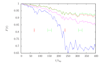
Figure 1: Fidelity as a function of time for single runs of Grover’s quantum search algorithm. Numerical simulations: without noise and exact (red line), using the near resonant approximation (green line); with static Larmor frequency noise ($\epsilon_{L}=0.02$) and exact (blue line), using the near resonant approximation (pink line). The red and green vertical bars indicate the position of pulses implementing the oracle (red bars) and the conditional reflection (green bars). Time is indicated in units of $t_{\rm hp}$ the duration of a $\pi/2$-pulse.

To start our study, we analyse single runs without any averaging. We compare calculations with and without noise, as well as exact calculations and calculations which apply the near resonant approximation. We use a quantum register of 3+1 qubits to simulate Grover’s search algorithm. The qubits are arranged according to the string xx.x, where x represents a data qubit, while the . represents the auxiliary qubit which is used to implement the oracle and the conditional reflection. The algorithm consists of an initial sequence of Hadamard gates $H^{(3)}$ followed by two Grover steps.

In the simulation for Fig. 1 the algorithm searches for the state 0 (string 00.0). On the graph we indicate the time intervals where the quantum oracle is implemented with red bars. These intervals therefore mark the start of a Grover step. Furthermore, we mark the time intervals where the conditional reflection is implemented with green bars. The red solid line shows the fidelity as a function of time for the exact calculation without noise. During the algorithm, the fidelity drops with more or less constant rate from $F(0)=1$ to $F_{\rm end}\approx 0.92$. This reminds us that the implementation of the quantum gates via RF-pulses as such already introduces errors. On the graph, time is indicated in units of $t_{\rm hp}$ the duration of a $\pi/2$-pulse (see end of Sec. 3). The green solid line shows the same calculation, but with the near resonant approximation being applied. It follows the exact calculation very well. The near resonant approximation neglects the far resonant, where the frequency missmatch is of the order of the Larmor frequencies. The fidelity is generally a bit larger than for the exact calculation. The agreement between the exact calculation and the near resonant approximation is completely lost as soon as the Larmor frequency noise (here it is static noise may be better described as random detunings) is switched on (blue and pink solid lines). The blue line shows the exact calculation for $\epsilon_{L}=0.02$ which only initially follows the curve for the fidelity decay without noise. More or less in the middle of the algorithm, the fidelity curve drops rather abruptly to a level of $F(t)\approx 0.7$, where it saturates. The near resonant approximation doesn’t show this behavior. Instead it stays close to the curve which shows the fidelity decay without noise. We may conclude that the noise introduces additional errors primarily via such indirect transitions which are neglected in the near resonant approximation. In the simulations shown, there is no indication that the oracle or the conditional reflection play any special role in the loss of fidelity.

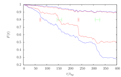
Figure 2: The average fidelity as a function of time in the case of static (red lines) and random (blue lines) Larmor frequency noise. Exact numerical simulations and the near resonant approximations are shown in the same color. The latter largely over-estimate the fidelity and fail to reproduce its true behaviour. Red and green vertical bars again indicate those time intervals, where the oracle and the conditional reflections are applied.

Figure 2 shows the average fidelity as described by Eq. (21) for static and random noise on the Larmor frequencies. The simulations are averaged over an ensemble of $n_{\rm rep}$ independent repetitions of the algorithm. In the case of the exact numerical simulations, $n_{\rm rep}=50$ (static noise) and $25$ (random noise). In the case of the near resonant approximations, $n_{\rm rep}=1000$ in both cases. This figure serves to demonstrate that the behavior of the fidelity may be very different for different repetitions – at least for static noise (compare with Fig. 1). We expect smaller variations within individual repetitions in the case of random noise, since there, the fidelity depends on a large number of random variables which tend to wash out any kind of extreme behavior. Interestingly, the simulations reveal that for static noise, fidelity is lost to a large extent during the oracle and the conditional reflection pulses. For random noise, the fidelity drop is more uniform. Finally, Fig. 2 again demonstrates the failure of the near resonant approximation in the presence of Larmor frequency noise.

Static vs. random Larmor frequency noise

Here, we analyse the average fidelity for the whole algorithm as a function of the noise amplitude. Averages are now taken over ensembles which contain typically about $n_{\rm rep}=100$ repetitions. The statistical error (due to the finite size of the ensemble) is estimated as follows: We divide the $n_{\rm p}$ fidelity values for each repetition into $p$ sub-ensembles of equal size. This yields average fidelities $F_{i},\,i=1,\ldots,p$. We take care that these sub-ensembles are sufficiently large such that the group-averaged fidelities are Gaussian distributed. That allows us to estimate the variance of the full average: $F=p^{-1}\sum_{i=1}^{p}F_{i}$ by calculating the best estimate for the variance of the group averages:

$${\rm var}(F)=\frac{1}{p}\;{\rm var}(F_{i})\;,\qquad{\rm var}(F_{i})=\frac{1}{p-1}\sum_{i=1}^{p}(F_{i}-F)^{2}\;.$$ (23)

We then use the standard deviation $\sigma(F)=\sqrt{{\rm var}(F)}$ as an estimate for our statistical error.

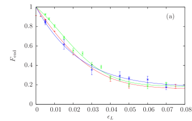
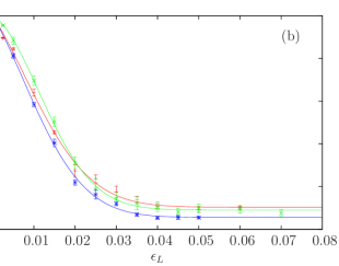
Figure 3: The fidelity $F_{\rm end}$ for static (a) and random (b) noise on the Larmor frequencies. Exact numerical simulations: $4$ qubits, target state $0$ (red error bars); $4$ qubits, target state $8$ (green error bars); $5$ qubits, target state $27$ (blue error bars). The solid lines of the corresponding colour show a phenomenological fit with Eq. (24) to the numerical data.

Fig. 3 shows the final average fidelity $F_{\rm end}$ of the whole algorithm as a function of the amplitude $\epsilon_{L}$ of the Larmor frequency noise. We compare the simulations with static noise (panel (a)) and random noise (panel (b)). In either case, we simulate the algorithm for four qubits and target states $0$ and $8$, and also for five qubits and the target state $27$. For a given noise model (static or random) the fidelity $F_{\rm end}$ behaves very similar in all cases. In panel (a) we observe a roughly exponential decrease for increasing $\epsilon_{L}$. At large values of $\epsilon_{L}$ the fidelity saturates at approximately $f_{\rm bas}\approx 0.175$. In panel (b), random noise, we observe a somewhat faster decay. Again the fidelity saturates for large $\epsilon_{L}$, but now the fidelity saturates earlier than in the case of static noise. Also, the saturation level is somewhat smaller: $f_{\rm bas}\approx 0.08$. To compare the behavior of the final fidelity $F_{\rm end}$ more quantitatively, we consider the following phenomenological model function:

$$f(\epsilon)=f_{\rm bas}+(1-f_{\rm bas})\;\exp\left[-(\epsilon/\epsilon_{2})^{2}-\epsilon/\epsilon_{1}\right]\;,$$ (24)

with the fit parameters $f_{\rm bas},\epsilon_{2}$, and $\epsilon_{1}$. In this parametrization, $\epsilon_{2}$ indicates the point where Gaussian decay becomes important. Similarly, $\epsilon_{1}$ indicates the point where exponential decay becomes important. For the three cases shown in Fig. 3(a), static noise, we obtain the following results:

$$\begin{array}[]{r|ccc}&f_{\rm bas}&\epsilon_{2}&\epsilon_{1}\\ \hline\cr\text{4 qubits, O(0)}&0.161(49)&0.046(20)&0.0315(73)\\ \text{4 qubits, O(8)}&0.186(19)&0.0359(40)&0.0510(80)\\ \text{5 qubits, O(27)}&0.178(62)&0.11(22)&0.0235(23)\end{array}\;,$$ (25)

where the statistical uncertainties of the fit values are given in parenthesis (they refer to the last two digits of the respective fit value). For the three cases shown in Fig. 3(b), dynamic noise, we obtain:

$$\begin{array}[]{r|lll}&f_{\rm bas}&\epsilon_{2}&\epsilon_{1}\\ \hline\cr\text{4 qubits, O(0)}&0.104(12)&0.0224(20)&0.0303(44)\\ \text{4 qubits, O(8)}&0.0904(45)&0.01870(55)&0.083(16)\\ \text{5 qubits, O(27)}&0.0555(83)&0.0209(14)&0.0291(34)\end{array}$$ (26)

Comparing the reduction of the fidelity for static and random noise, we find that random noise has a more destructive effect. This holds even at very small noise levels. This result may be surprising in view of opposite results in Refs. [19, 28]. However, note that both articles focus on larger quantum registers with more qubits and correspondingly more Grover steps. This is possible because they work with abstract gates and gate errors.

5.2 Rabi-frequency noise

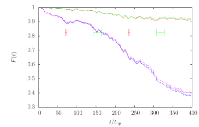
Figure 4: Fidelity as a function of time for single runs in the presence/absence of static Rabi frequency noise. Numerical simulations: without noise and exact (red line); using the near resonant approximation (green line); with noise, $\epsilon_{R}\xi=0.005$, and exact (blue line); using the near resonant approximation (pink line). Red and green vertical bars again indicate those time intervals, where the oracle and the conditional reflections are applied.

In this section we study the effects of amplitude noise on the RF-field. In the present approach this is equivalent to adding noise to the Rabi-frequency. As in the previous case, we consider static and dynamic noise. In the case of static noise, the fidelity depends on only one random variable, the detuning of the Rabi-frequency: $\Omega\to\Omega_{o}+\epsilon_{R}\xi$, where $\xi$ is a random Gaussian variable with zero mean and unit variance. This detuning of the Rabi frequency changes at random for each repetition, while being kept fixed during the execution of the algorithm. In the case of dynamic noise, the detuning changes at random for each microwave pulse. As in the case of Larmor frequency noise, we will first study the behavior of fidelity as a function of time and only afterwards the final fidelity (for the execution of the whole algorithm) as a function of the noise amplitude. We will find that the near resonant approximation is accurate in the presence of Rabi frequency noise. In the study of the final fidelity $F_{\rm end}$, we therefore use that approximation.

Fig. 4 shows the fidelity as a function of time for single runs of Grover’s search algorithm. We compare simulations with and without static Rabi frequency noise in analogy to Fig. 1, where we showed a similar figure for the case of static Larmor frequency noise. Here, a single run with static Rabi frequency noise, rather means that the simulation is performed with a certain detuning: $\epsilon_{R}\xi=0.005$. Comparing these results with those in Fig. 1, we find that a certain degree of fidelity loss requires a considerably larger amount of noise in the case of Larmor frequency noise ($\epsilon_{L}=0.02$). Furthermore, we observe that the near resonant approximation is very accurate in the present case of Rabi frequency detuning.

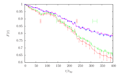
Figure 5: Average fidelity as a function of time for static and dynamic Rabi frequency noise with amplitude $\epsilon_{R}=0.005$. Numerical simulations: Static noise, exact (red line); near resonant approximation (green line). Dynamic noise, exact (blue line); near resonant approximation (pink line).

Fig. 5 shows the average fidelity for static (red line with error bars: exact numerical calculation; green line with error bars: near resonant approximation) and dynamic (blue line with error bars: exact numerical calculation; pink line with error bars: near resonant approximation) Rabi frequency noise. The error bars represent the estimate of the statistical error as explained in Eq. (23). The exact calculations are performed with $n_{\rm rep}=100$ repetitions, the near resonant approximations with $n_{\rm rep}=1000$. Note that the statistical uncertainty is quite large for static noise whereas it is very small for dynamic noise. Comparing to Fig. 2 we observe much less pronounced differences between oracle and conditional reflection on the one hand and the Hadammard gates on the other. In both cases, static and random noise, the difference between exact simulation and near resonant approximation is within the statistical error.

Static vs. Random Rabi frequency noise

From the results for the fidelity as a function of time, we saw that the near resonant approximation works very well in the case of Rabi frequency noise. Since it provides an enormous speed-up of the simulations, we will use it almost exclusively in the present section.

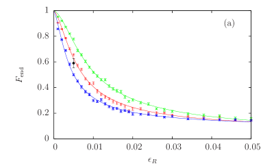
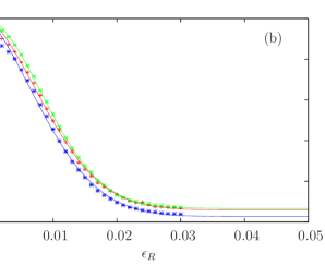
Figure 6: The fidelity $F_{\rm end}$ for static (a) and dynamic (b) Rabi frequency noise of strength $\epsilon_{R}$. Numerical simulations using the near resonant approximation: $4$ qubits, target state $0$ (red error bars); $4$ qubits, target state $8$ (green error bars); $5$ qubits, target state $27$ (blue error bars). The solid lines of the corresponding colour show the phenomenological fit with Eq. (27) (panel (a)) and Eq. (24) (panel b) to the numerical data. The black error bar near the red curve shows one case, where the fidelity has been calculated exactly (static noise, $4$ qubits, target state $0$).

Figure 6 shows the average fidelity $F_{\rm end}$ for the complete algorithm as a function of the amplitude $\epsilon_{R}$ of the Rabi frequency noise. In panel (a), we consider static noise, in panel (b), dynamic noise. We find a striking difference in the functional dependence of the fidelity between the two cases. For dynamic noise (panel (b)) we expect the fit function Eq (24) to work well. However in the case of static noise (panel (a)) we clearly need a different fit function to account for the apparently algebraic decay. In an attempt to maintain the general structure of the fit function as much as possible, we choose the new fit function of the form

$$g(\epsilon)=g_{\rm bas}+\frac{1-g_{\rm bas}}{\sqrt{(\epsilon/\epsilon_{2})^{2}+\epsilon/\epsilon_{1}+1}}\;.$$ (27)

The following two tables contain the results of the fits for static and dynamic Rabi frequency noise.

• Static noise: For the fit function $g(\epsilon)$ from Eq. (27) one obtains the following fit values for the three cases considered:

  $$\begin{array}[]{r|lll}&g_{\rm bas}&\epsilon_{2}&\epsilon_{1}\\ \hline\cr\text{4 qubits, O(0)}&0.052(10)&0.00429(23)&0.0140(45)\\ \text{4 qubits, O(8)}&0.0230(98)&0.00633(24)&0.032(10)\\ \text{5 qubits, O(27)}&0.0798(69)&0.00289(14)&0.0064(14)\end{array}$$ (28)

• Dynamic noise: Here, we use the same fit function $f(\epsilon)$ from Eq. (24) as in the case of Larmor frequency noise, and we obtained the following fit values:

  $$\begin{array}[]{r|lll}&f_{\rm bas}&\epsilon_{2}&\epsilon_{1}\\ \hline\cr\text{4 qubits, O(0)}&0.0589(62)&0.01437(44)&0.0352(31)\\ \text{4 qubits, O(8)}&0.0670(28)&0.01325(16)&0.0708(61)\\ \text{5 qubits, O(27)}&0.0267(89)&0.01499(72)&0.0254(23)\end{array}$$ (29)

The statistical uncertainties of the fit values are given in parenthesis. They refer to the last two digits of the respective fit value.

Finally, we may again ask which kind of noise, static or random, is leads to a larger loss of fidelity. While in Fig. 3 (Larmor frequency noise) it was the random noise, here in Fig. 6 the situation is more or less undecided. We note however that in the case of static noise (panal (a)) the different cases lead to a considerable spreading between the results in contrast to random noise (panel (b)), where the corresponding curves are very close together. We may also note that the $5$-qubit case in panel (a) shows initially the fastest drop in fidelity. It therefore has the correct tendency if we believe that for more qubits and more Grover steps, the static errors should lead to lower fidelities [19, 28].

Using the near resonant approximation, the numerical studies on Rabi frequency noise can be performed very efficiently. This would allow us to consider the Grover search algorithm in a larger quantum register with more qubits. We would need longer pulse sequences and more complex gate sequences for the implementation of the oracle. However, the main obstacle in considering more qubits are the unitary errors of our pulse sequence. Without additional error reduction (e.g. along the lines of Ref. [29]), the unitary errors alone would already reduce the final fidelity $F_{\rm end}$ so much that the effects of additional noise could not be analysed.

6 Conclusion

We studied the effect of noise on the performance of Grover’s search algorithm implemented on a nuclear spin quantum computer with four spins coupled via first- and second-neighbor Ising interactions. Starting from the ground state, the quantum search algorithm attempts to build-up the target state in the quantum register, using the information obtained from inquieries of a quantum oracle. We used the fidelity to quantify the effect of noise on the final state, i.e. the result of the algorithm. We considered different types of noise: (i) Noise affecting the Larmor frequencies which would be due to fluctuations in the static magnetic field, and (ii) noise affecting the Rabi frequency, which would be due to fluctuations in the intensity of the radio-frequency pulses. We simulate the noise by randomly detuning the respective frequencies from their nominal values. For both cases (i) and (ii) we considered two types of noise, systematic and random errors. In the case of systematic errors, the resepective frequencies are randomly chosen at the beginning of the algorithm and then kept fixed during the whole protocol. By contrast, in the case of random errors, the respective frequencies are randomly chosen for each radiofrequency pulse.

We found that the threshold of this amplitude for still having good performance of the algorithm is $\epsilon_{L}\leq 0.005$ for Larmor-frequency noise and $\epsilon_{R}\leq 0.1$ for systematic error on Rabi-frequency .We also found that this algorithm is much more sensitive to systematic errors than random errors which behave like an exponential and Gaussian decay respectively. One may say that this Gaussian behavior corresponds to the robustness of the algorithm. As we mentioned before, computing time increases very much with the number of qubits, making the increasing of the number of Grover steps not feasible within our model.

References

- [1] Grover L K 1997 Phys. Rev. Lett. 79 325
- [2] Grover L K 1998 Phys. Rev. Lett. 80 4329
- [3] Terhal B M and Smolin J A 1998 Phys. Rev. A 58 1822
- [4] Brassard G, Hoyer P and Tapp A 1998 Automata Language and Programming, vol. 1443, Eds. Larsen K G, Skyum S and Winskel G (Berlin, Springer-Verlag)
- [5] Cerf N J, Grover L K and Williams C P 2000 Phys. Rev. A 61 032303
- [6] Gingrich R M, Williams C P and Cerf N J 2000 Phys. Rev. A 61 052313
- [7] Carlini A and Hosoya A 2001 Phys. Rev. A 280 114
- [8] Yang W L, Chen C Y and Feng M 2007 Phys. Rev. A 76 054301
- [9] Chuang I L, Gershenfeld N and Kubinec M 1998 Phys. Rev. Lett. 80 3408
- [10] Jones J A Mosca M and Hansen R H 1998 Nature 393 344
- [11] Kwiat P G, Mitchel J R, Schwindt P D D and White A G 2000 J. Mod. Optics 47 257
- [12] Long G L, Yan H Y, Li Y S, Tu C C, Tao J X, Chen H M, Liu M L, Zhang X, Luo J, Xiao L and Zeng X Z 2001 Phys. Lett. A 286 121
- [13] López G V, Gorin T and Lara L 2008 J. Phys. B 41 055504
- [14] López G V and Lara L 2005 J. Phys. B 38 3897
- [15] Berman G P, Kamenev D I, Doolen D D, López G V and Tsifrinovich V I 2002 Contemp. Math. 305 13
- [16] Berman G P, Doolen D D, López G V and Tsifrinovich V I 2000 Phys. Rev. A 61 062305
- [17] López G V, Gorin T and Lara L 2008 Int. J. Theo. Phys. 47 1641
- [18] Pablo-Norman B and Ruiz-Altaba M 1999 Phys. Rev. A 61 012301
- [19] Long G L, Li Y S, Zhang W L and Tu Ch C 2000 Phys. Rev. A 61 042305
- [20] Ellinas D and Konstadakis Ch 2001 arXiv: quant-ph/0110010v1
- [21] Song P H and Kim I 2003 Eur. Phys. J. D 23 299
- [22] Salas P. J. 2008 Eur. Phys. J. D 46 365
- [23] Zhirov O V and Shepelyansky D L 2006 Eur. Phys. J. D 38 405
- [24] Peres A 1984 Phys. Rev. A 30 1610
- [25] Gorin T, Prosen T, Seligman T H and Žnidarič M 2006 Phys. Rep. 435 33
- [26] Nielsen M A and Chuang I L 2000 Quantum Computation and Quantum Information (Cambridge, Cambridge University Press)
- [27] Long G L 2001 Phys. Rev. A 64 022307
- [28] Frahm K M, Fleckinger R and Shepelyansky D L 2004 Eur. Phys. J. D 29 139
- [29] Berman G P, Kamenev D I, Kassman R B, Pineda C and Tsifrinovich V I arXiv:quant-ph/0212070v1