Numerical Evaluation of Gauge Invariants for
$a$-Gauge Solutions in Open String Field Theory

Abstract

We evaluate gauge invariants (vacuum energy and gauge invariant overlap) for numerical classical solutions in the cubic open string field theory under Asano and Kato’s $a$-gauge fixing condition. We propose an efficient iterative procedure for solving the equations of motion so that the BRST invariance of the solutions is numerically ensured. The resulting gauge invariants are numerically stable and almost equal to those of Schnabl’s tachyon vacuum solution in the well-defined region of a gauge parameter. These results provide further evidence that the numerical and analytical solutions are gauge-equivalent.

1 Introduction

The cubic bosonic open string field theory (SFT)[1] has classical solutions that are expected to be a tachyon vacuum solution conjectured by Sen [2, 3, 4]. One of them is given as a numerical solution using a level truncation scheme in the Siegel gauge [5, 6, 7] and then an analytic solution is constructed in the Schnabl gauge,[8] which is a modified version of the Siegel gauge. These two solutions are believed to be the same tachyon vacuum solution. Although it is difficult to prove their equivalence by constructing an explicit gauge transformation between them, we can provide evidence using three gauge invariant quantities. First, we can find that these two solutions have almost the same values for two gauge invariants: one of these invariants is a vacuum energy[8] that should precisely cancel the D-brane tension and the other is a gauge invariant overlap[9, 10] that corresponds to the coupling of an open string field to an on-shell closed string. The third gauge invariant is an on-shell scattering amplitude in the SFT expanded around the tachyon vacuum. It should exactly vanish since the analytic solution gives a trivial cohomology of the kinetic operator around the vacuum[11]. The numerical solution has a similar tendency to provide vanishing scattering amplitudes[12, 13]. These are results consistent with the expectation that the analytic and numerical solutions are equivalent up to gauge transformation.

The purpose of this study is to provide further evidence of the gauge equivalence of the two solutions by the numerical calculation of the vacuum energy and gauge invariant overlap. In our calculation, we will truncate the level of the string field and fix it in Asano and Kato’s $a$-gauge[14, 15].

The “$a$-gauge” was proposed as a family of gauges with one-parameter $a$, which corresponds to the covariant gauge in the conventional gauge theory. It includes the Feynman-Siegel gauge ($a=0$) and Landau gauge ($a=\infty$). In SFT under $a$-gauge fixing condition, it was proved that on-shell physical amplitudes are gauge-independent[14]. The $a$-gauge condition is also applicable to the numerical analysis of the tachyon vacuum using the level truncation scheme[16]. The potential in the $a$-gauge has a nontrivial local minimum where the energy density approximately equals that of the tachyon vacuum. In other words, the nontrivial vacuum energy remains almost the same as that of the Siegel gauge for various values of $a$. Although the $a$-gauge yields good results in level truncation analysis, the BRST invariance of the vacuum[17] has not yet been evaluated and it must be checked to confirm that the vacuum is truly physical. In this study, we will perform a numerical test on the BRST invariance, or the validity of the classical equations of motion, for the nontrivial vacuum in the $a$-gauge.

The gauge invariant overlap is an interesting quantity since it takes nontrivial values for the nonperturbative vacuum[9, 10]. Moreover, from the intensive study of the overlap, we have new insights into the relation among the tachyon vacuum solution and boundary states[18, 19, 20]. In this paper, we will numerically calculate the gauge invariant overlap for the nontrivial solution in the $a$-gauge, and we will confirm that it is also in good agreement with the Siegel gauge result. This will also confirm the gauge equivalence between the numerical and analytical solutions.

First, we will discuss the string field theory and the equations of motion focusing on the $a$-gauge fixing condition in §2. In §3, we will discuss an iterative algorithm solving the equations of motion. We will propose a new algorithm that simplifies numerical computations in the $a$-gauge. The numerical results will be provided in §4 and then we will give a summary and discussion in §5. In Appendix A, we will define a norm of string fields. In Appendix B, we will give samples of numerical data corresponding to plots in §4.

2 Equations of motion in various gauges

In cubic bosonic open SFT[1], the gauge-invariant action is given by

$$S[\Psi]=-\frac{1}{g^{2}}\int\left(\frac{1}{2}\Psi*Q_{\rm B}\Psi+\frac{1}{3}\Psi*\Psi*\Psi\right),$$ (1)

where the string field $\Psi$ is expanded by string Fock space states with the ghost number $1$. The action is invariant under the infinitesimal gauge transformation

$$\delta\Psi=Q_{\rm B}\Lambda+\Psi*\Lambda-\Lambda*\Psi.$$ (2)

From the least-action principle, the equation of motion is derived as

$$Q_{\rm B}\Psi+\Psi*\Psi=0.$$ (3)

We impose a gauge fixing condition to solve the equations of motion. Let us consider the linear gauge fixing condition [14] for some operator ${\cal O}_{\rm GF}$,

$${\cal O}_{\rm GF}\Psi=0.$$ (4)

It provides the Siegel gauge if $b_{0}$ is taken as ${\cal O}_{\rm GF}$. The $a$-gauge fixing condition[15] is defined by the operator

$${\cal O}_{\rm GF}=b_{0}M+ab_{0}c_{0}\tilde{Q},$$ (5)

where $a$ denotes the gauge parameter and the operators $M$ and $\tilde{Q}$ are defined by the expansion of the BRST charge with respect to ghost zero modes,

$$Q_{\rm B}=\tilde{Q}+c_{0}L_{0}+b_{0}M.$$ (6)

The $a$-gauge at $a=0$ is proved to be equivalent to the Siegel gauge, though the operator ${\cal O}_{\rm GF}$ is different from $b_{0}$. In the infinite $a$ limit, the $a$-gauge represents the Landau gauge for a massless vector field. The Landau gauge can be also given by the regular operator

$${\cal O}_{\rm GF}=b_{0}c_{0}\tilde{Q}.$$ (7)

Let us consider classical solutions of the equation of motion (3) under the gauge fixing condition (4). First, we introduce the undetermined multiplier string field ${\cal B}$ with a ghost number $2-{\rm gh}({\cal O}_{\rm GF})$, where ${\rm gh}(A)$ denotes the ghost number of $A$, into the action:

$$S[\Psi,{\cal B}]=-\frac{1}{g^{2}}\int\left(\frac{1}{2}\Psi*Q_{\rm B}\Psi+\frac{1}{3}\Psi*\Psi*\Psi\right)+\int{\cal B}*{\cal O}_{\rm GF}\Psi.$$ (8)

The equations of motion are derived as

$${\cal O}_{\rm GF}\Psi=0,$$ (9)

$$Q_{\rm B}\Psi+\Psi*\Psi=g^{2}\,{\rm bpz}({\cal O}_{\rm GF}){\cal B},$$ (10)

where ${\rm bpz}({\cal O})$ denotes the BPZ conjugation of some operator ${\cal O}$.

If we find a projection operator ${\cal P}_{\rm GF}$ corresponding to the gauge condition (9), such as

$${\cal P}_{\rm GF}^{2}|F\rangle_{1}={\cal P}_{\rm GF}|F\rangle_{1},~{}~{}~{}~{}{\cal O}_{\rm GF}{\cal P}_{\rm GF}|F\rangle_{1}=0,$$ (11)

for any state $|F\rangle_{1}$ with ${\rm gh}(|F\rangle_{1})=1$, we obtain

$${\rm bpz}({\cal P}_{\rm GF})\left(Q_{\rm B}\Psi+\Psi*\Psi\right)=0$$ (12)

from Eq. (10). This equation represents part of the gauge unfixed equation of motion (3). For the Siegel gauge condition, the operator ${\cal P}_{\rm GF}$ is given by $b_{0}c_{0}$.

The projection ${\cal P}_{\rm GF}$ for the $a$-gauge Eq. (5) is given by[15]

$${\cal P}_{\rm GF}=1+\frac{1}{a-1}\Bigl{(}\frac{\tilde{Q}}{L_{0}}+c_{0}\Bigr{)}(b_{0}+ab_{0}c_{0}W_{1}\tilde{Q}),$$ (13)

where we consider $L_{0}\neq 0$ sector and $a\neq 1$. The operator $W_{1}$ is given by

$$W_{1}=\sum_{i=0}^{\infty}\frac{(-1)^{i}}{\{(i+1)!\}^{2}}M^{i}(M^{-})^{i+1},~{}~{}M^{-}=-\sum_{n=1}^{\infty}\frac{1}{2n}b_{-n}b_{n}.$$ (14)

Using $\tilde{Q}^{2}=-L_{0}M$ and the relations[15, 14]

$${\rm bpz}(W_{1})b_{0}c_{0}|F\rangle_{2}=-W_{1}b_{0}c_{0}|F\rangle_{2},~{}~{}~{}~{}{\rm bpz}(W_{1})c_{0}b_{0}|F\rangle_{3}=-W_{1}c_{0}b_{0}|F\rangle_{3}\,,$$ (15)

$$MW_{1}b_{0}c_{0}|F\rangle_{2}=b_{0}c_{0}|F\rangle_{2},~{}~{}~{}~{}~{}~{}~{}~{}~{}~{}MW_{1}c_{0}b_{0}|F\rangle_{3}=c_{0}b_{0}|F\rangle_{3},$$ (16)

$$W_{1}Mb_{0}c_{0}|F\rangle_{0}=b_{0}c_{0}|F\rangle_{0},~{}~{}~{}~{}~{}~{}~{}~{}~{}~{}W_{1}Mc_{0}b_{0}|F\rangle_{1}=c_{0}b_{0}|F\rangle_{1},$$ (17)

for any state $|F\rangle_{n}$ with ${\rm gh}(|F\rangle_{n})=n$, we can derive Eq. (11).

3 Iterative procedure in various gauges

Gaiotto and Rastelli[7] pointed out that, in the Siegel gauge, an efficient numerical approach to solving the equations of motion is Newton’s method. As they noted, the iterative algorithm can be expressed in the compact form

$$\Psi_{(n+1)}=Q_{\Psi_{(n)}}^{-1}(\Psi_{(n)}*\Psi_{(n)})$$ (18)

for $n=0,1,2,\cdots$ with an initial value $\Psi_{(0)}$. Here, the operator $Q_{\Psi}^{-1}$ is defined by

$$b_{0}Q_{\Psi}^{-1}|F\rangle_{2}=0,$$ (19)

$$c_{0}b_{0}\left(Q_{\Psi}Q_{\Psi}^{-1}|F\rangle_{2}-|F\rangle_{2}\right)=0$$ (20)

for any ghost number two state $|F\rangle_{2}$, where

$$Q_{\Psi}\Phi=Q_{\rm B}\Phi+\Psi*\Phi+\Phi*\Psi$$ (21)

for any ghost number one string field $\Phi$. Eq. (19) corresponds to the Siegel gauge condition and Eq. (20) implies that $Q_{\Psi}^{-1}$ is an inverse operator of $Q_{\Psi}$ in a sense.

Noting the above definition, if we get an $n$-th configuration $\Psi_{(n)}$, we can construct an $(n+1)$-th configuration $\Psi_{(n+1)}$ by solving the linear equations

$$b_{0}\Psi_{(n+1)}=0,$$ (22)

$$c_{0}b_{0}\left(Q_{\Psi_{(n)}}\Psi_{(n+1)}-\Psi_{(n)}*\Psi_{(n)}\right)=0.$$ (23)

Suppose that we find a converged configuration $\Psi_{(\infty)}$ after the infinite iterative process of Eq. (18). By Eqs. (22) and (23), we can find that the obtained $\Psi_{(\infty)}$ satisfies the Siegel gauge condition $b_{0}\Psi_{(\infty)}=0$ and

$$c_{0}b_{0}(Q_{\rm B}\Psi_{(\infty)}+\Psi_{(\infty)}*\Psi_{(\infty)})=0.$$ (24)

This is a projected part of the whole equation of motion (3), which is equivalent to Eq. (12) with ${\cal P}_{\rm GF}=b_{0}c_{0}$ in the Siegel gauge.

Now, let us look for the iterative algorithm applied to the $a$-gauge condition. To do that, we have only to generalize the linear equations (22) and (23) straightforwardly using ${\cal O}_{\rm GF}$ given by Eq. (5) (or Eq. (7) for $a=\infty$) and ${\cal P}_{\rm GF}$ given by Eq. (13):

$${\cal O}_{\rm GF}\Psi_{(n+1)}=0,$$ (25)

$${\rm bpz}({\cal P}_{\rm GF})\left(Q_{\Psi_{(n)}}\Psi_{(n+1)}-\Psi_{(n)}*\Psi_{(n)}\right)=0.$$ (26)

Actually, we can find a numerically converged solution through this algorithm with the initial configuration given in Eq. (32) using the level truncation. We can also obtain the same configuration by solving the equation of motion for the gauge fixed action: $S[\Psi]|_{{\cal O}_{\rm GF}\Psi=0}$, which is equivalent to Eq. (12) with Eq. (13), using the level truncation.

However, Eq. (26) is so complicated that the computational speed may be lower than that in the Siegel gauge case, Eq. (23). Since the operators $\tilde{Q}$ and $W_{1}$ in the projection operator include an infinite sum of ghost modes, it is a very cumbersome procedure to act these on a state. As an alternative, let us consider the equations

$${\cal O}_{\rm GF}\Psi_{(n+1)}=0,$$ (27)

$$c_{0}b_{0}\left(Q_{\Psi_{(n)}}\Psi_{(n+1)}-\Psi_{(n)}*\Psi_{(n)}\right)=0,$$ (28)

where the projection operator ${\cal P}_{\rm GF}$ (13) is replaced with the simple operator $b_{0}c_{0}$. From Eqs. (27) and (28), a converged configuration $\Psi_{(\infty)}$ after infinite iterations satisfies

$${\cal O}_{\rm GF}\Psi_{(\infty)}=0,$$ (29)

$$c_{0}b_{0}\left(Q_{\rm B}\Psi_{(\infty)}+\Psi_{(\infty)}*\Psi_{(\infty)}\right)=0.$$ (30)

Eq. (29) imposes that $\Psi_{(\infty)}$ is in the $a$-gauge subspace, but Eq. (30) is the same as the equation of motion under the Siegel gauge condition (24). This mismatch in the gauge fixing condition (except in the case $a=0$, which is equivalent to the Siegel gauge) seems to suggest that we cannot find a solution in the $a$-gauge by solving Eqs. (27) and (28).

Generically, the classical solution should satisfy all of the equations of motion, included in Eq. (3). In the case of the Siegel gauge, $\Psi_{(\infty)}$ obeys Eq. (24), which is a projected part of Eq. (3). It can be used for finding the classical solution. However the unprojected equations should be satisfied by $\Psi_{(\infty)}$ to ensure that the solution is a true vacuum. Actually, the remaining equation $b_{0}c_{0}\left(Q_{\rm B}\Psi_{(\infty)}+\Psi_{(\infty)}*\Psi_{(\infty)}\right)=0$ indicates the BRST invariance of the classical solution and it holds to a high accuracy for the numerical solution in the Siegel gauge.[17, 7]

Therefore, $\Psi_{(\infty)}$ in Eq. (30) is a possible candidate for the solution in the $a$-gauge because it satisfies the $a$-gauge condition and part of all the equations of motion. To verify whether it is a true solution, we will check the remaining part:

$$b_{0}c_{0}\left(Q_{\rm B}\Psi_{(\infty)}+\Psi_{(\infty)}*\Psi_{(\infty)}\right)=0,$$ (31)

apart from projected equation of motion (30). Thus, we are able to find the numerical solution more efficiently by using the simplified equations Eqs. (27) and (28).

4 Level-truncated solutions

When applying the algorithm in the previous section, namely, Eqs. (27) and (28), to find a solution, we have to specify an initial configuration $\Psi_{(0)}$. We take it as

$$\Psi_{(0)}=\frac{64}{81\sqrt{3}}\,c_{1}\left|0\right>,$$ (32)

which is the nontrivial solution for the level $(0,0)$ truncation. To proceed with the iteration numerically, we use the level truncation approximation corresponding to the $(L,2L)$ and $(L,3L)$ truncations. Namely, we truncate the string field to level $L\equiv L_{0}+1$ and interaction terms, which appear in the star product, up to total level $2L$ or $3L$. To terminate the iteration, we should specify the accuracy limit of convergence. We define a “norm” of a string field $\|\cdot\|$ as in Appendix A to measure the accuracy. We terminate the iterative procedure if the relative error reaches

$$\frac{\|\Psi_{(n+1)}-\Psi_{(n)}\|}{\|\Psi_{(n)}\|}<10^{-8}.$$ (33)

For all levels of $L$ and various values of $a$, the $n$-th configuration reaches this accuracy limit after 10 iteration steps or less. At the same time, we explicitly examine whether the resulting solution satisfies Eq. (30) by calculating the quantity

$$\frac{\|c_{0}b_{0}(Q_{\rm B}\Psi_{(n)}+\Psi_{(n)}*\Psi_{(n)})\|}{\|\Psi_{(n)}\|}.$$ (34)

We verified that this quantity is smaller than $10^{-8}$ for the resulting solution which satisfies the accuracy limit Eq. (33).

4.1 Evaluation of gauge invariants

The resulting solution obtained by the iteration above depends on the gauge parameter. For the solution $\Psi_{a}$, we calculate the classical action

$$S(\Psi_{a})=-2\pi^{2}\left(\frac{1}{2}\left<\Psi_{a},\,Q_{\rm B}\Psi_{a}\right>+\frac{1}{3}\left<\Psi_{a},\,\Psi_{a}*\Psi_{a}\right>\right),$$ (35)

which is normalized to be one for the Schnabl solution. In Fig. 1, we show plots of vacuum energy for $(L,2L)$ truncation as a function of $a$.

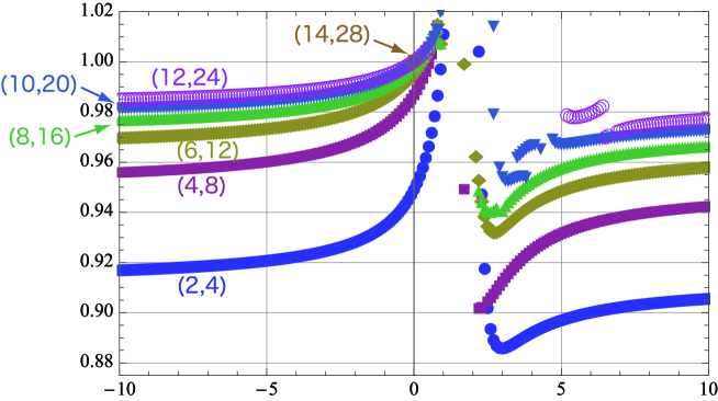
Figure 1: Plots of vacuum energy $S(\Psi_{a})$ for $(L,2L)$ truncation. The horizontal axis denotes the value of the gauge parameter $a$. (We have only one datum for $(14,28)$ truncation, which is in the Siegel gauge $(a=0)$. For other $a$-gauges ($a\neq 0$), calculations are harder in our Mathematica program.)

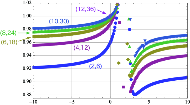
Figure 2: Plots of vacuum energy $S(\Psi_{a})$ for $(L,3L)$ truncation. The horizontal axis denotes the value of the gauge parameter $a$. (We have only one datum for $(12,36)$ truncation, which is in the Siegel gauge $(a=0)$.)

In the region at approximately $a=1$, the value of the action is unstable for every level. This instability was reported to occur for level 2, 4 and 6 analyses in an earlier paper[16]. According to the paper, $a=1$ is a gauge nonfixed point in the free theory and then the nearby gauge horizon seems to remain at approximately $a=1$ if the interaction is switched on. The plots in Fig. 1 suggest that the situation would not improve despite higher-level calculation.

In the well-defined region except the dangerous zone at approximately $a=1$, the value of the action is stable at over 90% of the expected value for the tachyon vacuum. Moreover, the value gradually approaches $1$ as truncation level is increased. These are good results, which are consistent with the gauge independence of vacuum energy. The same tendency is found in the level $(L,3L)$ calculation, as depicted in Fig. 2.

Now, let us consider the gauge invariant overlap for the numerical solution. The gauge invariant overlap is defined by

$${\cal O}_{V}(\Psi)=\left<{\cal I}\right|V(i)\left|\Psi\right>,$$ (36)

where ${\cal I}$ denotes the identity string field, and $V(i)$ corresponds to an on-shell closed string vertex operator. Hereafter, the overlap is normalized so that it equals $1$ for the Schnabl tachyon vacuum solution. Figs. 3 and 4 show plots of the gauge invariant overlap against $a$ for level $(L,2L)$ and $(L,3L)$ truncations. As in the case of the action, the plots are almost gauge-independent in the well-defined region of the gauge parameter $a$. As truncation level is increased, the stable value of the overlap approaches the expected value of $1$. These results suggest that the numerical value of the overlap is physically reliable.

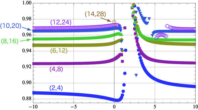
Figure 3: Plots of gauge invariant overlap ${\cal O}_{V}(\Psi_{a})$ for $(L,2L)$ truncation. The horizontal axis denotes the value of the gauge parameter $a$. (We have only one datum for $(14,28)$ truncation, which is in the Siegel gauge $(a=0)$.)

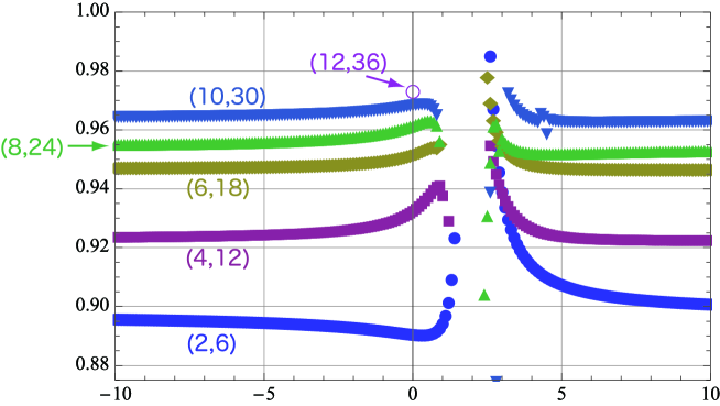
Figure 4: Plots of gauge invariant overlap ${\cal O}_{V}(\Psi_{a})$ for $(L,3L)$ truncation. The horizontal axis denotes the value of the gauge parameter $a$. (We have only one datum for $(12,36)$ truncation, which is in the Siegel gauge $(a=0)$.)

Here, we display graphs of the action and overlap for various $a$ in Figs. 5 and 6. The point $(1,1)$ is the result for Schnabl’s analytic solution and these figures clearly indicate that the numerical result from higher-level calculation is closer to the analytic result for various gauge parameters.

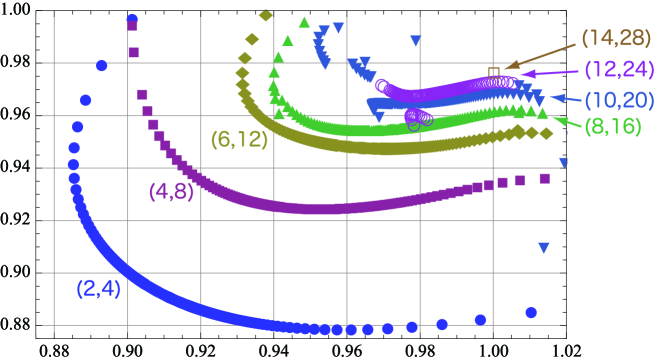
Figure 5: Plots of gauge invariants for $(L,2L)$ truncation. The horizontal axis denotes the action $S(\Psi_{a})$ and the vertical one denotes the gauge invariant overlap ${\cal O}_{V}(\Psi_{a})$. Each point denotes the value of $(S(\Psi_{a}),{\cal O}_{V}(\Psi_{a}))$ for various $a$ values. The left part of the “curve” for each level corresponds to $4\lesssim a<+\infty$ and the right part corresponds to $-\infty<a\lesssim 1/2$. The plots for $a\to+\infty$ and $a\to-\infty$ are continuously connected at that of the Landau gauge ($a=\infty$).

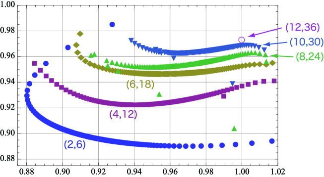
Figure 6: Plots of gauge invariants for $(L,3L)$ truncation. The horizontal axis denotes the action $S(\Psi_{a})$ and the vertical one denotes the gauge invariant overlap ${\cal O}_{V}(\Psi_{a})$. The tendency of the plots is similar to that of the $(L,2L)$ truncation in Fig. 5.

4.2 The validity of the equation of motion

Finally, we consider the remaining part of the equations of motion (31) for the resulting solution $\Psi_{a}$. To check it, let us consider the coefficient of $c_{-2}c_{1}|0\rangle$, which is the lowest-level state included on the left-hand side of Eq. (31). We plot it in Fig. 7 for the $(L,2L)$ truncation and in Fig. 8 for the $(L,3L)$ truncation. Both of them imply that the coefficient approaches zero at a higher level except in the dangerous zone at approximately $a=1$. We find that other coefficients on the left-hand side of Eq. (31) also approach zero at a higher level.

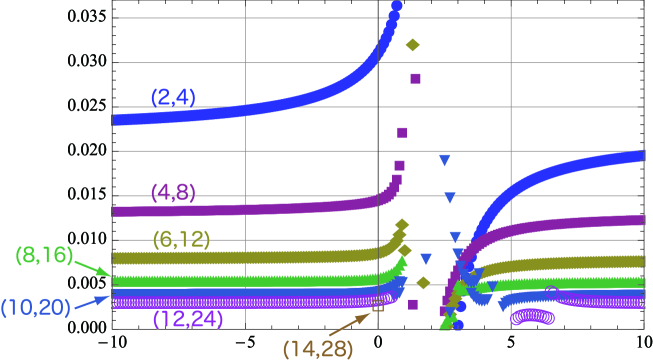
Figure 7: Plots of coefficient of $c_{-2}c_{1}|0\rangle$ on the left-hand side of Eq. (31) for $(L,2L)$ truncation. The horizontal axis denotes $a$.

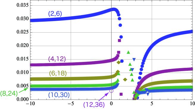
Figure 8: Plots of coefficient of $c_{-2}c_{1}|0\rangle$ on the left-hand side of (31) for $(L,3L)$ truncation. The horizontal axis denotes $a$.

In order to check all coefficients at one time, we compute

$$\frac{\|b_{0}c_{0}(Q_{\rm B}\Psi_{a}+\Psi_{a}*\Psi_{a})\|}{\|\Psi_{a}\|}.$$ (37)

This quantity is almost the same as $\|Q_{\rm B}\Psi_{a}+\Psi_{a}*\Psi_{a}\|/\|\Psi_{a}\|$ because Eq. (34) is negligible as mentioned earlier. We observe that $\|\Psi_{a}\|$ is within $0.56\sim 0.7$. Therefore, Eq. (37) can be used to measure the validity of all the equations of motion. We display the plots of Eq. (37) for various $a$ values in Figs. 9 and 10. Similarly, these plots are numerically stable in the well-defined region of the gauge parameter. We find that the norm approaches zero as the level is increased. Thus, the numerical solutions to Eq. (30) in the $a$-gauges constructed using Eqs. (27), (28) and (32) are the solutions to the equation of motion (3) to a good accuracy.

Here, we should comment on the computational method using the iterative equations Eqs. (25) and (26) with Eq. (32). Based on these equations, we can also find numerical solutions for various values of the gauge parameter $a$. The action and overlap for the solutions take numerical values around those of the analytic result for Schnabl’s solution. However, except that in the Siegel gauge case ($a=0$), the norm of all the equations of motion increases for a higher level. This suggests that the resulting solutions become worse as truncation level increases. Therefore, we emphasize that the iterative procedure based on Eqs. (27) and (28) has a significant advantage in that the resulting solutions numerically improve the accuracy of the equation of motion with respect to its norm.

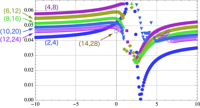
Figure 9: Plots of (37) for $(L,2L)$ truncation. The horizontal axis denotes $a$. For a fixed $a$, the value of Eq. (37) decreases with increasing level except for the $(2,4)$-truncation.

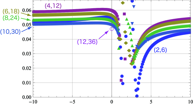
Figure 10: Plots of (37) for $(L,3L)$ truncation. The horizontal axis denotes $a$. For a fixed $a$, the value of Eq. (37) decreases with increasing level except for the $(2,6)$-truncation.

5 Concluding remarks

We have evaluated gauge invariants (action and gauge invariant overlap) for numerical solutions in the $a$-gauge by level truncation approximation. We have checked the validity of the equation of motion for the solutions. In the well-defined region of the gauge parameter $a$, the resulting gauge invariants are numerically equal to those of Schnabl’s tachyon vacuum solution. This provides evidence that previous numerical results in the Siegel gauge are gauge-independent and thus are physically correct. The results are consistent with the expectation that these solutions in the $a$-gauge are gauge-equivalent to Schnabl’s solution and represent a unique nonperturbative vacuum in bosonic open SFT.

The iterative procedure used in this study to solve the equations of motion is an efficient algorithm in the $a$-gauge. The algorithm simplifies linear equations in the $a$-gauge and achieves a reliable accuracy of the equation of motion with respect to its norm, which is nearly equal to that of the Siegel gauge. It would be interesting to determine why our algorithm is better than the conventional calculation method.

In this study, we used a norm with respect to a particular basis in order to measure the validity of the equation of motion. However, the norm convergence for a large $L$ limit might be a very strict condition in the level truncation approximation. It may be important to investigate the higher-level dependence of numerical solutions extensively, which will shed some light on good regularizations of string fields.

Appendix A Norm of String Fields

Here, we define a norm of string fields to investigate the accuracy of convergence of the iteration Eq. (33) and the validity of the equations of motion, Eqs. (34) and (37), numerically. Noting that ${\cal O}_{\rm GF}$ Eq. (5) (or Eq. (7) for $a=\infty$), which specifies the $a$-gauge condition, is made of the matter Virasoro modes $L_{n}^{({\rm m})}$ and $bc$-ghost modes only and commutes with $L_{0}$, we can restrict string fields to twist even universal space to proceed with the iterations of Eqs. (27) and (28) (or (26)) with the initial configuration Eq. (32).

The universal space is spanned by the states whose matter sector is of the form:

$$L^{({\rm m})}_{-n_{1}}L^{({\rm m})}_{-n_{2}}\cdots L^{({\rm m})}_{-n_{q}}|0\rangle_{\rm m}.~{}~{}~{}~{}(n_{1}\geq n_{2}\geq\cdots\geq n_{q}\geq 2)$$ (38)

We take an orthonormalized basis with respect to the BPZ inner product in the matter sector such as

$$\langle\varphi_{k,m_{k}},\varphi_{k^{\prime},m^{\prime}_{k^{\prime}}}\rangle=(-1)^{k}\delta_{k,k^{\prime}}\delta_{m_{k},m^{\prime}_{k^{\prime}}},~{}~{}~{}~{}~{}L_{0}^{({\rm m})}|\varphi_{k,m_{k}}\rangle=k|\varphi_{k,m_{k}}\rangle,$$ (39)

which is given by appropriate linear combinations of (38). In the ghost sector, we take a basis such as

$$|\psi_{k,m_{k}}\rangle=b_{-p_{1}}b_{-p_{2}}\cdots b_{-p_{r}}c_{-q_{1}}c_{-q_{2}}\cdots c_{-q_{s}}c_{1}|0\rangle_{\rm gh},$$ (40)

$$p_{1}>p_{2}>\cdots>p_{r}\geq 1,~{}~{}q_{1}>q_{2}>\cdots>q_{s}\geq 0,~{}~{}\sum_{t=1}^{r}p_{t}+\sum_{u=1}^{s}q_{u}=k.$$ (41)

Namely, our basis for twist even universal space is of the form $\varphi_{k,m_{k}}\otimes\psi_{l,n_{l}}$ whose level $k+l$ is even. In the level $(L,2L)$ or $(L,3L)$ truncation, string fields $\Phi$ can be expanded as

$$\Phi=\sum_{k+l\leq L}\sum_{m_{k},n_{l}}t_{k,m_{k};l,n_{l}}\,\varphi_{k,m_{k}}\otimes\psi_{l,n_{l}}.$$ (42)

Using this expansion, we define its norm $\|\Phi\|$ as

$$\|\Phi\|=\left(\sum_{k,m_{k},l,n_{l}}|t_{k,m_{k};l,n_{l}}|^{2}\right)^{\frac{1}{2}}.$$ (43)

Appendix B Samples of Numerical Data

In the following, we give some data of our numerical computation with level truncation.

Table 1: Vacuum energy $S(\Psi_{a})$ for $(L,2L)$ truncation. At $a=4$, the iteration for at least 10 steps does not converge for $(12,24)$-truncation. For $(14,28)$ truncation, we computed the configuration for $a=0$ only. In the case of the Siegel gauge $(a=0)$, we reproduced the data in Ref. Gaiotto:2002wy up to $L=14$.

$L$	$a=\infty$	$a=4$	$a=0.5$	$a=0$	$a=-2$
2	0.911461	0.891405	0.965684	0.948553	0.927610
4	0.949735	0.924272	0.998777	0.986403	0.967567
6	0.964287	0.942319	1.00432	0.994773	0.979586
8	0.972147	0.951844	1.00541	0.997780	0.985337
10	0.977517	0.966292	1.00550	0.999116	0.988741
12	0.981390	–	1.00531	0.999791	0.991016
14	–	–	–	1.00016	–

Table 2: Vacuum energy $S(\Psi_{a})$ for $(L,3L)$ truncation. For the $(12,36)$ truncation, we computed the configuration for $a=0$ only. In the case of the Siegel gauge $(a=0)$, we reproduced the data in Ref. Gaiotto:2002wy up to $L=12$. The data for $a\neq 0$ obtained using Eq. (28) are not the same as those in Ref. Asano:2006hm, which can be obtained using Eq. (26).

$L$	$a=\infty$	$a=4$	$a=0.5$	$a=0$	$a=-2$
2	0.914683	0.886606	0.977278	0.959377	0.935227
4	0.948672	0.916240	1.00007	0.987822	0.968273
6	0.962778	0.933562	1.00434	0.995177	0.979674
8	0.970986	0.944420	1.00527	0.997930	0.985329
10	0.976504	0.952494	1.00534	0.999182	0.988719
12	–	–	–	0.999822	–

Table 3: Gauge invariant overlap ${\cal O}_{V}(\Psi_{a})$ for $(L,2L)$ truncation. The data for $a=0$ (Siegel gauge) were computed in Ref. Kawano:2008ry up to $L=10$.

$L$	$a=\infty$	$a=4$	$a=0.5$	$a=0$	$a=-2$
2	0.890189	0.912978	0.877969	0.878324	0.882482
4	0.923905	0.931557	0.933061	0.929479	0.925121
6	0.947283	0.953864	0.952429	0.950175	0.947428
8	0.954482	0.956381	0.961994	0.960617	0.957024
10	0.964335	0.974321	0.967957	0.967790	0.965723
12	0.967426	–	0.971900	0.972321	0.969986
14	–	–	–	0.976005	–

Table 4: Gauge invariant overlap ${\cal O}_{V}(\Psi_{a})$ for $(L,3L)$ truncation. The data for $a=0$ (Siegel gauge) were computed in Ref. Kawano:2008ry up to $L=10$.

$L$	$a=\infty$	$a=4$	$a=0.5$	$a=0$	$a=-2$
2	0.896934	0.913230	0.889773	0.889862	0.892187
4	0.922329	0.925870	0.936626	0.931952	0.925748
6	0.946225	0.947629	0.953084	0.951079	0.947946
8	0.953680	0.951765	0.962740	0.961175	0.957158
10	0.963421	0.963255	0.968226	0.968115	0.965796
12	–	–	–	0.972560	–

Table 5: Coefficient of $c_{-2}c_{1}|0\rangle$ on the left-hand side of (31) for $(L,2L)$ truncation.

$L$	$a=\infty$	$a=4$	$a=0.5$	$a=0$	$a=-2$
2	0.0217972	0.0116541	0.0341147	0.0309281	0.0263995
4	0.0127526	0.00984274	0.0153471	0.0143721	0.0136299
6	0.00775069	0.00634177	0.00914375	0.00845481	0.00804441
8	0.00530408	0.00471651	0.00618425	0.00566299	0.00537775
10	0.00383387	0.00313558	0.00455325	0.00413794	0.00388027
12	0.00287156	–	0.00353302	0.00319962	0.00293373
14	–	–	–	0.00257694	–

Table 6: Coefficient of $c_{-2}c_{1}|0\rangle$ on the left-hand side of (31) for $(L,3L)$ truncation.

$L$	$a=\infty$	$a=4$	$a=0.5$	$a=0$	$a=-2$
2	0.0278116	0.0143573	0.0333436	0.0333299	0.0315562
4	0.0122591	0.00754373	0.0150884	0.0145013	0.0136542
6	0.00733116	0.00476112	0.00903473	0.00841347	0.00791895
8	0.00497860	0.00341716	0.00618457	0.00564143	0.00528082
10	0.00360149	0.00256316	0.00457858	0.00412431	0.00380687
12	–	–	–	0.00319231	–

Table 7: (37) for $(L,2L)$ truncation.

$L$	$a=\infty$	$a=4$	$a=0.5$	$a=0$	$a=-2$
2	0.0390811	0.0202607	0.0540923	0.0516649	0.0464113
4	0.0555603	0.0417410	0.0639907	0.0631216	0.0606142
6	0.0526005	0.0381777	0.0580066	0.0589096	0.0574928
8	0.0495063	0.0359985	0.0529176	0.0546416	0.0540280
10	0.0466431	0.0446046	0.0491597	0.0511616	0.0509679
12	0.0441713	–	0.0462595	0.0483385	0.0483964
14	–	–	–	0.0459432	–

Table 8: (37) for $(L,3L)$ truncation.

$L$	$a=\infty$	$a=4$	$a=0.5$	$a=0$	$a=-2$
2	0.0495298	0.0246397	0.0516469	0.0545699	0.0547543
4	0.0575524	0.0426358	0.0581117	0.0600145	0.0606919
6	0.0554774	0.0418015	0.0542740	0.0566424	0.0579232
8	0.0522320	0.0392428	0.0504252	0.0529741	0.0544630
10	0.0490601	0.0368915	0.0472976	0.0498170	0.0513263
12	–	–	–	0.0471806	–

References

- [1] E. Witten, \NPB268,1986,253.
- [2] A. Sen, Int. J. Mod. Phys. A 14, (1999), 4061; hep-th/9902105.
- [3] A. Sen, hep-th/9904207.
- [4] A. Sen, \JHEP12,1999,027; hep-th/9911116.
- [5] A. Sen and B. Zwiebach, \JHEP03,2000,002; hep-th/9912249.
- [6] N. Moeller and W. Taylor, \NPB583,2000,105; hep-th/0002237.
- [7] D. Gaiotto and L. Rastelli, \JHEP08,2003,048; hep-th/0211012.
- [8] M. Schnabl, Adv. Theor. Math. Phys. 10, (2006), 433; hep-th/0511286.
- [9] T. Kawano, I. Kishimoto and T. Takahashi, \NPB803,2008,135; arXiv:0804.1541.
- [10] I. Ellwood, \JHEP08,2008,063; arXiv:0804.1131.
- [11] I. Ellwood and M. Schnabl, \JHEP02,2007,096; hep-th/0606142.
- [12] C. Imbimbo, \NPB770,2007,155; hep-th/0611343.
- [13] S. Giusto and C. Imbimbo, \NPB677,2004,52; hep-th/0309164.
- [14] M. Asano and M. Kato, \NPB807,2009,348; arXiv:0807.5010.
- [15] M. Asano and M. Kato, \PTP117,2007,569; hep-th/0611189.
- [16] M. Asano and M. Kato, \JHEP01,2007,028; hep-th/0611190.
- [17] H. Hata and S. Shinohara, \JHEP09,2000,035; hep-th/0009105.
- [18] T. Kawano, I. Kishimoto and T. Takahashi, \PLB669,2008,357; arXiv:0804.4414.
- [19] I. Kishimoto, \PTP120,2008,875; arXiv:0808.0355.
- [20] M. Kiermaier, Y. Okawa and B. Zwiebach, arXiv:0810.1737.