Double-stage continuous-discontinuous superconducting phase transition in the Pauli paramagnetic limit of a 3D superconductor: the URu₂Si₂ case

Abstract

The sharp suppression of the de-Haas van-Alphen oscillations observed in the mixed superconducting (SC) state of the heavy fermion compound URu₂Si₂ is shown to confirm a theoretical prediction of a narrow double-stage SC phase transition, smeared by fluctuations, in a 3D paramagnetically-limitted superconductor. The predicted scenario of a second order transition to a nonuniform (FFLO) state followed by a first order transition to a uniform SC state, obtained by using a non-perturbative approach, is also found to be consistent with recent thermal conductivity measurements performed on this material.

The competition between orbital and spin pair-breaking in strongly type-II superconductors in the Pauli paramagnetic limit is known to control the occurrence of discontinuous SC transitions Sarma63 ; Maki64 at sufficiently low temperatures and high magnetic fields. It was found recently, using perturbation expansion in the SC order parameter MZ08 , that in a clean 3D system, the normal-to-SC phase transitions at low temperatures are of second order, with a SC phase spatially modulated along the field direction FF64 ; LO64 , whereas the transition line from nonuniform-to-uniform SC state was found to be of the first order. This conclusion was reached, however, on the basis of perturbation theory, which might not be valid under the present circumstances due to the following reasons: (1) The jump of the SC order parameter to a finite value at the first order phase transition, and (2) the oscillatory dependence of the quartic and higher order terms in the expansion on the modulation wave number, which makes the utilization of a uniquely defined expression for the SC free energy meaningless within perturbation theory.

The heavy fermion superconductor URu₂Si₂, whose Fermi surface (FS) may be characterized as 3D Ohkuni99 , possesses characteristic FS parameters which favor strong spin pair breaking. In this material a sharp rise of the thermal conductivity with the decreasing magnetic field just below $H_{c2}$ at low temperatures was reported very recently Kasahara07 , indicating the existence of a jump in its electronic entropy associated with a first-order phase transition. Furthermore, earlier magneto-oscillations measurements on this material Ohkuni99 revealed a very sharp damping of the de Haas-van Alpen (dHvA) effect just below $H_{c2}$ which seems to correlate with the anomaly observed in the thermal conductivity.

In this communication we present results of a non-perturbative approach, which establishes the sharp, double-stage transition picture, conjectures in Ref.MZ08 , and argue by means of a detailed theoretical analysis of the experimental dHvA data, that the predicted double-stage transition is realized in URu₂Si₂. The proposed model is also shown to be consistent with the anomaly in the thermal conductivity data reported in Ref.Kasahara07 .

We start by writing an expansion of the thermodynamical potential (TP), $\Omega$, in the SC order parameter, $\Delta\left(\mathbf{r}\right)$, using BCS theory for an isotropic 3D electron gas with the usual $s$-wave electron pairing, as presented in MZ08 .  The use of conventional pairing was made for the sake of simplicity.  This is justified in the clean limit considered here since the relevant results have shown in Ref.MZ08 to be independent of the type of electron pairing. Thus we write:

$$\Omega\left(\Delta_{0}\right) = V\frac{\Delta_{0}^{2}}{g_{int}}+\sum_{n=1}\frac{\left(-1\right)^{n}}{n}\Omega_{2n}\left(\Delta_{0}\right),$$ (1)

$$\Omega_{2n} = \int d^{3}\left\{\mathbf{r}\right\}\widetilde{\Gamma}_{2n}(\left\{\mathbf{r}\right\},\Delta_{0})\widetilde{K}_{2n}(\left\{\mathbf{r}\right\})$$

where $g_{int}$ is the effective BCS coupling constant, $V$ is the volume:

$$\widetilde{\Gamma}_{2n}(\left\{\mathbf{r}\right\},\Delta_{0})=g^{\ast}(\mathbf{r}_{1},\mathbf{r}_{2})g(\mathbf{r}_{2},\mathbf{r}_{3})...g^{\ast}(\mathbf{r}_{2n-1},\mathbf{r}_{2n})$$

$$\ \ \ \ \ \ \times g(\mathbf{r}_{2n},\mathbf{r}_{1})\Delta(\mathbf{r}_{1})\Delta^{\ast}(\mathbf{r}_{2})...\Delta(\mathbf{r}_{2n-1})\Delta^{\ast}(\mathbf{r}_{2n})$$ (2)

and:

$$\widetilde{K}_{2n}(\left\{\mathbf{r}\right\})=k_{B}T\sum_{\nu}\overline{G}_{0\downarrow}^{\ast}(\mathbf{r}_{1},\mathbf{r}_{2},\omega_{\nu})\overline{G}_{0\uparrow}(\mathbf{r}_{2},\mathbf{r}_{3},\omega_{\nu})$$

$$\ \ \ \ \ ...\overline{G}_{0\downarrow}^{\ast}(\mathbf{r}_{2n-1},\mathbf{r}_{2n},\omega_{\nu})\overline{G}_{0\uparrow}(\mathbf{r}_{2n},\mathbf{r}_{1},\omega_{\nu})$$ (3)

Here $\Delta_{0}^{2}=V^{-1}\int d^{3}\mathbf{r}_{i}\left|\Delta(\mathbf{r}_{i})\right|^{2}$, and $\left\{\mathbf{r}\right\}\mathbf{=}\left\{\mathbf{r}_{1},...,\mathbf{r}_{2n}\right\}$ denotes the entire set of position vectors for a cluster consisting of $n$ electron pairs. Note that for convenience we incorporated the gauge factors, $g(\mathbf{r}_{i},\mathbf{r}_{i+1})$, of the Green’s functions, $G_{0\uparrow\downarrow}(\mathbf{r}_{i},\mathbf{r}_{i+1},\omega_{\nu})$, for a free electron in a uniform magnetic field, into the vertex part, $\widetilde{\Gamma}_{2n}$, so that the effective kernel $\widetilde{K}_{2n}$ is given in Eq.(3) by a product of the gauge invariant Green’s functions, $\overline{G}_{0\uparrow\downarrow}(\mathbf{r}_{i},\mathbf{r}_{i+1},\omega_{\nu})$. A useful expression for such a Green’s function for a positive Matsubara frequency, $\nu\geq 0$, can be written as:

$$\overline{G}_{0\uparrow\downarrow}(\mathbf{r}_{1},\mathbf{r}_{2},\omega_{\nu})=\frac{1}{2\pi a_{H}^{3}\hbar\omega_{c}}\int\frac{dk_{z}}{2\pi}e^{ik_{z}(z_{2}-z_{1})}e^{-\rho_{12}^{2}/4}$$

$$\int_{0}^{\infty}d\tau e^{i\tau\left[n_{F}+g-x^{2}+i\varpi_{\nu}\right]}\left(1-e^{-i\tau}\right)^{-1}\exp\left(-\frac{\rho_{12}^{2}e^{-i\tau}}{2\left(1-e^{-i\tau}\right)}\right),$$

where $\mathbf{\rho}_{1,2}\equiv\mathbf{r}_{\bot 2}-\mathbf{r}_{\bot 1}$ , with $\mathbf{r}_{\bot 1},\mathbf{r}_{\bot 2}$-the projections of the initial and final electron position vectors, respectively, on the ($x-y$ ) plane perpendicular to the magnetic field. This expression is obtained after summation over the Landau level (LL) index $n=0,1,...,$ of the single-particle energy, $\varepsilon_{n\uparrow\downarrow}/\hbar\omega_{c}=n+\widetilde{k}_{z}^{2}\mp g-n_{F}+i\varpi_{\nu}$ for a spin up ( or down ) electron in a magnetic field $\mathbf{H}=H\widehat{z}$ , with a cyclotron frequency $\omega_{c}=eH/m^{\ast}c$ , Zeeman spin energy $\mp eH/m_{0}c$, and g-factor $g\equiv m^{\ast}/m_{0}$, with $m^{\ast},$ and $m_{0}$- the effective mass and free electron mass respectively. Here $\ \widetilde{k}_{z}^{2}=\hbar^{2}k_{z}^{2}/2m^{\ast}\hbar\omega_{c}$, $n_{F}=\mu/\hbar\omega_{c}$, $\mu$-the chemical potential ($\approx E_{F}$ -Fermi energy), and $\varpi_{\nu}=\omega_{\nu}/\omega_{c}$,with $\omega_{\nu}=\pi k_{B}T\left(2\nu+1\right)/\hbar$.  For negative Matsubara frequencies, $\nu<0$, a similar expression can be derived by replacing $\tau$ with $-\tau$. In what follows we will express space coordinates and momenta in units of $a_{H}=\sqrt{c\hbar/eH}$ and $a_{H}^{-1}$ respectively. The SC order parameter is assumed to take the form, $\Delta(\mathbf{r},z)=\Delta_{\max}e^{iqz}\varphi_{0}(x,y)$, where $\Delta_{\max}^{2}=\left(\frac{2\pi}{a_{x}^{2}}\right)^{1/2}\Delta_{0}^{2}$ , and $\varphi_{0}(x,y)$ describes (in the symmetric gauge) an hexagonal vortex lattice with inter-vortex distance, $a_{x}=\frac{\sqrt{2\pi}}{3^{1/4}}$. Here $e^{iqz}$ is a Fulde-Ferrel (FF) FF64 modulation function along the magnetic field direction,controlled by the wave-number, $q$.

The vertex part $\widetilde{\Gamma}_{2n}(\left\{\mathbf{r}\right\},\Delta_{0})$, Eq.(2), is a violently oscillating function of the lateral relative electronic coordinates, which interferes strongly with the oscillatory electronic kernel $\widetilde{K}_{2n}(\left\{\mathbf{r}\right\})$, Eq.(3). Multiple integration over these coordinates yields gross cancellations except near stationary configurations, which restrict all $2n$ electronic position vectors to a relative proximity region of size of a magnetic length ZM97 ,RMP01 . Other contributions to this integral, arising from non-stationary, separately paired configurations, become increasingly important in random vortex lattices where the phase coherence responsible for the constructively interfering configurations breakdownZM97 .  Whereas the small oscillatory (high harmonic in $1/H$) part of the TP is strongly influenced by these non-local contributions, their influence on the much larger non-oscillatory (zero harmonic in $1/H$ ) component is not important (see Ref.RMP01 ). The great advantage of using the local approximation in Eq.(1) is in its factorization with respect to the relative coordinates and its apparent independence of the center of mass coordinates, which enable us rewriting the integrand in Eq.(1) as a separable product of effective single electron Green’s functions. The corresponding $n$-th order term, $\Omega_{2n}$, can be thus written as a 3D integral over the center of mass momentum in an effective two-particle Green’s function, raised to the $n$-th power, by performing an appropriate Fourier-transformation, namely: $\Omega_{2n}\left(\Delta_{\max}\right)=V\frac{k_{B}T}{a_{H}^{3}}\frac{a_{x}}{\sqrt{2\pi n}}\widetilde{\Delta}_{\max}^{2n}I_{2n}$ , where $\widetilde{\Delta}_{\max}^{2}=\frac{\Delta_{\max}^{2}}{\left(\hbar\omega_{c}\right)^{2}}$, and:

$$I_{2n}=\sum_{\nu>0}\int\frac{d^{2}kdk_{z}}{(2\pi)^{3}}\left[\Phi_{\nu}\left(\mathbf{k},k_{z}|g,q\right)\Phi_{\nu}^{\ast}\left(\mathbf{k},k_{z}|-g,-q\right)\right]^{n}+cc$$

$$\Phi_{\nu}\left(\mathbf{k},k_{z}|g,q\right)=\int_{0}^{\infty}d\tau e^{-\tau\left[\varpi_{\nu}-i\xi_{\mathbf{k},k_{z}}\right]-\frac{1}{2}\left(1+i\tau-e^{i\tau}\right)\left|\mathbf{k}\right|^{2}}$$

with: $\xi_{\mathbf{k},k_{z}}\left(g,q\right)=\frac{1}{2}\left|\mathbf{k}\right|^{2}+\frac{1}{2}\left(k_{z}-\frac{q}{2}\right)^{2}-g-n_{F}$ ,  $\mathbf{k}=\widehat{\mathbf{x}}k_{x}+\widehat{\mathbf{y}}k_{y}$ . The resulting perturbation series can be easily summed to all orders, provided the reduction pre-factor $\frac{1}{\sqrt{n}}$ , arising from the overlap integral of $n$ lowest LL orbitals is represented as a Gaussian integral: $\frac{2}{\sqrt{\pi}}\int_{0}^{\infty}exp\left(-nu^{2}\right)du$ . In the quasi-classical limit $\tau\ll 1$, the Gaussian approximation $e^{-\frac{1}{2}\left(1+i\tau-e^{i\tau}\right)\left|\mathbf{k}\right|^{2}}\simeq e^{-\frac{1}{4}\tau^{2}\left|\mathbf{k}\right|^{2}}$, accounts for the diamagnetic pair-breaking whereas all quantum corrections (including quantum magnetic oscillations), which arise near the lattice points $\tau=2\pi l$ , $l\not=0$ , are neglected.

It is convenient to normalize all energies by $\pi k_{B}T_{c0}$ , where $T_{c0}$ is the transition temperature at $H=0$ , so that: $\overline{\Delta}_{\max}=\frac{\Delta_{\max}}{\pi k_{B}T_{c0}}$ , $\overline{\mu}=\frac{\mu}{\pi k_{B}T_{c0}}$, $\overline{q}^{2}=\frac{\hbar^{2}q^{2}/2m^{\ast}}{\pi k_{B}T_{c0}}$, $\left|\overline{\mathbf{k}}\right|^{2}=\frac{\hbar^{2}\left|\mathbf{k}\right|^{2}/2m^{\ast}}{\pi k_{B}T_{c0}}$ , $\overline{k}_{z}^{2}=\frac{\hbar^{2}k_{z}^{2}/2m^{\ast}}{\pi k_{B}T_{c0}}$ and $\overline{g}=\frac{g\hbar\omega_{c20}}{\pi k_{B}T_{c0}}$, where $\omega_{c20}\equiv eH_{c20}/m^{\ast}c$, and $H_{c20}$ is the theoretical upper critical field at $T=0$ (in the absence of spin splitting).  Performing the integration over $\tau$, the resulting expression for TP can be written in the form:

$$\frac{\Omega}{V\Xi_{0}}=\frac{\overline{\Delta}_{\max}^{2}}{\lambda}-\frac{t}{\pi\overline{\mu}^{1/2}}\mathbf{Re}\sum_{\nu>0}$$

$$\left\langle\int\overline{k}d\overline{k}d\overline{k}_{z}\ln\left(1+e^{-u^{2}}\overline{\Delta}_{\max}^{2}\Phi_{\nu}^{+}\Phi_{\nu}^{-}\right)\right\rangle_{u},$$ (4)

$$\Phi_{\nu}^{\pm}=\frac{\sqrt{\pi}}{\left(2\overline{\omega}_{c20}b\right)^{1/2}\overline{k}}e^{\varepsilon_{\nu}^{\pm}\left(k,k_{z}\right)^{2}}\mathbf{erfc}\left[\varepsilon_{\nu}^{\pm}\left(k,k_{z}\right)\right],$$

$$\varepsilon_{\nu}^{\pm}\left(k,k_{z}\right)=\frac{t\left(2\nu+1\right)\pm i\left(\overline{k}^{2}+\left(\overline{k}_{z}\pm\overline{q}\right)^{2}\pm\overline{g}b-\overline{\mu}\right)}{\left(2\overline{\omega}_{c20}b\right)^{1/2}\overline{k}},$$

where $b=H/H_{c20}$, $t=T/T_{c0}$ , $\overline{\omega}_{c20}=\hbar\omega_{c20}/\pi k_{B}T_{c0}$ , $\ \left\langle f\left(u\right)\right\rangle_{u}\equiv\frac{2}{\sqrt{\pi}}\int_{0}^{\infty}duf\left(u\right)$ , $\frac{1}{\lambda}=\sqrt{2\overline{\mu}^{1/2}}\sum_{\nu>0}\frac{1}{2\nu+1},$ and $\Xi_{0}=0.137\left(k_{F}\xi\left(0\right)\right)^{2}\frac{k_{B}T_{c0}}{\xi\left(0\right)^{3}}$, with $\xi\left(0\right)=0.18\hbar v_{F}/k_{B}T_{c0}$ the zero temperature coherence length.

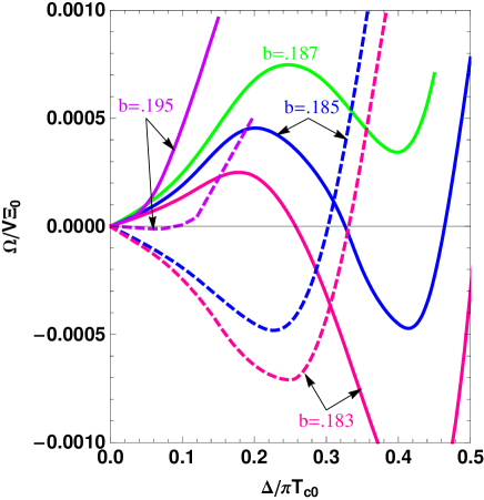
Figure 1: (color online) $\Omega$ vs. $\overline{\Delta}_{\max}$ (in units of $\Xi_{0}V$) for a uniform ($\ q=0$ ) SC order parameter (solid curves) and for the corresponding FF modulated order parameter (dashed curves) at various magnetic field values $b$ near the SC transition at temperature $t=0.02$. The selected g-factor is $\overline{g}=1.8$. Note the second-order transition to the FF state at $b\approx 0.195$ and the first-order transition to the uniform SC state at $b\approx 0.185$.

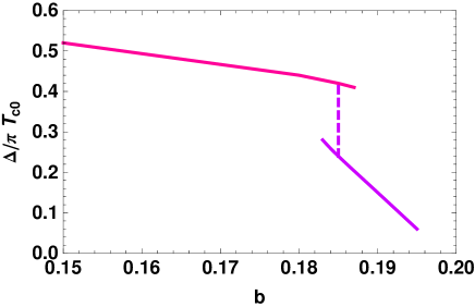
Figure 2: (color online) Field dependence of the self-consistent order-parameter amplitude $\overline{\Delta}_{\max}$ at a temperature $t=0.02$ , well below the tri-critical point ($t_{tric}\approx 0.4$), for $\overline{g}=1.8$.

In the limit of zero spin splitting and in the absence of FF modulation ($g=q=0$) the effective pairing parameter, $X_{\nu}\left(k,k_{z}\right)\equiv\overline{\Delta}_{\max}^{2}\Phi_{\nu}^{+}\Phi_{\nu}^{-}$, is always real and positive. Under these circumstances the general form of $\Omega\left(\overline{\Delta}_{\max}^{2}\right)$ at $H<H_{c20}$, as expressed in Eq.(4), possesses the single minimum structure characterizing the usual GL theory.  For $g\neq 0$ , $X_{\nu}\left(k,k_{z}\right)$ can become complex (a feature that can be ”healed” by the presence of the FF modulation wavenumber $q$ ), so that the general form of $\Omega\left(\overline{\Delta}_{\max}^{2}\right)$ may show a maximum at small $\overline{\Delta}_{\max}^{2}$ which is followed by a minimum at larger $\overline{\Delta}_{\max}^{2}$.  The initial maximum reflects the competition between the increasing spin paramagnetic energy and decreasing SC pair-correlation energy as the number of spin-singlet Cooper-pairs is increased.

Typical results of the calculated TP using Eq.(4) for non-zero spin-splitting are show in Fig.1. As discussed above, the restriction to SC states with $q=0$ , represented in Fig.1 by the solid curves, leads to formation of a maximum at small $\overline{\Delta}_{\max}$ and a local minimum at larger $\overline{\Delta}_{\max}$ by the strong spin splitting effect as the magnetic field is reduced. Upon further field decrease the minimum becomes global and so should drive a first order normal-to-SC phase transition. Allowing for states with $q\neq 0$, however, the unusual feature (i.e. ${Im\ }X_{\nu}\left(k,k_{z}\right)\neq 0$ ) associated with the strong spin splitting effect is ”healed”, and the usual single minimum picture is restored (see the dashed curves in Fig.1). Thus, instead of the ”expected” first-order transition to a uniform SC state one finds a second-order phase transition to a nonuniform (FF) SC state.

However, due to its compensation effect, the FF modulation significantly reduces the equilibrium SC free energy with respect to its uniform counterpart (compare the dashed curves to the corresponding solid ones). As a result, the field range of stability of the modulated phase is quite small. Thus, by slightly reducing the field below the second order normal-to-SC transition the $q=0$ state becomes energetically more favorable and the system transforms from the nonuniform to a uniform SC state via a first-order phase transition. One should note that the second order perturbation theory with $\Omega/V\Xi_{0}=\alpha\left(q\right)\overline{\Delta}_{\max}^{2}+\frac{1}{2}\beta\left(q\right)\overline{\Delta}_{\max}^{4}$, is quantitatively correct only for small values of the order parameter,namely for $\overline{\Delta}_{\max}\lesssim.1$, and, therefore, cannot be applied to the first order transition.

Fig.2 shows the calculated self-consistent $\overline{\Delta}_{\max}^{2}$ (which is optimized with respect to $q$ ) as a function of magnetic field at a temperature well below the tri-critical temperature and for characteristic parameters corresponding to URu₂Si₂.  The initial build-up of the SC order parameter in a narrow region following the second-order phase transition and the pronounced jump at the next (first order) transition are apparent. The overall width of the two-stage transition ($\Delta b/b\approx 0.06$ ) is in good agreement with the width of the sharp structure observed experimentally in the thermal transport measurements Kasahara07 .

Fig.3 exhibits the result of a detailed fitting procedure of our calculation to the experimental data of the dHvA oscillations observed by Ohkuni et. al Ohkuni99 in the mixed state of URu₂Si₂.  The data shows a very sharp reduction in the amplitude of the dHvA oscillation, $A_{SC}$ , just below $H=2.78$ T , similar to the step-like structure observed in the thermal conductivity measurements Kasahara07 . For fitting the measured relative signal, $A_{SC}/A_{n}$ ( $A_{n}$ being the theoretical dHvA amplitude as extrapolated from the normal state) in the region above the sharp damping interval, we exploit the fluctuating vortex lattice model described in Refs.RMP01 ,Maniv06 and write: $\ln\left(A_{SC}/A_{n}\right)=-\frac{\pi^{3/2}}{\hbar\omega_{c}\sqrt{E_{F}\hbar\omega_{c}}}\left\langle\Delta^{2}\right\rangle$ , where $\left\langle\Delta^{2}\right\rangle$ is the mean-square order parameter for the modulated FF state in the vicinity of the second-order phase transition,i.e.: $\left\langle\Delta^{2}\right\rangle=\frac{a_{x}}{2\sqrt{2\pi}}\Delta_{\max}^{2}\left(1+\sqrt{1+\nu_{\kappa}^{2}/x^{2}}\right)$, with $x=\frac{a_{x}}{\sqrt{2\pi}}\sqrt{\frac{\beta\Xi_{0}V_{0}}{2k_{B}T}}\overline{\Delta}_{\max}^{2}$, and $\nu_{\kappa}=0.51$ for a 3D system (see Ref.Maniv06 ). Here $\beta$ is the coefficient of the quartic term obtained in the expansion of $\frac{\Omega}{V\Xi_{0}}$ in $\overline{\Delta}_{\max}^{2}$ near the SC transition, and $V_{0}=\pi^{2}a_{H_{c2}}^{2}/k_{F}$. The selected value of $E_{F}$ has been determined from the experimentally observed, dominant dHvA frequency, $F_{\alpha}\approx 10^{3}$ T, corresponding to the nearly spherical band 17-hole Fermi surface reported in Ref.Ohkuni99 .

The values of $\overline{\Delta}_{\max}^{2}$ at $H<H_{c2}$ were determined in this calculation by minimizing the TP $\Omega$ with respect to both $\overline{\Delta}_{\max}^{2}$ and $\overline{q}$ (see Fig.2), whereas at $H>H_{c2}$ they were obtained by the analytical continuation of the perturbative mean field expression, $\overline{\Delta}_{\max}^{2}=-\alpha/\beta$ into the region $-\alpha/\beta<0$, where $\alpha$ and $\beta$ are the quadratic and quartic coefficients respectively in the perturbation expansion of $\Omega\left(\overline{\Delta}_{\max}^{2}\right)$. The optimal value of $\overline{q}$ in this region was selected by minimizing with respect to $\overline{q}$ the free energy obtained from the functional integral of $e^{-\Omega\left(\overline{\Delta}_{\max}^{2}\right)/k_{B}T}$ over $\overline{\Delta}_{\max}^{2}$, which amounts in the Gaussian approximation to minimizing $\alpha$ with respect to $\overline{q}$.  In the fitting procedure we have exploited the interpolation formula  $\left\langle\Delta^{2}\right\rangle=\frac{1}{2}D_{0}^{2}\left(1-H/H_{c2}\right)+\sqrt{\alpha_{I}^{2}+\frac{1}{4}D_{0}^{4}\left(1-H/H_{c2}\right)^{2}}$Maniv06 with the best fitting adjustable parameters $D_{0}=4.2\ K$, $H_{c2}=2.76\ T$ , and $\alpha_{I}=.06\ K$ (see Fig.3). The resulting value of the order parameter is in a reasonably good agreement with the zero-field gap parameter $\Delta_{BCS}=1.76k_{B}T_{c0}=2.5\ K$ obtained within BCS theory with the experimental value of $T_{c0}\$($=1.4\ K$ ).

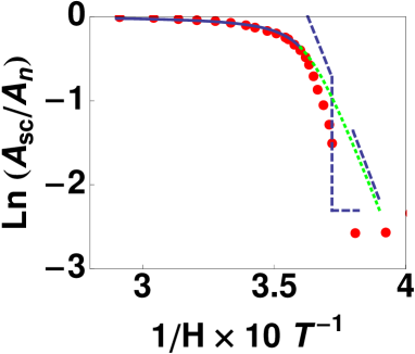
Figure 3: (color online) Logarithm of the dHvA amplitude ratio $A_{SC}/A_{n}$ reported in Ref.Ohkuni99 (full circles) and the values of $-\chi\left\langle\Delta^{2}\right\rangle,\chi=\frac{\pi^{3/2}}{\hbar\omega_{c}\sqrt{E_{F}\hbar\omega_{c}}}$ as obtained from our calculation near the second order phase transition (solid line), as functions of $1/H$. The dashed broken straight line is our mean-field result for $-\chi\Delta_{\max}^{2}$ around the first-order transition. The doted line represents the extrapolation of $-\chi\left\langle\Delta^{2}\right\rangle$ for the modulated FF state to the low-field regime.

Using the resulting parameters and the field dependent $\overline{\Delta}_{\max}^{2}$ shown in Fig.2, we have calculated the jump of $\ln\left(A_{SC}/A_{n}\right)$ at the first order phase transition within our nonperturbative mean field theory. The agreement with the experimental data is good, keeping in mind that thermal fluctuations and inhomogeneous broadening could be responsible for the observed smearing of the theoretical discontinuous transition. Nevertheless, the sharp downward deviation of the experimental data in Fig.3 from the extrapolation of the calculated $-\chi\left\langle\Delta^{2}\right\rangle$ for the modulated FF state to the low-field regime provides a strong evidence for the two-stage nature of the SC transition. It should be stressed that the relative size of the jump in $\Delta_{\max}^{2}$ obtained in our calculation is nearly independent of the various parameters involved, provided the temperature $t$ is well below the tri-critical point $t_{tric}$.

In conclusion, using a non-perturbative approach, we have firmly established our early conjecture concerning the SC transition in a 3D strongly type-II superconductor in the paramagnetic limit, and show that the dHvA effect observed in the mixed SC state of URu₂Si₂Ohkuni99 provides a clear experimental evidence for the double-stage nature of this transition, which is smeared by significant SC fluctuations effect. This finding is consistent with the interpretation of a first-order phase transition given in Ref.Kasahara07 to the step-like structure observed in the thermal transport data of this material. We note that the unusual sign of the observed jump in the thermal conductivity, which could be due to some peculiar quasi-particle scattering mechanism AdachiSigrist08 , is irrelevant to our main argument, which associates this jump, irrespective of its direction, to the jump of the SC order parameter at the predicted first-order transition.

We thank J. Wosnitza, B. Bergk and Y. Kasahara for valuable discussions. This research was supported by the Israel Science Foundation founded by the Academy of Sciences and Humanities, by Posnansky Research fund in superconductivity, and by EuroMagNET under the EU contract RII3-CT-2004-506239.

References

(1) G. Sarma, J. Phys. Chem. Solids 24 , 1029 (1963).
(2) K. Maki and T. Tsuneto, Prog. Theor. Phys. 31, 945
(1964).
(3) T. Maniv and V. Zhuravlev, Phys. Rev. B 77 , 134511
(2008).
(4) P. Fulde and R.A. Ferrell, Phys. Rev. 135, A550,
(1964).
(6) H. Ohkuni, Y. Inada, Y. Tokiwa, K. Sakurai, R. Settai, T.
Honma, Y. Haga, E. Yamamoto. Y. Onuki, H. Yamagami, S. Takahashi and T.
Yanagisawa, Phil. Mag. B 79, 1045 (1999).
(7) Y. Kasahara et al., Phys. Rev. Lett. 99,
116402 (2007).
(8) V. Zhuravlev, T. Maniv, I. D. Vagner, and P. Wyder, Phys.
Rev. B 56 , 14693 (1997).
(9) T. Maniv, V. Zhuravlev, I. D. Vagner, and P. Wyder, Rev.
Mod. Phys.,73, 867.
(10) T. Maniv, V. Zhuravlev, J. Wosnitza, O. Ignatchik, B.
Bergk, and P.C. Canfield, Phys. Rev. B 73, 134521-7 (2006).
(11) Hiroto Adachi and M. Sigrist, arXiv
[cond-mat.super-con]: 0710.3110