Decoding Network Codes by Message Passing
Abstract
In this paper, we show how to construct a factor graph from a network code. This provides a systematic framework for decoding using message passing algorithms. The proposed message passing decoder exploits knowledge of the underlying communications network topology to simplify decoding. For uniquely decodeable linear network codes on networks with error-free links, only the message supports (rather than the message values themselves) are required to be passed. This proposed simplified support message algorithm is an instance of the sum-product algorithm. Our message-passing framework provides a basis for the design of network codes and control of network topology with a view toward quantifiable complexity reduction in the sink terminals.
I Introduction
Network coding [1] is a generalization of routing where intermediate nodes forward coded combinations of received packets (rather than simply switching). This approach yields many advantages, which by now are well documented in the literature [2, 3, 4]. For the single session multicast problem, it is well known that linear network codes are optimal and can achieve the fundamental limit characterized by the min-cut bound [5]. Linear network codes are strongly motivated by practical considerations, namely the implementation of encoders and decoders. Encoders compute linear combinations of received packets, and decoding may be achieved by solving a system of linear equations (since the sink terminals receive a linear transformation of the source data). The standard approach for decoding is Gaussian elimination followed by back-substitution. The resulting decoding complexity is cubic in the size of the linear system, and is essentially independent of the underlying topology.
However, the topology of the underlying communications network has a direct impact on the structure of the linear system that requires solution. This admits the possibility of faster decoding algorithms which exploit such structure. As one example, it is well known that band-diagonal systems may be solved with complexity that scales quadratically in the bandwidth [6]. Similarly, there are many low-complexity iterative solvers for large sparse linear systems [7] (although it should be noted that such iterative methods are usually confined to operating over real or complex fields). This paper is motivated by the possibility of faster decoding algorithms, which exploit knowledge of the network topology.
Let a directed acyclic graph, model a communications network with nodes and directed links . We assume that there are sources, generating source symbols at nodes . Let be the (network coded) symbol transmitted along link .
For any link , define
To simplify notation, we will use the following conventions: (1) for any undirected graph is the set of neighboring nodes of , (2) for any function , we denote its support by and (3) for any function and for each , we denote the set .
We are particularly interested in vector linear network codes over a finite field , where for and . Encoding is according to
where the are the local encoding coefficients and it is assumed that are independent and uniformly distributed over .
The following example motivates careful exploitation of network structure by the decoding algorithm.
Example 1
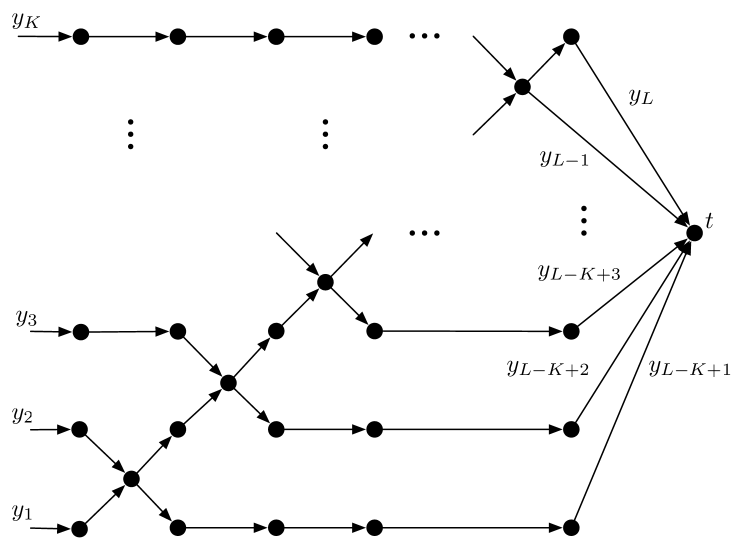
Consider the network in Figure 1with sources . The receiver aims to reconstruct all source symbols. Clearly, decoding can be done by directly solving
where the matrix depends on the choice of local encoding coefficients. Direct solution involves inversion of the matrix , which is . On the other hand, due to the network topology, it is easy to show that where each matrix has at most non-zero entries, located on the diagonals and at the and entries. Inversion of the is very simple (essentially having the same complexity as inverting a matrix). Therefore, we can solve the system of linear equations by computing
| (9) |
Thus for the particular network topology of Figure 1, decoding may actually be achieved in .
The obvious fundamental question is how to reduce decoding complexity, exploiting the topology of an arbitrary network. We propose to use network topology to construct a factor graph for the network code, resulting in a simple message-passing decoding algorithm. Despite the simplicity of this idea, to the best of our knowledge, this paper is the first systematic development of these methods for linear network codes. Iterative decoding in a network coding setting has been briefly considered in [8], however this work was for a specific network topology, and did not develop the idea more generally. Iterative decoding has also been considered in [9] in which the decoding structure was imposed by a Low Density Parity Check degree distribution instead of the topology of the network.
Section II provides the necessary background on factor graphs, and introduces a new “support passing” algorithm. Roughly speaking, this is the sum-product algorithm for scenarios where we don’t care about the “probabilities” themselves, only whether they are non-zero. In Section III we describe how to construct factor graphs from network codes, and show that the messages utilized by the support-passing algorithm are cosets of linear subspaces. Section IV describes how to ensure convergence to the desired solution via clustering operations.
II Factor graphs and message passing
Factor graphs [10] are a graphical representation of the factorization of a global function into a product of local functions. Factor graphs (and related graphical structures such as Bayesian networks and Tanner graphs) and the attendant message passing algorithms for marginalization of the global function have found widespread application [11]. In particular, these methods are a key ingredient in modern coding schemes such as low-density parity check codes [12].
Definition 1 (Factor graph)
Consider a global function that factors into a product of local functions
where is a subset of . A factor graph for is a bipartite graph with variable nodes , factor nodes and edges
Direct brute-force computation of the marginals of a global function is computationally expensive. However if the global function factors in a simple manner, computing marginals can be simplified using the well-known sum-product algorithm [10], briefly reviewed below. Recall that the sum and product operations involved are those of the relevant semi-ring [13].
Definition 2 (Sum-Product Algorithm)
At step , messages are sent from variable nodes to a factor nodes , and messages are sent from factor nodes to a variable nodes . The message updating rules are
| (10) | ||||
| (11) |
where
A well-known fundamental result (see e.g. [10]) regarding the optimality of the sum-product algorithm is restated as follows.
Theorem 1 (Factor tree)
If the factor graph is a tree, then after a finite number of updates, all messages will remain unchanged. Furthermore, for any ,
| (12) |
Theorem 1 shows that when the underlying factor graph is a tree, the sum-product algorithm yields the desired marginals by (12). If the underlying graph is not a tree, then the sum-product algorithm may not converge, and if it does converge, it may converge to an incorrect solution.
As we shall see in Section III, there are meaningful scenarios where we are not interested in the value of the marginals, but rather their support. In such cases, we can simplify the sum-product algorithm.
Theorem 2 (Support passing algorithm)
Assume all local functions are nonnegative. Let and be messages being passed by the sum-product algorithm. Then
| (13) | ||||
| (14) |
and
Proof:
By direct verification. ∎
According to Theorem 2, if only the supports of the marginals are required, then one can simplify the sum-product algorithm by passing only the supports of the messages. Furthermore, the message update rules are given by (13) and (14).
Theorem 3 (Convergence of the support passing algorithm)
Let be the global function and assume the support passing algorithm is used. Initialize for all variable node , where is the alphabet of variable . Then
-
1.
and for all . Hence, after a finite number of iterations, supports of message will remain unchanged;
-
2.
is a subset of and .
Theorem 3 guarantees convergence of the support passing algorithm, even for graphs with cycles. If the factor graph is a tree, the algorithm converges to the support of the marginals. However, if the factor graph contains cycles, it still converges, but to a limit that contains the support of the marginals. Thus the presence of cycles can cause convergence to an undesired solution (although it will “contain” the desired solution).
III Factor Graphs for Network Codes
Let be the symbol generated by the source and be the symbol transmitted on link . For each link , the node receives symbols generated from the sources or transmitted from its neighboring nodes. Considering stochastic encoding, the symbol transmitted on link , namely , is randomly selected according to a conditional distribution . Deterministic codes are obtained via degenerate . Note that this set-up also permits modeling of noisy links (incorporating random errors into the ).
The probability distribution of is
| (15) |
Consider a receiver which observes incoming symbols as for . Then it is straightforward to prove that
| (16) |
With error-free links and a uniquely decodeable code (linear or non-linear), it can easily be shown that decoding is equivalent to finding the support of the marginal of (16). In more general settings, it may be desired to compute the marginal posterior probabilities of the source variables.
In the following, we will provide a mechanical approach to represent the global function (16) with a factor graph. The method works for any network codes. However, as we shall show in the next example, the obtained factor graph may not be the simplest possible.
Definition 3 (Network Code Factor Graph)
Given the network code defined by stochastic local encoding functions , define a factor graph with variable nodes and factor nodes . Each factor node is associated with the local function , and is connected to variable nodes and where . Factor node is associated with the local function , and is connected only to the variable node .
The topology of the above factor graph depends only on the network topology but not the particular codes being used. As a result, the obtained factor graph may not be in its simplest possible form in general. For example, if some local functions can be further factorized into a simpler form, one may be able to further simplify the factor graph. Furthermore, in the context of network coding, only the variables generated by sources are of interest. In that case, it may be possible to prune the factor graph without affecting the decoding process.
Example 2
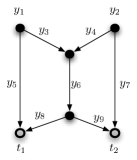
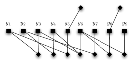
Consider the network shown in Figure 2(a). The symbols generated by the source are and . The receiver can observe symbols and . The factor graph for this code (with respect to the given receiver) is depicted in Figure 2(b).
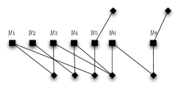
Depending on the specific choices of encoding functions, this factor graph may be simplified. Suppose is a function of . Then one can simplify the factor graph by removing the link between the factor node and the variable node .


.
Let us now consider the special, but important case of deterministic linear network codes. All for are independent and uniformly distributed over and for each link ,
where the local encoding kernel coefficients are fixed and known. Hence,
| (17) | ||||
| (18) |
Theorem 4 (Deterministic linear network codes)
Assume that the support passing algorithm is used. Suppose that is the actual symbol being transmitted or generated. Then
-
1.
and are constant over their supports. Therefore, the support passing algorithm and the sum-product algorithm are equivalent in this case;
-
2.
is a coset of the form where is a vector subspace;
-
3.
Similarly, is also a coset of the form where is also a vector subspace.
Furthermore,
| (19) |
and
| (20) |
where is defined as the minimal subspace containing for all .
Theorem 4, shows that when deterministic linear codes are used, the support passing algorithm can be implemented by “updating” subspaces according to (19) and (20). In the case that the underlying factor graph is acyclic and the network code is uniquely decodeable (i.e. invertible global linear transform), this subspace update algorithm is guaranteed to converge to the correct solution.
Example 3
Consider a butterfly network in Figure 3(a). The sources are and , and the sinks are denoted by open circles. A factor graph for the butterfly network is given in Figure 3(a). Note that, although the butterfly network itself has an undirected cycle, the corresponding factor graph, depicted in Figure 3(b), is cycle-free. Therefore, message passing and support-passing algorithms are exact.
IV Dealing with Cycles
In the previous section, we proposed a simplified sum-product algorithm which passes only the supports of messages. It was proved that the algorithm always converges, and that is equivalent to the sum-product algorithm in the case of deterministic linear network codes. As a result, when the underlying factor graph is a tree, the proposed support-passing algorithm ensures that the support of marginals can be found.
Unfortunately, when the factor graph has cycles, the sum-product algorithm does not always converge. Although support-passing algorithm converges, it may not converge to the supports of the desired marginals.
To avoid cycles, one may transform a factor graph with cycles into one with no cycle. For example, one common transformation technique is clustering [10] as demonstrated in the following example.
Example 4
Consider the network depicted in Figure 4(a), which is a simplified version of the network shown in Figure 1. From the network, we can construct a factor graph in Figure 4(b) according to Definition 3. By clustering function nodes together, we can transform the factor graph into a cycle free one as shown in Figure 4(c). In fact, running the sum-product algorithm over the cycle free factor graph is essentially equivalent to decoding by (9).
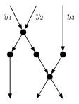
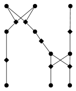
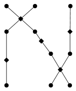
Recall that every link is associated with a factor node. As a general rule, the first step of clustering is to cluster those factor nodes associated with links originating from the same node.
V Conclusion
Decoding of network codes is traditionally achieved by solving a system of linear equations. Using this approach, the decoding complexity of the network is essentially independent of the underlying topology. This paper shows that if we exploit our knowledge of the topology, a more efficient decoding algorithm may be obtained. In some extreme examples, we showed that the reduction in decoding complexity can be huge. This paper prompts a new direction in network code design: how to choose a network subgraph such that the resulting network code admits an efficient decoding algorithm.
As the first step towards the goal, we propose the use of message passing algorithm as a decoding strategy. For a given network code, we give algorithms to construct a factor graph on which message passing algorithms (such as the sum-product algorithm) are performed. We proved that when network links are noiseless, the support passing algorithm (a simplified version of the sum-product algorithm) suffices. We showed that the support-passing algorithm is exact when the underlying factor graph is acyclic and always converges to a limit which contains the desired solutions, even when the factor graph is cyclic. Finally, we discussed the use of some graph augmentation techniques to transform a cyclic factor graph to an acyclic one so that the support passing algorithm is exact.
References
- [1] R. Ahlswede, N. Cai, S.-Y. R. Li, and R. W. Yeung, “Network information flow,” IEEE Trans. Inform. Theory, vol. 46, pp. 1204–1216, July 2000.
- [2] R. W. Yeung, S.-Y. Li, N. Cai, and Z. Zhang, Network Coding Theory. now Publishers, 2006.
- [3] C. Fragouli and E. Soljanin, Network Coding Applications. now Publishers, 2008.
- [4] T. Ho and D. S. Lun, Network Coding: An Introduction. Cambridge University Press, 2008.
- [5] S.-Y. R. Li, R. Yeung, and N. Cai, “Linear network coding,” IEEE Trans. Inform. Theory, vol. 49, pp. 371–381, Feb. 2003.
- [6] G. Golub and C. V. Loan, Matrix Computations. The John Hopkins University Press, 3 ed., 1996.
- [7] O. Axelsson, Iterative Solution Methods. Cambridge University Press, 1994.
- [8] S. Yang and R. Koetter, “Network coding over a noisy relay: a belief propagation approach,” in IEEE Int. Symp. Inform. Theory, 2007.
- [9] A. Montanari and R. Urbanke, “Coding for network coding,” 2007.
- [10] F. R. Kschischang, B. J. Frey, and H.-A. Loeliger, “Factor graphs and the sum-product algorithm,” IEEE Trans. Inform. Theory, vol. 47, no. 2, 2001.
- [11] B. J. Frey, Graphical Models for Machine Learning and Digital Communication. MIT Press, 1998.
- [12] T. Richardson and R. Urbanke, Modern Coding Theory. Cambridge University Press, 2008.
- [13] S. M. Aji and R. J. McEliece, “The generalized distributive law,” IEEE Trans. Inform. Theory, vol. 46, no. 2, pp. 325–343, 2000.