Enhancement of cargo processivity by cooperating molecular motors

Abstract

Cellular cargo can be bound to cytoskeletal filaments by one or multiple active or passive molecular motors. Recent experiments have shown that the presence of auxiliary, nondriving motors, results in an enhanced processivity of the cargo, compared to the case of a single active motor alone. We model the observed cooperative transport process using a stochastic model that describes the dynamics of two molecular motors, an active one that moves cargo unidirectionally along a filament track and a passive one that acts as a tether. Analytical expressions obtained from our analysis are fit to experimental data to estimate the microscopic kinetic parameters of our model. Our analysis reveals two qualitatively distinct processivity-enhancing mechanisms: the passive tether can decrease the typical detachment rate of the active motor from the filament track or it can increase the corresponding reattachment rate. Our estimates unambiguously show that in the case of microtubular transport, a higher average run length arises mainly from the ability of the passive motor to keep the cargo close to the filament, enhancing the reattachment rate of an active kinesin motor that has recently detached. Instead, for myosin-driven transport along actin, the passive motor tightly tethers the cargo to the filament, suppressing the detachment rate of the active myosin.

I Introduction

To carry out its functions, a living cell requires the precise spatiotemporal organization of many macromolecules. Trafficking of molecules within the cytoplasm can be mediated by distinct processes including diffusion, polymerization, and active transport Vale03 . A variety of transport mechanisms may arise from the physical properties of the diverse cargoes being transported. For example, in the case of large cargoes, such as organelles, mRNA or virus particles, diffusion may not be sufficiently fast nor be spatially controlled. These cargoes are often transported by motor proteins that processively move to and from the nucleus along specific cytoskeletal filaments Mallik06 .

The cytoskeleton is typically composed of three types of filaments: microfilaments (e.g. actin), microtubules (e.g. tubulin $\alpha$ and $\beta$), and intermediate filaments (e.g. lamins) Lodish05 . Molecular motors most often associate with and process cargo along actin and microtubules Gross07review . These two filament types are structurally very different from each other. Microtubules (MT) are thicker (25nm diameter) and have a specific radial orientation with respect to the cell nucleus. Actin filaments are more randomly distributed near the periphery of the cell, and are less thick (8nm diameter) than MTs Mallik06 ; Lodish05 . Moreover, filaments are directional. The ends of a microtubule are structurally different and labelled “positive” or “negative,” while the ends of actin filaments are “pointed” or “barbed.” Accordingly, there are different types of motor proteins associated with not only different filament types, but with the direction of transport along these filaments. The MT-specific motor proteins are kinesins (e.g., kinesin I, II) that can move along MTs away from the nucleus on the positive direction, and dyneins that move in the opposite direction towards the negative end of a microtubule Welte04 . Various forms of the actin-specific motor myosin transport cargo toward the barbed (e.g. myoV) or pointed (e.g. myoVI) ends Metha99 ; Gross07 . Since each motor is highly selective, and cargoes need to be moved on both directions of each filament, there are other proteins/cofactors that facilitate molecular transport by associating with specific motors and filaments. For example, dynactin is a cofactor of dynein that enhances both the processivity of dynein and its affinity to certain cargoes Welte04 .

Single molecule imaging methods have been pivotal in the experimental study of molecular motor dynamics Block90 ; Visscher99 . Such advanced techniques have allowed researchers to dissect various aspects of molecular motor mediated transport Shiroguchi07 ; Rief00 ; Carter05 ; Svoboda94 ; Kawaguchi00 ; Clemen05 . The identification of motor proteins, their structure and properties have also led to several theoretical studies Fisher99 ; Kolomeisky03 ; Skau06 ; Kolomeisky07 that have further improved our understanding of how a single motor protein is able to move a cargo along a cytoskeletal filament.

Since many associated proteins/cofactors affect transport dynamics Gross07review , experimental and theoretical investigations of model systems that include only one motor and the tracks on which they bind do not yield a complete description of molecular motor based transport in vivo. Therefore, other recent studies have focused on how cooperativity among different molecular motors can facilitate cargo transport along straight, branched, and intersecting cytoskeletal filaments Gross07 ; Vilfan08 ; Kunwar08 . In the experiments of Ali et al. Ali07 ; Ali08 the cargoes were fluorescently labeled quantum dots (Qdots) Alivisatos05 simultaneously attached to one kinesin and one myoV motor. While analyzing the dynamics of myoV transport in the presence of both actin and MT filaments, the authors discovered that myoV, besides processing along actin, is also able to associate with, and diffuse along microtubules. In further work Ali08 , the same authors showed that when both myoV and kinesin motors are attached to a single cargo, the processivity of the entire assembly is increased on both MT and actin filaments.

Figure 1: Schematic of movement along a filament track of a cargo (blue circle) with both an active (green) and passive (red) motors attached. Each figure represents one of three possible states the cargo complex can be in before detachment, together with the rate constants that lead the system out of a state. Note that the complex moves processively only if the active motor is attached. Only in state $(0,1)$ can the system diffuse.

In this paper, we develop a stochastic model for the cooperative enhancement of kinesin and myoV as discovered in Ali08 . Related stochastic models, both discrete and continuous have been effectively used to model single motor dynamics Skau06 ; Milescu06 and cooperativity Klumpp05 . When applied to single motors, these stochastic models describe the stepping dynamics of typically two-headed molecular motors (e.g. myoV or kinesin) that walk hand-over-hand along the filament, where the trailing and the leading heads exchange roles at each step. In our analysis, we take a coarser approach by treating the entire kinesin-myoV-cargo complex as a single structure that can exist in four possible states corresponding to different association states of each motor with each filament type. From the model we extract and briefly discuss the expressions for the mean run length and the first passage time before detachment. In the Analysis & Discussion section, we fit the model to the experimental results from Ali07 ; Ali08 . The fitting highlights a qualitative difference between cargo transport on actin and microtubules. We also discuss the dependence upon the initial conditions of the system and perform a sensitivity analysis on the unknown parameters.

II Stochastic Multistate Transport Model

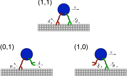
Consider the molecular transport system of a cargo with two motor-proteins attached, one that acts as an active motor (e.g. kinesin on MT) and one that act as a passive motor or tether (e.g. myoV on MT). We denote the state of the engine $\sigma_{a}$ and of the passive tether $\sigma_{p}$ by an ordered pair $\sigma=(\sigma_{a},\sigma_{p})$, where $\sigma_{a,p}=1$ if the active/passive motor is attached to the filament track and where $\sigma_{a,p}=0$ otherwise. Using this notation, state $\sigma=(1,1)$ corresponds to the case where both engine and tether attach cargo to the filament. State $(1,0)$ represents a cargo complex whose engine is attached, but where the tether has detached from the filament (although it remains attached to the cargo). Conversely, $(0,1)$ denotes the case where the engine has detached from the filament, but the tether still holds the cargo on the track. Finally, when both motors have detached from the filament, the complex reaches the $(0,0)$ state. The states of the cargo system are schematically shown in Fig. 1. We only consider states in which, at any given time, at most only one active motor and one passive motor tether can attach a cargo to a filament. This assumption is reasonable because the procedure used in Ali08 for motor attachment predicts that 95$\%$ of the Qdots used as cargo have only one active motor attached. While there are no predictions about the number of tethers attached to the cargo, the relatively small size of the Qdots used in the experiments ($\sim 15$ nm diameter) suggests that simultaneous attachment of an active motor and multiple tethers is highly unlikely.

The cargo complex can move processively along a filament only if the active motor is attached to both cargo and filament. In our notation, this corresponds to states with first index one, e.g. $(1,1)$ or $(1,0)$. In state $(0,1)$, the cargo is either diffusing or immobile, depending on the property of the passive motor. Within this context, we can write the Master equation for the probability density function $P_{\sigma}(x,t)$ that the motor-cargo complex is in state $\sigma$ between position $x$ and $x+\mbox{d}x$ at time $t$:

$${\partial P_{\sigma}(x,t)\over\partial t}+v_{\sigma}{\partial P_{\sigma}(x,t)\over\partial x} = D_{\sigma}{\partial^{2}P_{\sigma}(x,t)\over\partial x^{2}}+\sum_{\sigma^{\prime}}\left[W(\sigma,\sigma^{\prime})P_{\sigma^{\prime}}(x,t)-W(\sigma^{\prime},\sigma)P_{\sigma}(x,t)\right].$$ (1)

Here, $v_{\sigma}$ is the velocity of the cargo in state $\sigma$. This velocity will depend on the specific properties of the motor-protein and on any externally applied forces. For example, as has been well established under many experimental conditions Kawaguchi00 ; Kunwar08 opposing forces applied to motor-driven cargoes linearly decrease their velocity.

Consistent with observations, we set the diffusion constant $D_{\sigma}=0$ in Eq. 1 when an active, driving motor is attached, suppressing random diffusional motion. Conversely, when only a passive tether is attached, the motion of the cargo is Brownian and $D_{\sigma}>0$.

The last term in Eq. 1 represents transitions among binding states $\sigma$. The corresponding rates $W(\sigma,\sigma^{\prime})$ are assumed to be constant and are defined in Table 1. Note that we make the physically reasonable assumption that a cargo complex in state $(1,1)$ cannot have both motors detach simultaneously from the filament track, allowing no transition between state $(1,1)$ and $(0,0)$.

We will analyze the model given by Eq. 1 by defining the probability density vector ${\bf P}(x,t)=(P_{(0,0)},P_{(0,1)},P_{(1,0)},P_{(1,1)})^{T}$. If we assume that the filament track is infinitely long and that the cargo is at position $x=0$ at initial time $t=0$, the initial condition is ${\bf P}(x,t=0)=(0,\alpha,\beta,1-\alpha-\beta)^{T}\delta(x)$, where $\alpha$ is the probability that the cargo complex is initially bound to the filament only by the passive tether, and $\beta$ is the probability that the cargo complex is initially bound only to the active motor. While it is experimentally difficult to quantify $\alpha$ and $\beta$, it is relatively straightforward to determine how our main results for residence times and run lengths depend on the initial conditions. We can therefore establish, a posteriori, the importance of $\alpha,\beta$ in the measured results. Thus, by studying how certain estimated quantities depend on the initial conditions, we can determine the significance and usefulness of experimentally pinpointing the exact values of $\alpha$ and $\beta$.

Table 1: Description of transition rates $W(\sigma,\sigma^{\prime})$ in Eq. 1.

State Transition	Rate	Description
$(1,1)\rightarrow(0,1)$	$d_{\rm{a}}$	Detachment rate of motor from motor-tether complex.
$(1,1)\rightarrow(1,0)$	$d_{\rm{p}}$	Detachment rate of tether from motor-tether complex.
$(0,1)\rightarrow(1,1)$	$k_{\rm{a}}$	Attachment rate of motor to tether only complex.
$(1,0)\rightarrow(1,1)$	$k_{\rm{p}}$	Attachment rate of tether to motor only complex.
$(1,0)\rightarrow(0,0)$	$\mu_{\rm{a}}$	Detachment rate of motor from motor only complex.
$(0,1)\rightarrow(0,0)$	$\mu_{\rm{p}}$	Detachment rate of tether from tether only complex.

The analysis is facilitated by defining the Laplace transform in time $\tilde{{\bf P}}(x,s)=\int_{0}^{\infty}{\bf P}(x,t)e^{-st}\mbox{d}t$, and by taking the dual Laplace-Fourier transform of Eq. 1:

$$s\hat{{\bf P}}(q,s)-\left(\begin{array}[]{c}0\\[13.0pt] \alpha\\[13.0pt] \beta\\[13.0pt] 1-\alpha-\beta\end{array}\right)+\left(\begin{array}[]{cccc}0&0&0&0\\[13.0pt] 0&D_{p}\;q^{2}&0&0\\[13.0pt] 0&0&iqv_{a}&0\\[13.0pt] 0&0&0&iqv_{a}\end{array}\right)\hat{{\bf P}}=\left(\begin{array}[]{cccc}0&\mu_{\rm{p}}&\mu_{\rm{a}}&0\\[13.0pt] 0&-k_{\rm{a}}-\mu_{\rm{p}}&0&d_{\rm{a}}\\[13.0pt] 0&0&-k_{\rm{p}}-\mu_{\rm{a}}&d_{\rm{p}}\\[13.0pt] 0&k_{\rm{a}}&k_{\rm{p}}&-d_{\rm{a}}-d_{\rm{p}}\end{array}\right)\hat{{\bf P}},$$ (2)

where $\hat{{\bf P}}(q,s)=\int_{-\infty}^{\infty}\tilde{{\bf P}}(x,s)e^{-iqx}\mbox{d}x$. In the above equation, and in the remainder of the paper, we use the subscripts $a$, $p$ and $ap$ to indicate the quantities and/or expressions that are characteristic of a transport complex consisting of an active motor only ($a$), a passive motor only ($p$) or both ($ap$). In Eq. 2, we assumed that motion is purely convective when an active motor attaches the cargo to the filament, and therefore set $D_{a}=D_{ap}=0$. As indicated by the experimental data in Ali08 , the passive tether does not noticeably affect the transport velocity of an active motor. Therefore, we also set $v_{ap}=v_{a}$, where $v_{ap}$ is the intrinsic velocity of cargo in the state $(1,1)$. Finally, since the passive motor acting as a simple tether cannot induce drift along a filament track, we set $v_{p}=0$. After imposing these physical constraints, we solve the Master equation to obtain analytical expressions for the mean run length and time. We will use these expressions to compare our model with experimental data from Ali08 .

II.1 Mean Run Lengths

Having more than one motor attached to a cargo complex typically results in an improved transport efficiency. Experiments by Ali et al. Ali08 show significant increases in the processivity of a cargo when it is also attached to a passive motor. Within our model, the measured processivity is equivalent to the mean run length, $\langle X_{ap}\rangle$, of the cargo complex before detachment. To find its expression, we construct the detachment flux density:

$$J_{ap}(x,t)=\mu_{\rm{a}}P_{(1,0)}(x,t)+\mu_{\rm{p}}P_{(0,1)}(x,t).$$ (3)

We can use the properties of the Laplace and Fourier transforms to find a compact expression for $\langle X^{m}_{ap}\rangle$, the $m^{\rm th}$ moment of the run length before detachment:

$$\begin{array}[]{rl}&\langle X_{ap}^{m}\rangle\displaystyle=\int_{0}^{\infty}\left[\int_{0}^{\infty}J_{ap}(x,t)\mbox{d}t\right]x^{m}\mbox{d}x\\[13.0pt] &\displaystyle=\int_{0}^{\infty}x^{m}\left[\mu_{\rm{a}}\tilde{P}_{(1,0)}(x,s=0)+\mu_{\rm{p}}\tilde{P}_{(0,1)}(x,s=0)\right]\mbox{d}x\\[13.0pt] &\displaystyle=\left(i{\partial\over\partial q}\right)^{m}\hat{J}_{ap}(q,s=0)\bigg{|}_{q=0}.\end{array}$$ (4)

Table 2: Typical values of parameters and mathematical quantities for kinesin/myoV cargo transport.

	Mean Value	Biophysical Setup	Ref.
$\langle X_{a}\rangle$	$\left\{\begin{array}[]{c}0.76\;\mu m\\ 1.7\;\mu m\end{array}\right.$	$\begin{array}[]{c}\mbox{myoV on actin}\\ \mbox{ kinesin on MT}\end{array}$	Ali08
$\langle X_{ap}\rangle$	$\left\{\begin{array}[]{c}1.09\;\mu m\\ 3.7\;\mu m\end{array}\right.$	$\begin{array}[]{c}\mbox{myoV-kinesin on actin}\\ \mbox{myoV-kinesin on MT}\end{array}$	Ali08
$v_{a}$	$\left\{\begin{array}[]{c}0.46\;\mu m/s\\ 0.88\;\mu m/s\end{array}\right.$	$\begin{array}[]{c}\mbox{myoV on actin}\\ \mbox{ kinesin on MT}\end{array}$	Ali08
$\mu_{a}$	$\left\{\begin{array}[]{c}0.60\;s^{-1}\\ 0.51\;s^{-1}\end{array}\right.$	$\begin{array}[]{c}\mbox{myoV from actin}\\ \mbox{ kinesin from MT}\end{array}$	Ali08
$k_{a}$	$>0.2\;s^{-1}$	kinesin to MT	Ali08
$\mu_{p}$	$>0.02\;s^{-1}$	myoV from MT	Ali07
$D$	$0.11-0.26\;\mu m^{2}/s$	myoV on MT	Ali07 ; Ali08

By taking $m=1$ we can find the expression for the mean run length of the motor-tether complex before detachment

$$\langle X_{ap}\rangle = v_{a}\frac{\left({d_{\rm{p}}}+{k_{\rm{p}}}+{\mu_{\rm{a}}}-\beta{\mu_{\rm{a}}}\right)\left({k_{\rm{a}}}+{\mu_{\rm{p}}}\right)+{d_{\rm{a}}}\beta{\mu_{\rm{p}}}-\alpha\left[{\mu_{\rm{p}}}\left({k_{\rm{p}}}+{\mu_{\rm{a}}}\right)+{d_{\rm{p}}}{\mu_{\rm{p}}}\right]}{{d_{\rm{a}}}\;{\mu_{\rm{p}}}({k_{\rm{p}}}+{\mu_{\rm{a}}})+{d_{\rm{p}}}\;{\mu_{\rm{a}}}({k_{\rm{a}}}+{\mu_{\rm{p}}})}.$$ (5)

As expected, Eq. 5 is independent of any diffusion of the passive tether since diffusion on average does not contribute to the mean displacement. The mean run length is a monotonically decreasing function of $\alpha$ for all the physically realistic (i.e. positive) values of the model parameters. On the other hand, the dependence of $\langle X_{ap}\rangle$ on $\beta$ will be monotonically increasing (decreasing) if the term ${d_{\rm{a}}}{\mu_{\rm{p}}}-{\mu_{\rm{a}}}\left({k_{\rm{a}}}+{\mu_{\rm{p}}}\right)$ is positive (negative). The processivity of a cargo complex initially in state $(1,0)$ (when $\beta=1$) is greater than that of a cargo beginning in state $(1,1)$ (when $\beta=0$) only when the detachment rate $d_{\rm a}$ of the active motor from the state when both motors are attached is greater than ${\mu_{\rm{a}}}(1+{k_{\rm{a}}}/{\mu_{\rm{p}}})$, where ${\mu_{\rm{a}}}$ is the detachment rate of the active motor by itself.

Establishing the dependency of Eq. 5 upon the remaining parameters does not lead to an easy expression unless we make some simplifications. We can focus on the limit in which all cargo complexes have both motors attached to the track ($\alpha=\beta=0$) at time zero. This is also the underlying assumption used in Ali08 . In this case, we find that the mean run length before detachment reduces to

$$\langle X_{ap}\rangle=\frac{(k_{\rm{p}}+d_{\rm{p}}+\mu_{\rm{a}})(k_{\rm{a}}+\mu_{\rm{p}})v_{a}}{\mu_{\rm{p}}d_{\rm{a}}(k_{\rm{p}}+\mu_{\rm{a}})+\mu_{\rm{a}}d_{\rm{p}}(k_{\rm{a}}+\mu_{\rm{p}})}.$$ (6)

As expected, $\langle X_{ap}\rangle$ is a monotonically increasing function of ${k_{\rm{a}}}$, ${k_{\rm{p}}}$ and $v_{a}$, and a monotonically decreasing function of ${d_{\rm{a}}}$, ${d_{\rm{p}}}$, ${\mu_{\rm{a}}}$ and ${\mu_{\rm{p}}}$.

The probability density flux $J_{a}$ out of the state where the driving motor is attached can be expressed as

$$J_{a}(x,t)=\mu_{\rm{a}}P_{(1,0)}(x,t)+d_{\rm{a}}P_{(1,1)}(x,t).$$ (7)

Since the final two states $(0,\sigma_{p})$ are both absorbing, we must also set $k_{\rm{a}}=0$ in the evaluation of $J_{a}(x,t)$. The expression for the moments of this density flux is analogous to Eq. 4. The mean run length of a cargo complex conditioned on being bound by an active motor is given by

$$\langle X_{a}\rangle = v_{a}\frac{\beta\left({d_{\rm{a}}}-{\mu_{\rm{a}}}\right)+\left({d_{\rm{p}}}+{k_{\rm{p}}}+{\mu_{\rm{a}}}\right)}{{d_{\rm{p}}}{\mu_{\rm{a}}}+{d_{\rm{a}}}\left({k_{\rm{p}}}+{\mu_{\rm{a}}}\right)},$$ (8)

and is a monotonically increasing (decreasing) function of $\beta$ if ${d_{\rm{a}}}>{\mu_{\rm{a}}}$ (${d_{\rm{a}}}<{\mu_{\rm{a}}}$). Similarly, a simple analysis of Eq. 8 reveals that if $\beta=0$ the mean run length $\langle X_{a}\rangle$ in state $(1,\sigma_{p})$ is a monotonically decreasing function of ${k_{\rm{p}}}$ and a monotonically increasing function of ${d_{\rm{p}}}$ if ${d_{\rm{a}}}>{\mu_{\rm{a}}}$. If ${d_{\rm{a}}}<{\mu_{\rm{a}}}$, the mean run length $\langle X_{a}\rangle$ in state $(1,\sigma_{p})$ is a monotonically increasing function of ${k_{\rm{p}}}$ and a monotonically decreasing function of ${d_{\rm{p}}}$. When the detachment rate of the active motor is independent of its state (e.g., ${\mu_{\rm{a}}}={d_{\rm{a}}}$), $\langle X_{a}\rangle=v_{a}/{\mu_{\rm{a}}}$ is independent of the initial conditions and the properties of the tether.

Finally, the mean run length of a cargo bound only by a passive tether (state $(0,1)$) can be found from

$$J_{p}(x,t)=\left({\mu_{\rm{p}}}+{k_{\rm{a}}}\right)P_{(0,1)}(x,t),$$ (9)

and setting the rates into $(0,1)$ from all absorbing states ${d_{\rm{a}}}=\beta=0$, yielding $\langle X_{p}\rangle=0$. This trivial result stems from the drift-free nature ($v_{p}=0$) of the $(0,1)$ state.

Figure 2: A representative trajectory. The processive runs during states $(1,1)$, $(0,1)$ are assumed to have the same velocity independently of the state they are in. The depicted cargo movement is characterized by three processive runs, all with the same slope (e.g. same velocity) and three diffusive events due to the cargo complex being in state $(0,1)$ before ccomplete detachment at ${\bf X}$. The dashed red line represents a straight trajectory that defines an effective velocity of a complete run before detachment.

II.2 First Passage Times

Together with the mean run length, the data in Ali08 include the average velocities for all experimental motor/tether configurations. To use this data for parameter fitting, we derive analytical expressions for the average duration of a run, i.e., the first passage time to the detached state. In order to evaluate the detachment time of the driving motor anywhere along the filament track, we consider the conditional mean first passage time $T_{a}$ out of states $(1,\sigma_{p})$, for which $\alpha=0$, as follows

$$T_{a} = \frac{\int_{0}^{\infty}\mbox{d}t\int_{-\infty}^{\infty}\mbox{d}x\,\,tJ_{a}(x,t)}{\int_{0}^{\infty}\mbox{d}t\int_{-\infty}^{\infty}\mbox{d}x\,\,J_{a}(x,t)}$$ (10)

$$= \left.-\frac{1}{\hat{J}_{a}(q=0,s)}\frac{\partial\hat{J}_{a}(q=0,s)}{\partial s}\right|_{s=0}.$$

Upon using Eq. 10 and ${k_{\rm{a}}}=0$ together with the initial condition ${\bf P}(x,0)=(0,0,\beta,1-\beta)^{T}\delta(x)$ we find

$$T_{a} = \frac{\beta({d_{\rm{a}}}-{\mu_{\rm{a}}})+({d_{\rm{p}}}+{k_{\rm{p}}}+{\mu_{\rm{a}}})}{}$$ (11)

$$= {{d_{\rm{p}}}{\mu_{\rm{a}}}+{d_{\rm{a}}}({k_{\rm{p}}}+{\mu_{\rm{a}}})}.$$

We can use this result in conjunction with the expression for the mean run length from Eq. 8 to obtain an estimate of the velocity $V_{a}$ of the cargo conditioned on it being attached by the active motor:

$$V_{a}=\frac{\langle X_{a}\rangle}{T_{a}}=v_{a}.$$ (12)

Since the passive motor does not affect the motion of the cargo, the velocity when an active motor is attached is independent of the binding and unbinding of the passive tether. This velocity is that within a single processive run. The velocity averaged over a trajectory composed of both processive and diffusive runs will typically be smaller, as discussed below.

We now compute $T_{ap}$, the mean first time to detachment (state $(0,0)$). Using analogous notation, we find

$$T_{ap} = \frac{\int_{0}^{\infty}\mbox{d}t\int_{-\infty}^{\infty}\mbox{d}x\,\,tJ_{ap}(x,t)}{\int_{0}^{\infty}\mbox{d}t\int_{-\infty}^{\infty}\mbox{d}x\,\,J_{ap}(x,t)}$$ (13)

$$= \left.-\frac{1}{\hat{J}_{ap}(q=0,s)}\frac{\partial\hat{J}_{ap}(q=0,s)}{\partial s}\right|_{s=0},$$

from which we obtain

$$T_{ap}=\frac{({d_{\rm{a}}}+{k_{\rm{a}}})({k_{\rm{p}}}+{\mu_{\rm{a}}}-\beta{\mu_{\rm{a}}})+(\beta({d_{\rm{a}}}-{\mu_{\rm{a}}})+(1-\alpha)({k_{\rm{p}}}+{\mu_{\rm{a}}})){\mu_{\rm{p}}}+{d_{\rm{p}}}({k_{\rm{a}}}+\alpha({\mu_{\rm{a}}}-{\mu_{\rm{p}}})+{\mu_{\rm{p}}})}{{d_{\rm{a}}}({k_{\rm{p}}}+{\mu_{\rm{a}}}){\mu_{\rm{p}}}+{d_{\rm{p}}}{\mu_{\rm{a}}}({k_{\rm{a}}}+{\mu_{\rm{p}}})}.$$ (14)

As in section II.1, we can study the dependence of $\langle T_{ap}\rangle$ on the kinetic parameters by considering the $\alpha=\beta=0$ limit:

$$T_{ap}=\frac{{d_{\rm{p}}}({k_{\rm{a}}}+{\mu_{\rm{p}}})+({k_{\rm{p}}}+{\mu_{\rm{a}}})({d_{\rm{a}}}+{k_{\rm{a}}}+{\mu_{\rm{p}}})}{{d_{\rm{a}}}({k_{\rm{p}}}+{\mu_{\rm{a}}}){\mu_{\rm{p}}}+{d_{\rm{p}}}{\mu_{\rm{a}}}({k_{\rm{a}}}+{\mu_{\rm{p}}})}.$$ (15)

This expression is monotonically decreasing with respect to ${\mu_{\rm{a}}}$ and ${\mu_{\rm{p}}}$, and can be used in conjunction with Eq. 6 to obtain an expression for the mean velocity of cargo transport in presence of an active and a passive motor

$$\langle V_{ap}\rangle=\frac{(k_{\rm{p}}+d_{\rm{p}}+\mu_{\rm{a}})(k_{\rm{a}}+\mu_{\rm{p}})v_{a}}{{d_{\rm{p}}}({k_{\rm{a}}}+{\mu_{\rm{p}}})+({k_{\rm{p}}}+{\mu_{\rm{a}}})({d_{\rm{a}}}+{k_{\rm{a}}}+{\mu_{\rm{p}}})}\;\leq\;v_{a}.$$ (16)

This result indicates that although in states $(1,1)$ and $(1,0)$ the cargo drifts with velocity $v_{a}$, the entire run consists of alternating phases of drifting and diffusive states, resulting in an average effective velocity $V_{ap}\leq v_{a}$, with the two velocities being equal only under certain regimes such as for slow active motor dissociation from state $(1,1)$ (e.g. ${d_{\rm{a}}}\ll 1$) or for very fast tether dissociation from state $(0,1)$ (e.g. ${\mu_{\rm{p}}}\gg 1$). From the above expression one can estimate the ratio $\chi$ of convection times to diffusion times as follows

$$\chi = \frac{|V_{ap}-V_{a}|}{v_{a}}=$$ (17)

$$= \frac{{d_{\rm{a}}}({k_{\rm{p}}}+{\mu_{\rm{a}}})}{{d_{\rm{p}}}({k_{\rm{a}}}+{\mu_{\rm{p}}})+({k_{\rm{p}}}+{\mu_{\rm{a}}})({d_{\rm{a}}}+{k_{\rm{a}}}+{\mu_{\rm{p}}})}\;\leq\;1.$$

The above algebraic expressions for the mean length (e.g. Eq. 5) and duration (e.g. Eq. 14) of a run out of the various states constitute our main mathematical results.

Figure 3: Surface plot of the parameter space that satisfies the conditions of Sec. III.A.1 for the mean run length and first passage time. While both ${k_{\rm{p}}}$ and ${d_{\rm{p}}}$ can have values along the positive real line, ${\mu_{\rm{p}}}$ has an upperbound. If ${\mu_{\rm{p}}}>1.25s^{-1}$ there are no physically realistic values of ${k_{\rm{p}}}$ and ${d_{\rm{p}}}$ that satisfy the conditions $\langle X_{ap}\rangle=3.7$ and $T_{ap}=5.0$. For this plot, $v_{a}=0.88\;\mu m$, ${\mu_{\rm{a}}}={d_{\rm{a}}}=0.52\;s^{-1}$, $k_{a}=1.48\;s^{-1}$.

III Analysis & Discussion

Having obtained analytical expressions for the mean run length and duration, we can use experimental data from Ali08 to study parameter assignment within our model. Because the experimental data refer cooperative motor transport along microtubules and actin, we will also divide the analysis into the two corresponding cases.

III.1 Parameter Fitting

In the absence of external forces $v_{a}$ is constant, $v_{p}=0$, and for fixed initial conditions, the model is characterized by 8 parameters. Only for a few of them it is possible to extract estimates from the available literature (see Table 2). However, we can use certain biophysical constraints stemming from Ali08 to reduce the parameter space as much as possible. Throughout this subsection the analysis is performed with $\alpha=\beta=0$.

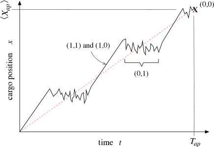
III.A.1 myoV-kinesin transport on MT. Experimental results from Ali08 show that the presence of a passive myoV motor, in addition to an active kinesin motor increases the typical run length of the cargo by two-fold and slightly decreases the velocity by $\sim 15\%$. The same data show that the velocity and mean run length of cargo in state $(1,0)$ and state $(1,1)$ are essentially the same. Fig. 2 is a graphical representation of a possible cargo trajectory showing three processive and three diffusive runs. Since all processive runs are observed to occur with the same velocity, the presence of the passive myosin does not affect the drive of the active kinesin motor. Therefore, both states $(1,0)$ and $(1,1)$ are indistinguishable within each processive run. These observations suggest that we can assume ${d_{\rm{a}}}={\mu_{\rm{a}}}$ in Eq. 1. We used this assumption and the values of $v_{a}$, ${\mu_{\rm{a}}}$ from Table 2 to solve the system consisting of Eq. 6 and Eq. 15 with the constraints $\langle X_{ap}\rangle=3.7\;\mu m$ and $T_{ap}=5.0\;s$ obtained from the experimental results in Ali08 for microtubular transport.

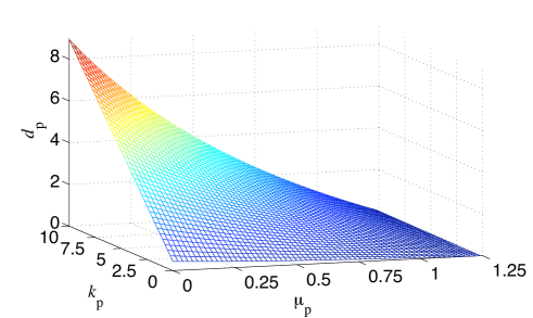
The solution of this system leads to a specific value of $k_{a}=1.48\;s^{-1}$, implying an average diffusion time of $1/{k_{\rm{a}}}=0.68\;s$, consistent with the experimental results in Ali08 . In fact, the average run length of a kinesin-myoV cargo complex on microtubules lasts about 5 seconds and covers twice the distance of a Qdot with only a single kinesin motor attached to it. Therefore, the typical cargo movement due to kinesin/myoV motor consists of two processive steps (needing $\sim 2T_{a}=4.4\;s$, see Ali08 ) and one or two diffusive ones before detachment since we assumed that the cargo is initially in state $(1,1)$. Given such observations, our obtained value of ${k_{\rm{a}}}$ is consistent with the experimental data. More specifically, it suggests that on average there will be only one single diffusive event in between two processive runs.

For the three remaining parameters we find that as long as ${\mu_{\rm{p}}}<1.25s^{-1}$, we can always find $k_{\rm p}$ and ${d_{\rm{p}}}$ that satisfy the physical constraints $\langle X_{ap}\rangle=3.7\;\mu m$ and $T_{ap}=5.0\;s$. These results are shown in Fig. 3. The upper limit for ${\mu_{\rm{p}}}$ implies an average diffusion time of about $0.8$ seconds while in state $(0,1)$ and before detachment. However, the experimental results in Ali07 ; Ali08 show an average diffusion time between $40$ and $60$ seconds in the absence of kinesin. The observed diffusion times are consistent with the value for $k_{a}$ obtained above and suggest that the detachment of the cargo from the microtubule is most likely to happen while the motor is in state $(1,0)$.

Overall, these results suggest that myoV increases the processivity of the cargo complex by keeping kinesin close enough to the track so that its reattach is accelerated. The tethering by myoV occurs without reduction in the intrinsic velocity of kinesin.

Figure 4: Surface plot of the values of ${k_{\rm{p}}}$, ${d_{\rm{p}}}$, and ${d_{\rm{a}}}$ that satisfy the mean run length expression in Eq. 18 when, $v_{a}=0.46\;\mu m$ and ${\mu_{\rm{a}}}=0.60\;s^{-1}$. For ${k_{\rm{p}}}\ll{d_{\rm{p}}}$, ${d_{\rm{a}}}$ tends to the value $0.42s^{-1}$. This value is equivalent to having a cargo complex consisting of only one active and no passive motor.

III.A.2 myoV-kinesin transport on actin. The most striking finding observed using this experimental system is that the processivity is increased by the presence of a passive kinesin tether, but the average velocity remains unchanged, suggesting that the passive tether helps keep the active myoV attached to the filament track without affecting its velocity. In these experiments, one observes longer, uninterrupted processive transport, with rare punctuated moments of diffusive cargo motion. This suggests that the system is predominantly in states $(1,j)$ and that once the active motor detaches, the whole cargo system does too. These observations are consistent with the structural/molecular attributes of this system, since the electrostatic forces between actin and kinesin are too weak to significantly reduce the myosin driven cargo velocity. Moreover, since actin filaments are thin, once myosin detaches, the detachment of kinesin is also fast. But if myosin holds kinesin proximal to the actin filament, the kinesin attachment rate is also fast, since free diffusion is hindered by the tether. Within this context ${d_{\rm{a}}}\neq{\mu_{\rm{a}}}$. We can also assume that ${k_{\rm{a}}}=0$ and that ${\mu_{\rm{p}}}\rightarrow\infty$, leading to the following expressions for the mean run length and first passage time

$$\langle X_{ap}\rangle=\frac{(k_{\rm{p}}+d_{\rm{p}}+\mu_{\rm{a}})v_{a}}{d_{\rm{a}}(k_{\rm{p}}+\mu_{\rm{a}})+d_{\rm{p}}\mu_{\rm{a}}},\langle T_{ap}\rangle=\frac{{d_{\rm{p}}}+{k_{\rm{p}}}+{\mu_{\rm{a}}}}{d_{\rm{a}}(k_{\rm{p}}+\mu_{\rm{a}})+d_{\rm{p}}\mu_{\rm{a}}}.$$ (18)

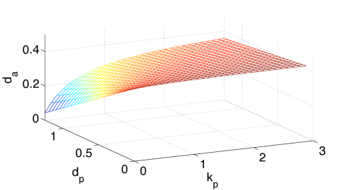
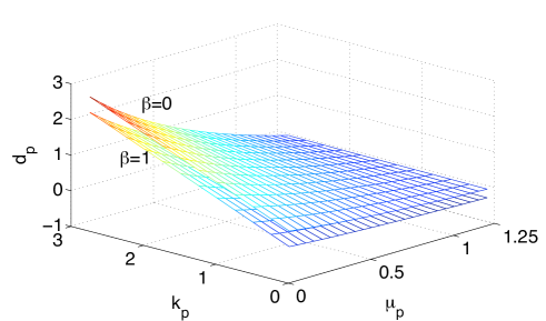
The above expressions are the same as Eq. 8 and Eq. 11 for the particular choice of initial conditions that we have used throughout this section. Moreover, from Eq. 12 we know that the velocity of this system is constantly equal to $v_{a}$. Therefore, the model is able to predict the observed experimental behavior. We can now use $\langle X_{ap}\rangle=1.09\;\mu m$ and $T_{ap}=2.59\;s$ (obtained from Table 1 in Ali08 ) to plot the parameter space that satisfies either one of the expressions in Eq. 18 but not both since they are redundant under the assumption $\langle V_{ap}\rangle=v_{a}$. Using the expression for the mean run length in Eq. 18, we obtain the plot shown in Fig. 4. Here, we see that for ${k_{\rm{p}}}\gg{d_{\rm{p}}}$, ${d_{\rm{a}}}$ reaches a maximum value of $d_{a}=0.42\;s^{-1}$. This quantity is smaller than ${\mu_{\rm{a}}}$, a result that confirms our interpretation that the increase in processivity is due to the tethers ability to prevent detachment of the active motor.

From the properties of actin transport discussed thus far, it seems natural to consider an “effective” detachment rate $\mu_{\rm eff}$ that captures the dynamics of cargo transport in this case:

$$\mu_{\rm eff}=f({\mu_{\rm{a}}},{\mu_{\rm{p}}},{k_{\rm{p}}},{d_{\rm{a}}},{d_{\rm{p}}},v_{a})=\frac{v_{a}}{\langle X_{ap}\rangle}.$$ (19)

From the results in Ali08 , we obtain $\mu_{\rm eff}\approx 0.42\;s^{-1}$. This value is the same as the maximum value obtained above, implying that the overall effect of kinesin is to prevent myoV from detaching from the actin filament, without affecting the intrinsic myoV transport velocity.

Figure 5: Plot of the dependence of ${k_{\rm{p}}}$, ${d_{\rm{p}}}$, and ${\mu_{\rm{p}}}$ on $\beta$ for transport along microtubules. The values of the other parameters are the same as the ones in Fig. 3. Increasing the number of cargo complexes in state $(1,0)$ at time $t=0$ leads to smaller values of tether detachment from state $(1,1)$ for all values of ${k_{\rm{p}}}$ and ${\mu_{\rm{p}}}$.

III.2 Dependence on Initial Conditions

We now investigate how the model fits data as $\alpha$ and $\beta$ in Eq. 2 vary between zero and one. Based on the experimental methodology of Ali08 , we expect both $\alpha$ and $\beta$ to be small. In fact, only Qdots that show a displacement greater than $0.3\;\mu m$ where included in the data, with shorter trajectories discarded, essentially reducing $\alpha$ to zero. The argument for $\beta$ being small also relies upon the experimental methods of Ali et al.. To ensure that each Qdot had at most one active motor and at least a passive one attached to it, they prepared a solution where passive motors were in excess, with molar ratio 16:1 Ali08 .

III.B.1 myoV-kinesin transport on MT. As discussed above, in the case of microtubular transport, we can use the approximation ${d_{\rm{a}}}={\mu_{\rm{a}}}$. Unlike the case with simple initial conditions ($\alpha=\beta=0$), including this constraint in Eqs. 5 and 14 does not yield a simple analytical solution for the mean run length and first passage time before detachment. Therefore, we performed a numerical study of the dependence on the initial conditions and found that for every choice of $\alpha$ and $\beta$ there is only one value of $k_{a}$ that satisfies the experimental results $\langle X_{ap}\rangle=3.7\;\mu m$ and $T_{ap}=5\;s$. In addition, this value depends only on the initial fraction of cargoes in state $(0,1)$ and not on $\beta$. In particular, ${k_{\rm{a}}}$ is a linear function of $\alpha$, with slope $m=1.26\;s^{-1}$, giving us a range of predicted values from ${k_{\rm{a}}}=1.48\;s^{-1}$ (if $\alpha=0$) to ${k_{\rm{a}}}=2.74\;s^{-1}$ (if $\alpha=1$). The increase of predicted ${k_{\rm{a}}}$ with $\alpha$ is not surprising since the higher the probability the systems starts in state $(0,1)$, the faster the kinesin motor will have to bind to the microtubule to satisfy the given time constraint. Conversely, the values of the other free parameters in the model (i.e. 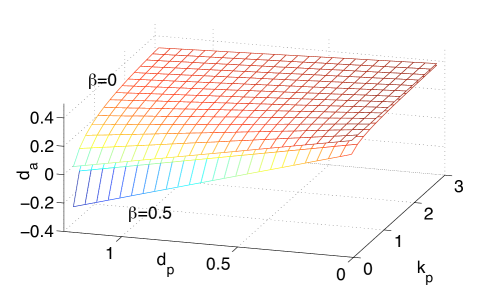${d_{\rm{p}}}$, ${\mu_{\rm{p}}}$, and ${k_{\rm{p}}}$) depend only on the value of $\beta$. This dependence is shown in Fig. 5 for the limit cases $\beta=0$ and $\beta=1$ (in both cases $\alpha=0$). From this plot we notice how an increase in the percentage of cargo complexes in state $(0,1)$ at $t=0$, shifts the parameter surface down along the ${d_{\rm{p}}}$ axis. As a result the parameter space itself in Fig. 5 is reduced, since any combination of parameters resulting in ${d_{\rm{p}}}<0$ is unphysical. From this analysis it seems that all possible initial conditions can explain the experimental data. None of the qualitative observations made in Sec. III.A.1 would change, unless $\alpha>0$. In this case, the average cargo movement would consist of two diffusive steps, one at the beginning of the motion and one at the end of the first processive step.

Figure 6: Plot of the dependence of ${k_{\rm{p}}}$, ${d_{\rm{p}}}$, and ${d_{\rm{a}}}$ on $\beta$ for transport along actin. The values of the other parameters are the same as the ones in Fig. 4. Increasing the number of cargo complexes in state $(1,0)$ at time $t=0$ leads to smaller values of active motor detachment rate from state $(1,1)$. Moreover, some of the values of ${k_{\rm{p}}}$ and ${d_{\rm{p}}}$ lead to negative values of ${d_{\rm{a}}}$ although the limiting behavior for ${k_{\rm{p}}}\ll{d_{\rm{p}}}$ is still the same as for the case $\beta=0$.

III.B.2 myoV-kinesin transport on actin. Using the same assumptions discussed in Section III.A.2, we find the following simplified expression,

$$\langle X_{ap}\rangle=v_{a}\frac{(\beta({d_{\rm{a}}}-{\mu_{\rm{a}}})+(1-\alpha)({k_{\rm{p}}}+{\mu_{\rm{a}}}))+{d_{\rm{p}}}(1-\alpha)}{{d_{\rm{a}}}({k_{\rm{p}}}+{\mu_{\rm{a}}})+{d_{\rm{p}}}+{\mu_{\rm{a}}}},$$ (20)

indicating a mean run length that decreases linearly as $\alpha$ increases. This is physically expected since we assumed ${k_{\rm{a}}}=0$, which implies that diffusional states are not allowed to transition to the processive (1,1) state. How $\langle X_{ap}\rangle$ above scales with $\beta$ depends instead on the difference between ${\mu_{\rm{a}}}$ and ${d_{\rm{a}}}$. The detachment rate of myoV from actin in state $(1,0)$ is about $0.6\;s^{-1}$, and we see from Fig. 4 that this value is never reached (we also verified this result asymptotically). Then, the mean run length of the cargo complex is a decreasing function of the probability of being in state $(1,0)$ at time $t=0$.

The overall effect of a higher value of $\beta$ is to lower the best-fit value of ${d_{\rm{a}}}$ and to reduce the range of physically meaningful parameters, as shown in Fig. 6. Similar to what we mentioned in Section III.B.1, the experimental data can be fit to all possible initial conditions. However, if ${d_{\rm{p}}}$ is too small, the condition for the mean run length from Ali08 cannot be satisfied if $\beta$ is too large. This is reflected by the negative values of the $\beta=0.5$ fit to $d_{\rm a}$ in Fig. 6. These results reinforce the notion that the increased processivity of myoV due to the presence of kinesin depends on the latter’s ability to keep the active motor attached to the track for a longer period of time.

III.3 Sensitivity Analysis

We conclude this section by performing both local and global sensitivity analysis of our model output on the model parameters. Since our goal is to determine the effect of cooperation among different molecular motors on the processivity of cargo transport, we select $\langle X_{ap}\rangle$ (e.g. the mean run length before detachment) as the output of interest.

The simplest local sensitivity analysis evaluates the partial derivatives of the mean run length before detachment with respect to each of the unknown parameters (e.g. $\partial\langle X_{ap}\rangle/\partial{d_{\rm{p}}}$). This determines how sensitive the output is to quantitative changes in each of the kinetic parameters Saltelli05 .

Since local sensitivity analysis is best suited to evaluating output that is linear in the parameters, we will also consider global sensitivity analysis on $\langle X_{ap}\rangle$. This analysis will determine which among the unknown parameters of the model would be most responsible for experimental variation of the output Saltelli04 . This analysis is global in the sense that it spans all of the parameter space. It is model-free, and gives the same result as local sensitivity analysis if the analyzed models are linear Saltelli04 . Let us write $\Omega=\left\{{\mu_{\rm{p}}},{\mu_{\rm{a}}},{d_{\rm{p}}},{d_{\rm{a}}},{k_{\rm{p}}},{k_{\rm{a}}},v_{a}\right\}$ as the input space, and $\Omega_{i}$, $i=1,2,\dots,7$ as $i$-th input in $\Omega$. Then we can define the first-order sensitivity for a fixed input $\Omega_{i}$ as:

$$S_{i}\equiv\frac{V[E(\langle X_{ap}\rangle|\Omega_{i})]}{V[\langle X_{ap}\rangle]},$$ (21)

where $E(\langle X_{ap}\rangle|\Omega_{i})$ is the expected value of the mean run length obtained by uniformly sampling over all other parameters $\Omega_{j\neq i}$, $V[E(\langle X_{ap}\rangle|\Omega_{i})]$ is the variance of the expected mean run length over the parameter $\Omega_{i}$, and $V[\langle X_{ap}\rangle]$ is the unconditional variance of the mean run length. The parameter with highest first order sensitivity index is the one which most influences the variation of the mean run length according to the global sensitivity analysis approach. Global sensitivity analysis can also be used to assess the joint effect of more than one input. We define the second order sensitivity (also known as two-way interaction) as

Figure 7: Local sensitivity analysis of free model parameters in the case of kinesin/myoV cargo transport on microtubules. The parameters for all three of these graphs are $v_{a}=0.88\;\mu m/s$, ${d_{\rm{a}}}={\mu_{\rm{a}}}=0.52\;s^{-1}$, ${k_{\rm{a}}}=1.48\;s^{-1}$, and ${d_{\rm{p}}}=0.5\;s^{-1}$. A: Sensitivity analysis with respect to ${\mu_{\rm{p}}}$, in this case the z-axis represents $\partial\langle X_{ap}\rangle/\partial{\mu_{\rm{p}}}$. B: Sensitivity analysis with respect to ${k_{\rm{p}}}$, in this case the z-axis represents $\partial\langle X_{ap}\rangle/\partial{k_{\rm{p}}}$ C Sensitivity analysis with respect to ${d_{\rm{p}}}$, in this case the z-axis represents $\partial\langle X_{ap}\rangle/\partial{d_{\rm{p}}}$.

$$S_{ij}\equiv\frac{V[E(\langle X_{ap}\rangle|\Omega_{i},\Omega_{j})]}{V[\langle X_{ap}\rangle]},$$ (22)

where $E(\langle X_{ap}\rangle|\Omega_{i},\Omega_{j})$ is the expected value of the mean run length given fixed values of $\Omega_{i}$ and $\Omega_{j}$. Higher order global sensitivity indexes can be analogously defined. We apply local and first and second order global sensitivity analyses to both experimental cases:

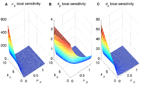
III.C.1 myoV-kinesin transport on MT. Representative results of the local sensitivity analysis for the microtubule case are plotted in Fig. 7. Under certain regimes, ${\mu_{\rm{p}}}$ has the greatest influence on the mean run length before detachment, followed by ${d_{\rm{p}}}$, with ${k_{\rm{p}}}$ as the least influential among the three parameters. To further investigate the results from the local sensitivity analysis, we determine the first and second order global sensitivity indexes for all free parameters. These results are listed in the first row of Table 3. We find that the parameter that is responsible for most of the variation in $\langle X_{ap}\rangle$ is ${d_{\rm{p}}}$.

Both of the analyses predict that ${k_{\rm{p}}}$ has the least influence on the mean run length, but they differ in their ranking of ${\mu_{\rm{p}}}$ and ${d_{\rm{p}}}$. This difference arises from the nonlinearity of Eq. 5 and the intrinsic differences among the two types analyses. Local sensitivity analysis suggests that if we could control the values of the parameters of the system, we would effect the largest changes in $\langle X_{ap}\rangle$ by altering the rate of detachment of myoV while in state $(0,1)$. If experimentally, we are sampling parameter space, global sensitivity analysis predicts that by correctly determining ${d_{\rm{p}}}$ we can achieve the most reduction in the variability of the mean run length.

Table 3: First and second order sensitivity indexes for microtubule and actin cargo transport. To determine these indexes we sampled ${d_{\rm{p}}}$ and ${k_{\rm{p}}}$ uniformly in $[0,20]$ with step $0.05$. For the microtubule case we sample ${\mu_{\rm{p}}}$ in $[0,1.25]$ with step $0.01$. For the actin case we sampled ${d_{\rm{a}}}$ in $[0,0.42]$ with step $0.01$.

	$S_{{k_{\rm{p}}}}$	$S_{{d_{\rm{p}}}}$	$S_{{\mu_{\rm{p}}}}$	$S_{{d_{\rm{a}}}}$	$S_{{k_{\rm{p}}},{\mu_{\rm{p}}}}$	$S_{{k_{\rm{p}}},{d_{\rm{p}}}}$	$S_{{d_{\rm{p}}},{\mu_{\rm{p}}}}$	$S_{{d_{\rm{a}}},{k_{\rm{p}}}}$	$S_{{d_{\rm{a}}},{d_{\rm{p}}}}$
MT	0.06	0.27	0.1	–	0.20	0.35	0.82	–	–
Actin	0.1	0.33	–	0.23	–	0.45	–	0.37	0.81

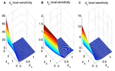
III.C.2 myoV-kinesin transport on actin. The local and global sensitivity analyses also give different results in the case of cargo transport along actin filaments. Three representative plots of the local sensitivity analysis are shown in Fig. 8. These show that the detachment rate of myoV from actin when both motors are attached is the most influential parameter with respect to the mean run length before detachment. However, the first order sensitivity index of ${d_{\rm{a}}}$ is about $1/3$ smaller than the same index for ${d_{\rm{p}}}$ (see Table 3), making the detachment rate of kinesin when in state $(1,1)$ the parameter more responsible for the variance in $\langle X_{ap}\rangle$. In this case, the sensitivity to ${d_{\rm{p}}}$ is consistent with the role of the passive tether in preventing myoV detachment.

Interestingly, both cases (actin and microtubule) have ${d_{\rm{p}}}$ as the free parameter with highest first order sensitivity and ${k_{\rm{p}}}$ as the lowest one. Moreover, if we want to reduce by at least $80\%$ the uncertainty in the determination of the mean run length, we can do so by exactly determining ${d_{\rm{p}}}$ and ${\mu_{\rm{p}}}$ for the microtubule case and ${d_{\rm{p}}}$ and ${d_{\rm{a}}}$ for the actin case (cf. Table 3).

Figure 8: Local sensitivity analysis of free model parameters in the case of myoV/kinesin cargo transport on actin. The parameters for all three of these graphs are $v_{a}=0.46\;\mu m/s$, ${\mu_{\rm{a}}}=0.6\;s^{-1}$, ${k_{\rm{a}}}=0\;s^{-1}$, ${\mu_{\rm{p}}}\ll 1$ and ${d_{\rm{p}}}=0.5\;s^{-1}$. A: Sensitivity analysis with respect to ${\mu_{\rm{p}}}$, in this case the z-axis represents $\partial\langle X_{ap}\rangle/\partial{d_{\rm{a}}}$. B: Sensitivity analysis with respect to ${k_{\rm{p}}}$, in this case the z-axis represents $\partial\langle X_{ap}\rangle/\partial{k_{\rm{p}}}$ C Sensitivity analysis with respect to ${d_{\rm{p}}}$, in this case the z-axis represents $\partial\langle X_{ap}\rangle/\partial{d_{\rm{p}}}$.

IV Summary & Conclusions

We presented a stochastic model that describes the cooperative behavior between two different motors attaching cargoes to a cytoskeletal filament. Of the two motors, one acts as engine, moving the cargo unidirectionally along the filament, while the other acts as a tether. We applied the model to the data from Ali08 , where the authors studied in vitro the cooperative behavior of kinesin and myosin V when moving cargo along microtubules and actin. Experimental visualization indicates significant diffusive dynamics for cargo transport along microtubules in the presence of myosin V, while cargoes transported along actin did not exhibit diffusive dynamics. A consistent interpretation of these observations is that along microtubules, tethers (myosin) predominantly enhances reattachment of the active motor (kinesin). In the case of transport along actin, the kinesin tether acts to prevent detachment of the active myosin motor. This interpretation has been verified within our model. In fact, for the case of microtubule transport we found that the reattachment rate (${k_{\rm{a}}}$) of kinesin to the filament when the tether is attached is three times faster than its corresponding detachment rate. For the case of actin, we found that the detachment rate of myoV when kinesin is attached to the filament is slower than in the absence of the tether for all values in the explored parameter space.

Although most of the modeling effort described in the literature use a very detailed representation of the physical and chemical properties of the molecular motor under investigation, such analysis becomes much more complex when considering multiple cooperating motors. Coarser models such as ours can be straightforwardly extended to incorporate cargo systems with $M$ active motors and $N$ tethers. The state of such cargo complex will be characterized by a $M+N$-tuple, whose first $M$ components have value $1$ or $0$ depending on whether the active motors they represent are attached to the cytoskeletal filament or not. Conversely, the last $N$ components will have value $1$ or $0$ depending on the attachment status of each passive motor. Proceeding as we did in Section II, we can define a Master equation from which mean run lengths and first passage times to full detachment may be determined. As done in the present case, such a model could be used to find the optimal configuration of motor and tethers that fits the available experimental data.

V Acknowledgments

The authors are grateful to Y. Ali, H. Lu, and D. Warshaw for their clarifying comments. This work was supported by grants from the NSF (DMS-0349195, DMS-0719462) and the NIH (K25 AI41935).

References

- (1) R. D. Vale, Cell, 2003, 112, 467.
- (2) R. Mallik and S.P. Gross, Physica A, 2006, 372, 65.
- (3) H. Lodish, A. Berk, P. Matsudaira, C.A. Kaiser, M. Krieger, M.P. Scott, S.L. Zipursky and J. Darnell, W.H. Freeman Co, 2005, 5th Ed.
- (4) S.P. Gross, Curr. Biol., 2007, 17, R277.
- (5) M.A. Welte, Curr. Biol., 2004, 14, R525.
- (6) A.D. Metha, R.S. Rock, M. Rief, J.A. Spudich, M.S. Mooseker and R.E. Cheney, Nature, 1999, 400, 590.
- (7) S.P. Gross, M. Vershinin and G.T. Shubeita, Curr. Biol., 2007, 17, R478.
- (8) S.M. Block, L.S.B. Goldstein and B.J. Schnapp, Nature, 1990, 348, 348.
- (9) K. Visscher, M.J. Schnitzer and S.M. Block, Nature, 1999, 400, 184.
- (10) K. Shiroguchi and K. Kinosita Jr., Science, 2007, 316, 1208.
- (11) M. Rief, R.S. Rock, A.D. Mehta, M.S. Mooseker, R.E. Cheney and J.A. Spudich, Proc. Natl. Acad. Sci. USA, 2000, 97, 9482.
- (12) N.J. Carter and R.A. Cross, Nature, 2005, 435, 308.
- (13) K. Svoboda and S.M. Block, Cell, 1994, 77, 773.
- (14) K. Kawaguchi and S. Ishiwata, Biochem. Biophys. Res. Comm., 2000, 272, 895.
- (15) A.E. Clemen, M. Vilfan, J. Jaud, J. Zhang, M. Barmann and M. Rief, Biophysical J., 2005, 88, 4402.
- (16) M.E. Fisher and A.B. Kolomeisky, Physica A, 1999, 274, 241.
- (17) A.B. Kolomeisky and M.E. Fisher, Biophysical J., 2003, 84, 1642.
- (18) K. I. Skau, R. B. Hoyle and M. S. Turner, Biophysical J., 2006, 91, 2475.
- (19) A.B. Kolomeisky, and M.E. Fisher, Annu. Rev. Phys. Chem., 2007, 58, 675.
- (20) A. Vilfan, Biophysical J., 2008, 94, 3405.
- (21) A. Kunwar, M. Vershinin, J. Xu and S.P. Gross Curr. Biol., 2008, 18, 1.
- (22) M. Y. Ali, E.B. Krementsova, G.G. Kennedy, R. Mahaffy, T.D. Pollard, K. M. Trybus and D. M. Warshaw, Proc. Natl. Acad. Sci. USA, 2007, 104, 4332.
- (23) M. Y. Ali, H. Lu, C. S. Bookwalter, D. M. Warshaw and K. M. Trybus, Proc. Natl. Acad. Sci. USA, 2008, 105, 4691.
- (24) A.P. Alivisatos, W. Gu and C. Larabell, Annu. Rev. Biomed. Eng., 2005, 7, 55.
- (25) L. S. Milescu, A. Yildiz, P. R. Selvin and F. Sachs, Biophysical J., 2006, 91, 3135.
- (26) S. Klumpp and R. Lipowsky, Proc. Natl. Acad. Sci. USA, 2005, 102, 17284.
- (27) A. Saltelli, M. Ratto, S. Tarantola and F. Campolongo, Chem. Rev., 2005, 105, 2811.
- (28) A. Saltelli, S. Tarantola, F. Campolongo and M. Ratto, W.H. Freeman Co, 2005, 5th Ed.