Simulations of Baryon Acoustic Oscillations II: Covariance matrix of the matter power spectrum
Abstract
We use 5000 cosmological -body simulations of Gpc3 box for the concordance CDM model in order to study the sampling variances of nonlinear matter power spectrum. We show that the non-Gaussian errors can be important even on large length scales relevant for baryon acoustic oscillations (BAO). Our findings are (1) the non-Gaussian errors degrade the cumulative signal-to-noise ratios () for the power spectrum amplitude by up to a factor of 2 and 4 for redshifts and , respectively. (2) There is little information on the power spectrum amplitudes in the quasi-nonlinear regime, confirming the previous results. (3) The distribution of power spectrum estimators at BAO scales, among the realizations, is well approximated by a Gaussian distribution with variance that is given by the diagonal covariance component. (4) For the redshift-space power spectrum, the degradation in by non-Gaussian errors is mitigated due to nonlinear redshift distortions. (5) For an actual galaxy survey, the additional shot noise contamination compromises the cosmological information inherent in the galaxy power spectrum, but also mitigates the impact of non-Gaussian errors. The is degraded by up to for a WFMOS-type survey. (6) The finite survey volume causes additional non-Gaussian errors via the correlations of long-wavelength fluctuations with the fluctuations we want to measure, further degrading the values by about 30% even at high redshift .
Subject headings:
cosmology: theory – large-scale structure of universe1. Introduction
Baryon acoustic oscillations (BAO) are imprinted in the distribution of galaxies, of which the characteristic length scale can be used as a standard ruler in the universe (e.g. Eisenstein, Hu & Tegmark 1998; Blake & Glazebrook 2003; Seo & Eisenstein 2003; Matsubara 2004; Guzik, Bernstein & Smith 2007). BAO provides a powerful way of probing the nature of dark energy. Large galaxy surveys such as the Sloan Digital Sky Survey and two degree Field Survey detected the BAO signature and provided constraints on the dark energy equation of state (Cole et al. 2005; Eisenstein et al. 2005; Percival et al. 2007; Okumura et al. 2008; Gaztanaga, Cabre & Hui 2008; Sanchez et al. 2009). Future larger surveys are aimed at measuring the BAO scale more accurately and hence yielding tighter constraints on the nature of dark energy (see e.g. Benitez et al. 2008).
The BAO signature in the galaxy power spectrum is very small, of the order of a few percent modulation in amplitude, and hence measurements of the precise length scale are hampered by a number of effects. For example, nonlinear gravitational evolution, redshift space distortion, galaxy formation processes and the associated scale-dependent bias, all compromise a robust detection. Accurate theoretical models are clearly needed. A number of authors resort to using numerical simulations (Meiksin, White & Peacock 1999; Seo & Eisenstein 2005; Huff et al. 2007; Smith, Scoccimarro & Sheth 2007, 2008; Angulo et al. 2008; Takahashi et al. 2008; Seo et al. 2008; Nishimichi et al. 2008) whereas others use perturbation theory (Crocce & Scoccimarro 2006, 2008; Jeong & Komatsu 2006, 2009; Nishimichi et al. 2007; McDonald 2007; Matarrese & Pietroni 2007, 2008; Pietroni 2008; Matsubara 2008a,b; Taruya & Hiramatsu 2008; Takahashi 2008; Nomura, Yamamoto & Nishimichi 2008; Rassat et al. 2008). It is important to note that one needs accurate estimates not only for the power spectrum but also its covariance (e.g. Scoccimarro, Zaldarriaga & Hui 1999; Meiksin & White 1999; Habib et al. 2007). The covariance describes statistical uncertainties of the power spectrum measurement as well as the band powers at different wavenumbers are correlated with each other. Hence once the well-calibrated covariance is obtained, one can derive unbiased, robust constraints on cosmological parameter from the measured power spectrum (see Ichiki et al. 2008 for such an example to show the importance of the covariance estimation).
The power spectrum covariance matrix has only diagonal elements for the Gaussian density fluctuations (e.g. Feldman, Kaiser & Peacock 1994). The relative error of the power spectrum of a given wavenumber is then simply given by the square root of the number of Fourier modes available from the survey volume. However, at small length scales, non-vanishing off-diagonal parts of the covariance arise due to the mode coupling (Scoccimarro, Zaldarriaga & Hui 1999; Meiksin & White 1999; Smith 2008). This non-Gaussian contribution is described by the trispectrum or the Fourier transform of the 4-point correlation function. Cooray & Hu (2001) used the halo model to estimate the trispectrum contribution and showed that the non-Gaussian errors do degrade the precision of cosmological parameter determination, and therefore cannot be ignored for planned future surveys (see also Takada & Jain 2008; Eifler, Schneider & Hartlap 2008). Also recently, Smith (2008) studied the covariance matrix of the halo power spectrum using numerical simulations. Sefusatti et al. (2006) also studied the power spectrum covariance using PTHalos (Scoccimarro & Sheth 2002).
In this paper, we use an unprecedentedly large number of simulation realizations to estimate the covariance matrix of the matter power spectrum in both real and redshift space. Our sample is more than 2 orders of magnitude larger than those used in the previous works, yielding well-converged estimates on the power spectrum covariance. We compare our simulation results with the analytical estimates based on perturbation theory and halo model. In these comparisons we also include the new effect of non-Gaussian errors that inevitably arise for a finite-volume survey, as first pointed out in Rimes & Hamilton (2005; also see Rimes & Hamilton 2006; Hamilton, Rimes & Scoccimarro 2006; Neyrinck, Szapudi & Rimes 2006; Neyrinck & Szapudi 2007, and Lee & Pen 2008 for the observational implication based on the SDSS data). By using this large number of the realizations, we also study how the power spectrum estimates are distributed in different realizations, i.e. the probability distribution of power spectrum, and then compute the higher-order moments, skewness and kurtosis, to examine the overall impact of power spectra at high sigma ends. Furthermore we estimate the expected signal-to-noise ratio for measuring the power spectrum for a future galaxy survey, taking into account the shot noise contamination and the non-Gaussian errors.
Throughout the present paper, we adopt the standard CDM model with matter density , baryon density , cosmological constant , spectral index , amplitude of fluctuations , and expansion rate at the present time km s-1 Mpc-1, which are consistent with the WMAP 3-year results (Spergel et al. 2007).
2. Numerical Simulations
We use the cosmological simulation code Gadget-2 (Springel, Yoshida & White 2001; Springel 2005). We employ particles in a volume of Mpc on a side. We generate initial conditions of the seed density perturbations at based on the standard Zel’dovich approximation using the matter transfer function calculated by CAMB (Code for Anisotropies in the Microwave Background: Lewis, Challinor & Lasenby 2000). We ran 5000 realizations of Particle Mesh (PM) simulations for the fiducial cosmological model, and use the snapshot outputs at and to study the power spectrum covariances.
To calculate the Fourier transform of the density field, denoted as , we first assign the -body particles onto grids based on the cloud-in-cell method and then perform FFT111FFTW home page: http://www.fftw.org/. We also correct the effect of the cloud-in-cell assignment scheme as with (Hockney & Eastwood 1988; Angulo et al. 2008). The binned power spectrum for a given realization is estimated as
| (1) |
where the summation runs over all the Fourier modes whose length is in the range for a given bin width . Here is the number of modes taken for the summation and is given as for the limit , where is the simulation box size and is the volume given by . The shot noise is not subtracted, since this effect is very small. The ensemble average of the power spectrum estimator is then computed by averaging the estimated spectra over the realizations: .
We have checked that our simulation result for the power spectrum agrees with the higher resolution TreePM result within at /Mpc 222The agreement is achieved in real space. In redshift space, PM simulations somewhat underestimate the power spectrum by at at small length scales (/Mpc). (here the Nyquist wavenumber is Mpc). If the initial redshift is set to be higher, e.g. , the results agree within for /Mpc and for /Mpc for . This is sufficient for our purpose, which is to estimate the impact of nonlinear clustering on the power spectrum covariances at BAO scales.
3. Covariance Matrix
The covariance between the power spectra, and , is estimated from the simulation realizations and can be formally expressed in terms of the Gaussian and non-Gaussian contributions (e.g. Scoccimarro, Zaldarriaga & Hui 1999; Meiksin & White 1999):
| (2) |
where is the trispectrum, and is the Kronecker-type delta function defined such that if within the bin width, otherwise zero. The integration range in the second term is, as in Eq. (1), confined to the Fourier modes lying in the range , and () denotes the integration volume in Fourier space given by for the case of .
The first term of the covariance matrix represents the Gaussian error contribution ensuring that the two power spectra of different wavenumbers are uncorrelated, while the second term gives the non-Gaussian errors that include correlations between power spectra at different ’s arising from nonlinear mode coupling. Both the terms scale with the simulation box volume as . It should be also noted that the non-Gaussian term does not depend on the bin width (because ), so increasing only reduces the Gaussian contribution via the dependence . However, the cumulative signal-to-noise ratio we will study below is independent of the assumed .
We will compare the simulation results with two analytical approaches to estimate the covariance matrix: (1) perturbation theory and (2) halo model. In perturbation theory, following Scoccimarro et al. (1999; also see Neyrinck & Szapudi 2008), the power spectrum and trispectrum are, self-consistently including up to the third order perturbations of , expressed as
| (3) |
where denotes the linear-order spectrum, and and are the one-loop corrections to the nonlinear power spectrum (Makino, Sasaki & Suto 1992; Jain & Bertschinger 1994) and and are the kernels for the second and third order density perturbations (e.g. Bernardeau et al. 2002).
In the halo model, the power spectrum is given by a sum of two terms, the so-called one-halo term and two-halo term (Seljak 2000; Ma & Fry 2000; Peacock & Smith 2000; also see Cooray & Sheth 2002 for a review). Similarly, the trispectrum consists of four terms, from one to four halo terms:
| (4) |
The explicit expressions of each term can be found in Cooray & Hu (2001). In nonlinear regime, i.e. large , the 1-halo term gives dominant contribution to the total power of trispectrum, while the different halos terms become more significant with decreasing and the 4-halo term that includes the PT trispectrum contribution becomes dominant on very small .
To complete the halo model approach, we need suitable models for the three ingredients: the halo mass function (Sheth & Tormen 1999), the halo bias parameters (Mo & White 1996; Mo, Jing & White 1997), and the halo mass density profile (Navarro, Frenk & White 1997), each of which is specified by halo mass and redshift for a given cosmological model. The details of our halo model implementation can be found in Takada & Jain (2003; 2008).
In our previous paper (Takahashi et al. 2008), we found that a finite size simulation causes the growth of large-scale density perturbations to be deviated from the linear theory prediction, and the deviation is well described by the nonlinear mode coupling. We proposed a method to “correct” the deviation in the finite size simulations to obtain the ensemble averaged expectation of power spectrum without running ideal simulations with infinite volume (practically very large volume), as also demonstrated in Nishimichi et al. (2008). In this paper, where we are discussing the power spectrum covariance for some finite survey volume, we do not have to “correct” the deviation in power spectrum of each realization, because the scatters are already included in the covariance formula (the terms with in Eq. [3]).
We use realizations of each output redshift to directly estimate the covariance matrix according to Eq. (2). To be more explicit, denoting the power spectrum of the -th realization as , we can estimate the covariance as
| (5) |
where is the number of realizations, i.e. in our case, and denotes the mean spectrum computed as . As shown in Appendix, the accuracy in estimating the covariances scales with the number of realizations used333More precisely, the accuracy of estimating the covariance is determined by the covariance of the power spectrum covariance that includes up to the 8-point correlation functions (Kayo et al. in preparation).. For example, the relative accuracy of estimating the diagonal covariance elements is found to scale approximately as . Hence, with the aid of 5000 realizations, we can achieve a few %-level accuracies in estimating each elements of the covariance, an improvement by an order of magnitude over previous works.
4. Comparison with Theoretical Models
4.1. Results in Real Space
Fig.1 shows the diagonal elements of the covariance matrix as a function of wavenumbers. The diagonal elements plotted are divided by the Gaussian covariances of linear power spectra at each redshift such that the values become unity in the linear regime limit (). Therefore the deviations from unity arise from the non-linear evolution of and the non-Gaussian covariance contribution. The cross, triangle and circle symbols show the simulation results for redshifts 1 and 0, respectively. Note that we adopt the bin width of Mpc-1 throughout this paper. The deviations from the Gaussian errors become more significant at lower redshifts. For comparison, the solid curves show the analytical predictions obtained when the perturbation theory is employed to estimate the covariances as described around Eq. (3). The perturbation theory fairly well reproduces the simulation results within up to Mpc at and Mpc at and , respectively. However, at lowest redshift , stronger nonlinear effects are seen even on these large length scales corresponding to the BAO scales. The dashed curves show the halo model results which take into account of this nonlinear effect. The halo model fairly well fits the simulation results over the range of wavenumbers studied. At the PT predicts the larger variance than the halo model, because the one-loop power spectrum in the Gaussian term (3) overestimate the power spectrum.
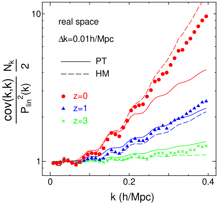
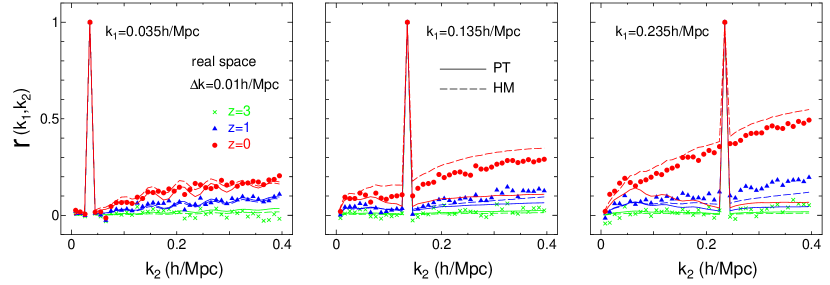
Fig.2 shows the off-diagonal elements of the covariance matrix. For illustrative purpose we study the correlation coefficient matrix defined as
| (6) |
The coefficients are normalized so that for the diagonal components with . For the off-diagonal components implies strong correlation between the two spectra, while corresponds to no correlation. Note again that the matrix elements depend on the bin width: a finer binning, i.e. a smaller , decreases the off-diagonal components. First of all, comparing the three panels of Fig. 2 manifests that the off-diagonal components have greater amplitudes with increasing . The PT fits the data within for Mpc at , for Mpc at and for Mpc at . For the redshift dependence, there is almost no cross-correlations at redshift , while there are increasing cross-correlations at lower redshifts.
The PT results start to underestimate the correlation strengths with increasing and at lower redshifts due to the stronger nonlinearities. Compared to Fig. 1, the PT results are found to be less accurate to describe the off-diagonal components at and 0. The dashed curves are the halo model results, which are in a good agreement with the simulation results, especially at . We found that an inclusion of the 2- and 3-halo terms is important to describe the scale dependences of the off-diagonal correlations. However, the halo model displays a sizable disagreement at some scales, and is not well accurate. Therefore a further refinement of the model predictions based on this kinds of large-scale simulations is needed to accurately model the measurement errors of power spectrum, especially for future high-precision surveys.
4.2. Results in Redshift Space
In this section, we examine the covariance of the redshift-space power spectrum that is a more direct observable in galaxy surveys. The redshift-space power spectrum in each realization is computed as follows. Assuming the distant observer approximation, we first calculate the density perturbations in redshift space as described in § 2, but properly taking into account modulations of -body particle positions in redshift space due to the peculiar velocities. The density perturbation field is thus given as a function of wavenumbers and that are parallel and perpendicular to the line-of-sight (taken from one direction in the simulation box). As a result, the redshift-space power spectrum is given as a two-dimensional function due to the statistical isotropy: . In this paper, for simplicity, we focus on the spherically averaged redshift-space spectrum over the shell of a radius with the width :
| (7) |
where and is the number of modes in the spherical shell in redshift space. Likewise, the covariance matrix of can be estimated by averaging the spectrum estimators among the simulation realizations as in Eq. (5).
According to the linear perturbation theory of structure formation, the redshift-space power spectrum can be simply related to the real-space spectrum under the distant observer approximation as , where is the cosine between the line-of-sight and the wavevector and is the linear redshift distortion, expressed in terms of the linear growth rate as (Kaiser 1987) with the bias parameter for the dark matter power spectrum. Note that all the spectra we have considered are for the total matter distribution. Averaging the redshift-space spectrum over the cosine angle yields the linear theory prediction that is to be compared with the simulation result given by Eq. (7):
| (8) |
The prefactor in front of on the r.h.s. of Eq. (8) does not depend on wavevector. Hence, from Eqs. (2) and (8), the linear theory tells that the covariance of the redshift-space power spectrum (8) can be simply expressed as444The angular average of the covariance is proportional to , while the square of the angular averaged is proportional to . Hence the two quantities are not same and the extra factor in Eq.(9) appears.
| (9) | |||||
Due to the additional factor that depends solely on , the covariance amplitude of is greater than the standard Gaussian error, , by 6, 16 and at , 1 and for the CDM model, respectively. Note that the covariance form (9) is valid only for the asymptotic limit of large length scales, and in general the nonlinear clustering effects cause deviations from the Kaiser formula on the BAO scales (e.g., Scoccimarro 2004).
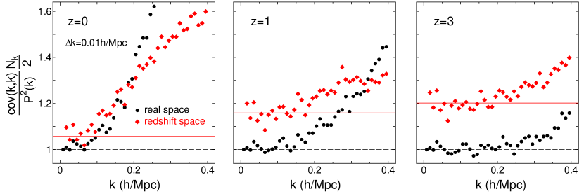
The diamond symbols in Fig.3 show the diagonal components of the redshift-space power spectrum covariances as a function of wavenumbers and at three output redshifts. The diagonal components are divided by the standard Gaussian errors, , where we have used the nonlinear power spectrum measured from the simulations. Note the difference in the normalization factor from that in Fig.1. The horizontal line in each panel shows the prefactor in Eq. (9), the amplification factor expected from the Kaiser’s formula at the large-scale limit. Therefore the deviations from the horizontal line may come from two contributions: (1) the non-Gaussian error contribution caused by nonlinear clustering and (2) the nonlinear redshift distortions such as the effect caused by the virial motions within and among halos, known as the finger-of-God effect. The circle symbols denote the simulation results for the real-space spectrum computed in a consistent way, i.e. divided by the nonlinear spectrum. The nonlinear effects on the covariance become more significant with increasing wavenumber and at lower redshifts. Interestingly, however, comparing the real- and redshift-space results manifests that the relative importance of the non-Gaussian covariances is weaker in redshift space, implying that the finger-of-God redshift distortions at small length scales more preferentially suppress the covariance amplitudes than the power spectrum amplitudes (also see Meiksin & White 1999).
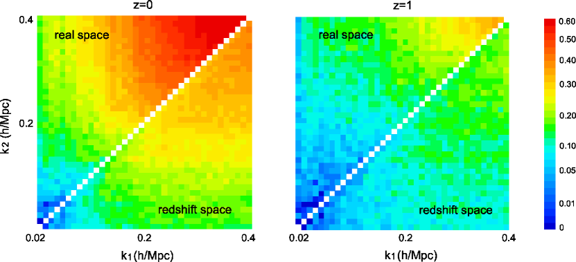
Fig.4 shows both the off-diagonal components of the covariances in real space (the left-upper elements in each panel) and redshift space (right-lower), at redshifts and . The cross-correlations are more significant with increasing wavenumbers, while the correlation strengths are relatively weaker in redshift space.
5. Probability Distribution of the Power Spectrum Estimator
We have so far discussed the non-Gaussian covariance of the power spectrum estimator . It would be also intriguing to study how the nonlinear clustering causes a non-Gaussian distribution in the power spectrum estimators of a given among our 5000 realizations. For example, if the estimators have a skewed distribution, a prior knowledge on the full distribution may be needed to obtain an unbiased estimate on the ensemble averaged band power at each from a small number of realizations or a finite volume survey. Note that the power spectrum covariance simply reflects the width (variance) of the full distribution at each ’s but does not contain full information on the probability distribution.
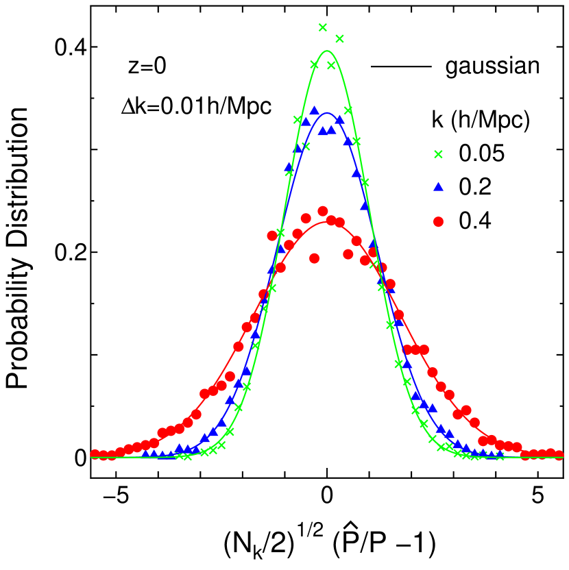
Fig. 5 shows the probability distribution of the power spectrum estimators among 5000 realizations, where we mean by “probability” that the distribution is normalized so as to give unity if the distribution is integrated over the -axis values (see below). The cross, triangle, and circle symbols show the results for and Mpc, respectively. The distribution is plotted as a function of for each such that the mean and variance of the distribution are equal to zero and unity when the power spectrum distribution obeys the linear-regime Gaussian distribution. The simulation results show that the distribution is broadened with increasing due to the stronger nonlinearities. The solid curves show the expected Gaussian distribution where its variance is set to the diagonal covariance measured from the simulations at each , i.e. the variance includes the non-Gaussian covariance contribution as given in Fig. 3. Interestingly, the simulation results are rather well approximated by the Gaussian distribution even in the non-linear regime.
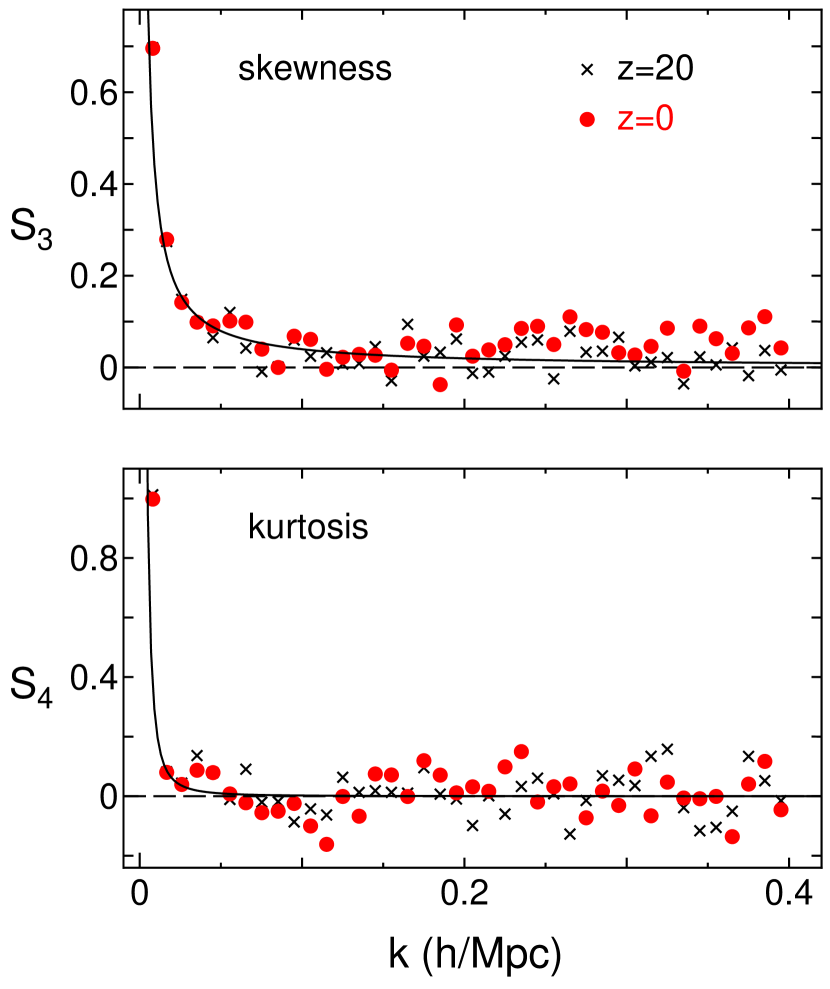
The remaining small deviations from the Gaussian distribution can be quantified by studying the skewness and kurtosis defined as
| (10) |
The and are vanishing for the Gaussian distribution. If the density field obeys the random Gaussian fields, which is a good approximation in the linear regime, the power spectrum estimator of a given (see Eq. [1]) obeys the -distribution in analogy with the CMB power spectrum (Knox 1995). In this case, as derived in Appendix B, the skewness and kurtosis can be analytically computed as
| (11) |
Fig. 6 shows the simulation results for and as a function of at and . The results are for a volume of , and the scale as and from Eq.(11). The solid curves are the theoretical predictions of Eq.(11) which well match the simulation results. Note that the skewness is positive, because the -distribution has a long tail at large ends of . Both and asymptotes to zero at high , i.e., the probability distribution approaches to a Gaussian distribution at high . The skewness grows from to through the non-linear gravitational evolution, however, its value () is very small.
6. Effects of Non-Gaussian Covariance on Signal-to-Noise Ratio
A useful way to quantify the impact of the non-Gaussian errors is to study the cumulative signal-to-noise ratio for measuring the power spectrum over a range of wavenumbers, which is also sometimes called the Fisher information content (e.g. Tegmark et al. 1997). The is defined, using the covariance (2), as
| (12) |
where denotes the inverse of the covariance matrix and the summation is up to a given maximum wavenumber . Note that the is independent of the bin width assumed, as long as the power spectrum does not vary rapidly within the bin widths.
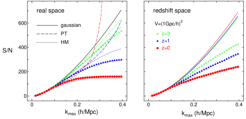
Fig.7 shows the as a function of for the spectra at and in real space (left panel) and in redshift space (right), respectively. The results for shown here are for a volume of (the scales with as ). For comparison the solid curve shows the for the Gaussian error case, which scales as independently of redshift. The simulation results show that the non-Gaussian errors degrade the . The degradation becomes more significant with increasing and at lower redshifts: for the results in real space the is degraded by up to a factor of and for and , respectively, compared to the Gaussian error case. It should be worth noting that the becomes nearly constant on and 0.3Mpc-1, i.e no gain in the even if including modes at the larger , as has been found in the previous works (Rimes & Hamilton 2005, 2006; Hamilton, Rimes & Scoccimarro 2006; Neyrinck, Szapudi & Rimes 2006; Neyrinck & Szapudi 2007; Lee & Pen 2008; Angulo et al. 2008; Smith 2008).
In the dashed curves we use the perturbation theory (PT) in Eq. (3) to calculate the covariance, while the power spectrum measured from the simulations is used for the numerator in the calculation. The PT provides a better fit to the data in the linear and weakly nonlinear regime, which is coincident within for Mpc at , Mpc at and Mpc at , respectively. However, at small scale the deviation is so large, since the theory predicts the much smaller covariance than the data as shown in Figs. 1 and 2.
The dotted curves in the left panel of Fig. 7 show the halo model results, which fairly well fit the simulation results at . At higher redshifts (), the halo model reproduces a saturation in the amplitude on the small , but underestimates the impact of the non-Gaussian errors, which is due to the underestimation in the off-diagonal elements of the covariances in the halo model (see Fig. 2).
The impact of the non-Gaussian errors on is mitigated in redshift space as in Fig. 3. Also note that the in redshift space continues to increase for the smaller scales Mpc. This is again because the nonlinear redshift distortions cause strong suppression in the non-Gaussian covariances, making the closer to the Gaussian error case.
| Redshift | Volume | Number Density | Bias |
|---|---|---|---|
| (Gpc3) | (Mpc-3) | ||
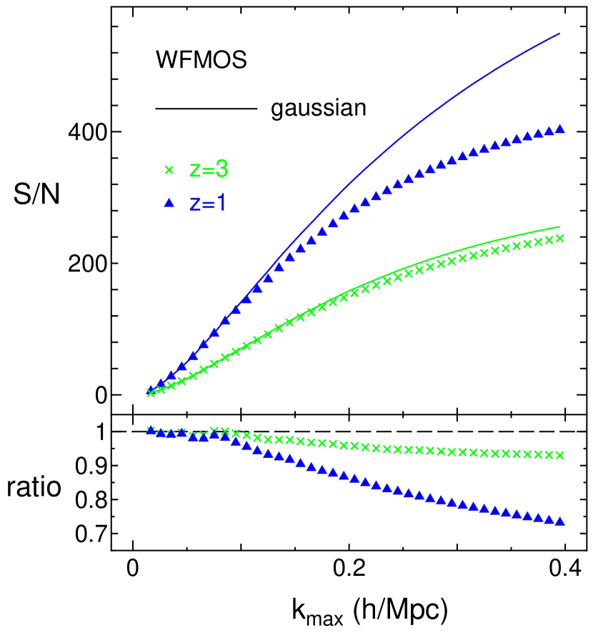
We make a more realistic estimate for the taking into account the shot noise effect of galaxies that are biased tracers of large-scale structure. To do this we consider a galaxy survey that resembles the planned survey by WFMOS (Wide-Field Fiber-Fed Optical Multi-Object Spectrograph), and assume the fiducial survey parameters given in Table 1 (see also the WFMOS feasibility report555Feasibility Study Report : http://www.gemini.edu/files /docman/science/aspen/WFMOSfeasibilityreportpublic.pdf). The target galaxies are supposed to be emission line galaxies and Lyman-break galaxies, at and , respectively. To compute the power spectrum and covariance of galaxies, we employ a linear bias model for simplicity. This assumption is not accurate since the bias is generally nonlinear and scale-dependent (Smith et al. 2007), and hence our results below just give a rough estimate on the . The bias parameters in Table 1 are chosen such that the rms density fluctuations of galaxies within a sphere of radius Mpc become (Glazebrook et al. 2005). We simply include the effects of the linear bias and the shot noise by replacing the power spectrum and the covariance in the evaluation as and , where is the mean number density of galaxies. The above replacement is done in real space.
The symbols in Fig. 8 show the simulation results in real space. The expected is found to be very significant: and 200 for the slices of and for Mpc, respectively. This implies that the WFMOS-type survey allows a precision of measuring the power spectrum amplitudes at a sub-percent level.666The Fisher information matrix for the power spectrum measurement is given as , where is a set of cosmological parameters of interest. Roughly speaking, the unmarzinalized uncertainty in estimating a parameter is given as (this exactly holds if the power spectrum amplitude, for the fixed shape, is considered as the parameter). Therefore the amplitude gives a rough estimate on the precision of parameter estimation provided the power spectrum measurement: the greater means the higher precision. The solid curves are the results obtained assuming the Gaussian covariances with the shot noise contribution, which do not scale as on scales where the shot noise is relevant in the covariance (). Compared with Fig. 7, one can find that the shot noise causes positive and negative effects on : it reduces the overall amplitudes of , but mitigates the degradation due to the non-Gaussian errors.
Since the precision of constraining individual cosmological parameters such as dark energy parameters roughly scales with the amplitude66footnotemark: 6, Fig. 8 implies that the constraining power of the fiducial WFMOS survey is degraded by the non-Gaussian errors, compared with the Gaussian error case. The impact of the non-Gaussian errors on cosmological parameter estimations will be presented in a subsequent paper (Takahashi et al. in preparation).
7. Effects of Long-Wavelength Fluctuations
We have so far employed, as usual, the simulations with periodic boundary conditions, where there is no clustering power on scales greater than the simulation box. Obviously, however, the real universe never obeys the periodic boundary condition and does contain the density perturbations of scales greater than a surveyed volume. In particular, Rimes & Hamilton (2006) pointed out a new source of the non-Gaussian errors that inevitably arises when the power spectrum is estimated from a finite-size volume, called the beat-coupling (BC) effect (2006; also see Hamilton, Rimes & Scoccimarro 2006; Sefusatti et al. 2006). If the survey region is embedded in a large-scale overdensity or underdensity region, then the small scale fluctuations we measure may have grown more rapidly or slowly than the ensemble average. There are thus non-vanishing correlations of the small-scale fluctuations with the unseen large-scale fluctuations. This physical correlations may add uncertainties in measuring the power spectrum on scales of interest.
In this section, therefore, we study how the periodic boundary conditions and the density perturbations larger than a survey volume (the volume where the Fourier transform is performed) affect the power spectrum estimation and the covariance. For this purpose we study the following three cases:
-
Case 1:
We first divide each simulation region of Gpc3 into eight cubic sub-boxes of equal volume. Each sub-box has a volume of Mpc and contains about particles. We then randomly select only one sub-box and use the particle distribution to resemble the density perturbation field. The density perturbation field outside the sub-box is zero-padded within the whole box of Gpc3. The mean mass density is computed from the number of the particles within the sub-box. Then we perform the FFT of 5123 grids for the whole box to estimate the power spectrum.
-
Case 2:
Similar to Case 1, but the FFT of 2563 grids is performed only within the sub-box of volume (Mpc that contains the -body particles (therefore no zero-padded region).
-
Case 3:
We run new simulations of volume Mpc using particles and employing the periodic boundary condition. Then the power spectrum is estimated from the whole box using the FFT of 2563 grids.
Note that the effective mass and spatial resolutions are the same in all the cases. We use 400 realizations for each case. Cases 1 and 2 do not employ the periodic boundary condition and contain the density fluctuations larger than the FFT-used volume in structure formation. However, these two cases are different in that the fundamental mode of Fourier transform, given as ( is the size of FFT volume), is smaller in Case 1 by factor 2 than in Case 2. Therefore the density fluctuation field is sampled by the finner Fourier modes in Case 1. Also note that Case 1 corresponds to a case that the FFT transform is applied to a survey with complex geometry. Case 3 has the periodic boundary condition, and is equivalent to the procedure we have employed up to the preceding section. By comparing these three cases, we will below address the effects of the periodic boundary condition, the finite Fourier sampling and the beat-coupling effect.
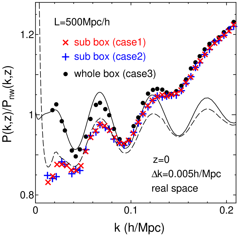
Fig. 9 shows the real-space power spectra at , estimated according to the procedures described above, where the simulated power spectra are divided by the non-wiggle linear power spectrum in Eisenstein & Hu (1999) for illustrative purpose. The cross, plus and dotted symbols are the results for Cases 1, 2 and 3, respectively. All the results agree well on scales Mpc-1. However, the results for Cases 1 and 2, which do not impose the periodic boundary condition, underestimate the power spectrum amplitudes at the linear regime Mpc-1 by up to . This is because the non-periodic density fluctuation field is expanded by the FFT transform that has periodic basis eigenfunctions within the box size (see Sirko 2005 for the similar discussion). This underestimation can be corrected for if the Fourier kernel of the non-periodic field is properly taken into account. The dashed curve is the linear power spectrum convolved with the window function which is given as inside (outside) the sub box:
| (13) |
The window function in Fourier space is
| (14) |
with Mpc. The dashed curve is the spherical averaged power spectrum, , which reproduces the dumping of the power spectrum at Mpc.
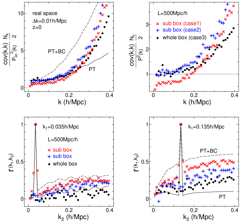

Fig.10 compares the power spectrum covariances. The top two panels show the diagonal parts normalized by the linear power spectrum (upper-left) and the spectrum measured from simulations (upper-right), which are similar to Figs.1 and 3, respectively. The number of modes in the vertical axis is used for the box for all the cases. First, comparing the results for Cases 2 and 3, we find that there are stronger non-Gaussian errors at Mpc-1 for Case 2: the presence of the density fluctuations larger than the survey volume, as in the real universe, increases the non-Gaussian error strengths due to the mode-coupling between the large- and small-scale density fluctuations. Next, let’s compare Case 1 with Cases 2 and 3. The results for Case 1 are clearly smaller than Cases 2 and 3 even at the linear scales such as Mpc-1, but show stronger non-Gaussian errors than Case 3 on the large ’s as in Case 2. The differences between Cases 1 and 2 are caused by the presence of the zero-padded regions within the FFT volume and the finer Fourier sampling. For Case 1, the density perturbations of scales comparable to the FFT volume are non-periodic due to a mixture of the zero-padded region and the N-body particle distribution in the sub-volume. Therefore, the Fourier transform causes artificial cross-correlations between the Fourier modes of different ’s even in the linear regime. Due to the cross-correlations, the off-diagonal covariances are amplified as shown in the lower panels, while the diagonal covariances are relatively suppressed.
The behaviors of the off-diagonal covariances shown in the lower panels are similarly understood. Comparing the three cases one can find that the long-wavelength fluctuation effect and the zero-padding plus the finer Fourier sampling cause stronger cross-correlations between the spectra of different ’s over the range of we have considered.
More important results are given in Figs. 11, showing the cumulative values for Cases 1, 2 and 3, computed properly taking into account the covariances in Figs. 10. Each panel shows the results at redshifts of (left), (center) and (right). First of all, all the results agree well with the Gaussian error case on the linear scales, Mpc-1. At the larger ’s, the results for Cases 1 and 2 show that the presence of long-wavelength fluctuations further degrades the amplitudes by 20% at redshift and by 30% at and 3, respectively, compared to the results with the periodic boundary condition (Case 3). This implies that, even for high redshifts and at the BAO scales, the additional non-Gaussian errors due to the long-wavelength fluctuation effect need to be included in the analysis for an actual survey. Interestingly, the values for Cases 1 and 2 become to agree well, even though their covariances are very different as shown in Fig. 10. This agreement is reasonable, because Cases 1 and 2 contain the similar mass density fields of same volume; therefore the amount of cosmological information to be extracted is similar. These are different only in the FFT procedures.
A full physical understanding of the complex covariance behaviors is beyond the scope of this paper. Nevertheless, it would be interesting to compare the simulation results with an analytical model. A crude model to describe the long-wavelength fluctuation effect on the non-Gaussian covariance is proposed in Hamilton et al. based on the perturbation theory (also see Takada & Jain 2008):
| (15) |
where (Mpc-1 for Cases 1 and 2). This model ignores the Fourier transform effect of the non-periodic density field and rests on a simplified assumption that the long-wavelength fluctuation effect arises from a correlation of the fundamental Fourier mode with the wavenumbers we want to measure. Developing a more accurate analytical model of the long-wavelength fluctuation effect is now in progress and will be presented elsewhere (Kayo et al. in preparation).
The solid curves in Fig. 10 show the for the Gaussian error case, and roughly explains the simulation results up to the linear regimes. The dashed curves show the PT model predictions including the BC effect modeled by Eq. (15), which are intended to reproduce the results for Case 2. The dotted curves show the results obtained when the halo model contribution to the covariance is further included. These analytic models do not describe the complex behaviors of the diagonal and off-diagonal covariances seen in the simulations. Also the simulation results for cannot be explained by the analytic models. The analytical model in Eq.(15) overestimates the beat-coupling effect. This conclusion agrees with a recent study of Reid, Spergel & Bode (2008), where they showed that the simulation results are fairly well explained if Eq. (15) reduced by a factor 3 is added to the Gaussian covariance.
8. Discussion and Conclusion
Having well-calibrated, accurate covariances of the power spectrum is clearly needed in order to obtain unbiased, robust cosmological constraints from ongoing/future BAO experiments. In previous studies, the covariance matrix is calculated either by using analytic models which cannot be applied to fully nonlinear regimes, or by using a limited number of simulation realizations (Scoccimarro et al. 1999; Meiksin & White 1999; Rimes & Hamilton 2005 and Neyrinck & Szapudi 2008). In this paper, we used a very large number () of the realizations to study the power spectrum covariances, allowing us to achieve the convergence at a few % level.
We have carefully studied how the non-Gaussian error contributions to the covariance vary with scales and redshifts for the concordance CDM model. As expected in the CDM model, the non-Gaussian errors become more significant on smaller length scales and at lower redshifts. For redshifts , 1 and , the cumulative signal-to-noise () ratios for measuring the power spectrum over Mpc-1 are degraded due to the non-Gaussian errors by a factor of 1.3, 2.3 and 4, respectively, compared to the Gaussian error cases. This degradation is slightly mitigated in redshift space because the nonlinear redshift distortions cause a stronger suppression in the covariance amplitudes than in the power spectrum amplitudes.
We also estimated how the density fluctuations of scales greater than a survey size cause additional non-Gaussian errors via the correlations with the fluctuations we want to measure, which inevitably arises for a finite-size survey – the so-called beat-coupling effect. This effect disappears when estimating the power spectrum covariances from simulations with the periodic boundary condition. Thus we rather used the sub-region of the original simulation to estimate the new non-Gaussian errors, and showed that the beat coupling effect can be important even in the weakly nonlinear regime and for high redshifts: it further suppresses the by at , and at and , respectively. However, the behaviors of these non-Gaussian errors cannot be described by the naive analytic models with and without the beat-coupling effect. Therefore it will be worth exploring a more accurate analytical model of the non-Gaussian covariances. Such a model will help us to obtain physical interpretation and to calibrate the derived covariance for arbitrary cosmological models and survey parameters (Kayo et al. in preparation).
We also studied the probability distribution of the power spectrum estimators among the 5000 realizations. We found that the distribution is nearly Gaussian even in the nonlinear regime. More precisely, the mean of the power spectrum estimators is not largely biased from the ensemble average, and the scatters are well given by the diagonal power spectrum covariance at a given wavenumber.
A more important question would be how an actual galaxy survey is affected by the non-Gaussian errors. For this purpose, we made a simplified estimate on the expected for a WFMOS-type survey, further taking into account the shot noise contamination to the covariance due to finite number densities of galaxies. Since the shot noise contributes only to the Gaussian errors (in an ideal case), including the shot noise not only reduces the total amplitude, but also mitigates the influence of the non-Gaussian errors. Thus the impact of the non-Gaussian errors does vary with survey parameters. Since the precision of a given survey for constraining cosmological parameters roughly scales with the amplitude, an optimal survey design needs to be realized by taking into account the non-Gaussian errors, given the resources and observing times for a survey. Furthermore the non-Gaussian errors may cause the best-fitting parameters to be biased if the model fitting is done improperly assuming the Gaussian covariances, because the non-Gaussian errors are more significant on smaller length scales and cause correlated uncertainties between the band powers. These issues will be studied in a forthcoming paper (Takahashi et al. in preparation).
Our simulation results of the power spectrum and the covariance matrix are available as numeric tables upon request (contact takahasi@a.phys.nagoya-u.ac.jp).
Appendix A Convergence of the Covariance Matrix
It is useful to estimate the necessary number of realizations to achieve a desired accuracy for estimating the power spectrum covariance. In this appendix, we examine the numerical convergence of the covariance estimation. Let us define the dispersion of the covariance matrix as
| (A1) |
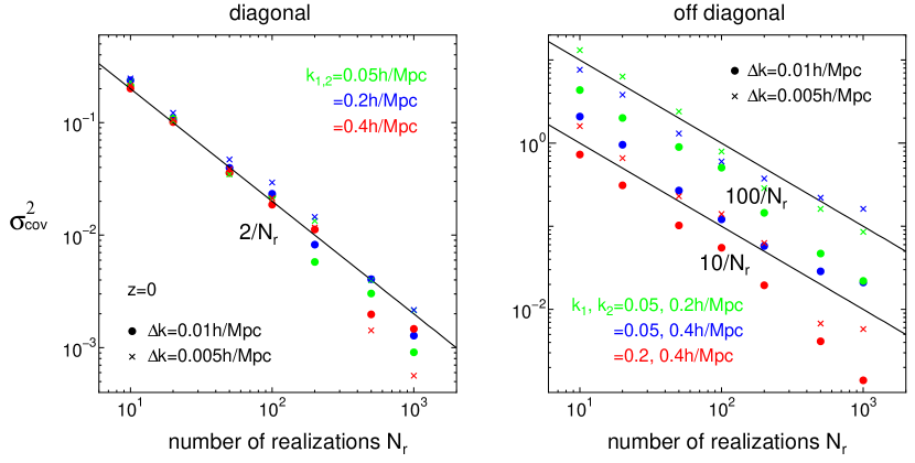
Here, is the ensemble average over all the realizations, while is the covariance estimated from a subset of the realizations whose number is denoted as . Fig. 12 shows the dispersion in Eq.(A1) as a function of the number of realizations . The left panel is for the diagonal elements, and each color symbols correspond to (green), (blue) and Mpc (red) with the bin width (circles) and Mpc (crosses). The solid line represents which fits the data very well. Hence, we numerically find the scaling of the dispersion given by
| (A2) |
Note that the above result is independent of the scale , the bin width and the simulation box volume.
The right panel is for the off-diagonal elements for , and Mpc, respectively. The solid lines represent and . Similar to the diagonal parts, we obtain
| (A3) |
for . Here () are the numbers of modes available for the bins with the bin width, and the proportionality factor would depend on the scale . The analytical derivation for Eqs.(A2) and (A3) will be presented in Kayo et al. (in preparation).
Appendix B Probability Distribution of the Power Spectrum Estimator in Gaussian Limit
In the linear regime, the real and imaginary parts of the density fluctuation ( and ) follow the Gaussian distribution with mean and dispersion . The power spectrum estimator for a given realization is the summation of the squared Gaussian fluctuations, ). Then the distribution of obeys the chi-square distribution (e.g. Abramowitz & Stegun 1970):
| (B1) |
for and for . Its mean and dispersion are and , respectively. The skewness and kurtosis are given in Eq.(11). In the limit of it reduces to the Gaussian distribution. The factor two in the number of modes arises because and are not independent.
References
- Abramowitz & Stegun (1970) Abramowitz, M. & Stegun, I.A., 1970, Handbook of Mathematical Functions, Dover Publications
- Angulo et al. (2007) Angulo, R.E., Baugh, C.M., Frenk, C.S., & Lacey, C.G., 2008, MNRAS, 383, 755
- Bernardeau et al. (2002) Bernardeau, F., Colombi, S., Gaztanaga, E., & Scoccimarro, R., 2002 Physics Reports, 367, 1
- Benitez et al. (2008) Benitez, N. et al., 2008, ApJ, 691, 241
- Blake & Glazebrook (2003) Blake, C. & Glazebrook, K., 2003, ApJ, 594, 665
- Cole et al. (2005) Cole, S., et al., 2005, MNRAS, 362, 505
- Cooray & Hu (2001) Cooray, A. & Hu, W., 2001, ApJ, 554, 56
- Cooray & Sheth (2002) Cooray, A. & Sheth, R., 2002, Physics Reports, 372, 1
- Crocce & Scoccimarro (2006) Crocce, M. & Scoccimarro, R., 2006, PRD, 73, 063519
- Crocce & Scoccimarro (2008) Crocce, M. & Scoccimarro, R., 2008, PRD, 77, 023533
- Eifler, Schneider & Hartlap (2008) Eifler, T., Schneider, P. & Hartlap, J., 2008, submitted to A&A, arXiv:0810.4254
- Eisenstein, Hu & Tegmark (1998) Eisenstein, D.J., Hu, W. & Tegmark, M., 1998, ApJ, 504, L57
- Eisenstein & Hu (1999) Eisenstein, D.J. & Hu, W., 1999, ApJ, 511, 5
- Eisenstein et al. (2005) Eisenstein, D.J. et al., 2005, ApJ, 633, 560
- Feldman, Kaiser & Peacock (1994) Feldman, H.A., Kaiser, N. & Peacock, J.A., 1994, ApJ, 426, 23
- Gaztanaga, Cabre & Hui (2008) Gaztanaga, E., Cabre, A. & Hui, L., 2008, arXiv:0807.3551
- Glazebrook et al. (05) Glazebrook, K. et al., 2005, astro-ph/0507457
- Guzik, Bernstein & Smith (2007) Guzik, J., Bernstein, G. & Smith, R.E., 2007, MNRAS, 375, 1329
- Habib et al. (2007) Habib, S., Heitmann, K., Higdon, D., Nakhleh, C., & Williams, B., 2007, PRD, 76, 083503
- Hamilton, Rimes & Scoccimarro (2006) Hamilton, A.J.S., Rimes, C.D. & Scoccimarro, R., 2006, MNRAS, 371, 1188
- Hockney & Eastwood (1988) Hockney, R.W. & Eastwood, J.W., 1988, Computer Simulations Using Particles (New York: Taylor & Francis Group)
- Huff et al. (2007) Huff, E., et al., 2007, Astroparticle Physics, 26, 351
- Ichiki, Takada & Takahashi (2009) Ichiki, K., Takada, M. & Takahashi, T., 2009, PRD, 79, 023520
- Jain & Bertschinger (1994) Jain, B. & Bertschinger, E., 1994, ApJ, 431, 495
- Jeong & Komatsu (2006) Jeong, D. & Komatsu, E., 2006, ApJ, 651, 619
- Jeong & Komatsu (2009) Jeong, D. & Komatsu, E., 2009, ApJ, 691, 569
- Kaiser (1987) Kaiser, N., 1987, MNRAS, 227, 1
- Knox (1995) Knox, L., 1995, Phys. Rev. D, 52, 4307
- Lee & Pen (2008) Lee, J. & Pen, U.-L., 2008, ApJL, 686, 1
- Lewis, Challinor & Lasenby (2000) Lewis, A., Challinor, A. & Lasenby, A., 2000, ApJ, 538, 473
- Ma & Fry (2000) Ma, C.-P., & Fry, J. N., 2000, ApJ, 543, 503
- Makino, Sasaki & Suto (1992) Makino, N., Sasaki, M. & Suto, Y., 1992, PRD, 46, 585
- Matarrese & Pietroni (2007) Matarrese, S. & Pietroni, M., 2007, JCAP 0706:026
- Matarrese & Pietroni (2008) Matarrese, S. & Pietroni, M., 2008, Mod. Phys. Lett. A, 23, 25
- Matsubara (2004) Matsubara, T., 2004, ApJ, 615, 573
- (36) Matsubara, T., 2008a, PRD, 77, 063530
- (37) Matsubara, T., 2008b, PRD, 78, 083519
- Meiksin, White & Peacock (1999) Meiksin, T., White, M. & Peacock, J.A., 1999, MNRAS, 304..851
- Meiksin & White (1999) Meiksin, T. & White, M., 1999, MNRAS, 308, 1179
- McDonald (2007) McDonald, P., 2007, PRD, 75, 043514
- Mo & White (1996) Mo, H.J. & White, S.D.M., 1996, MNRAS, 282, 347
- Mo, Jing & White (1997) Mo, H.J., Jing, Y.P. & White, S.D.M., 1997, MNRAS, 284, 189
- Navarro, Frenk & White (1997) Navarro, J., Frenk, C. & White, S.D.M., 1997, ApJ, 490, 493
- Neyrinck, Szapudi & Rimes (2006) Neyrinck, M.C., Szapudi, I. & Rimes, C.D., 2006, MNRAS, 370, L66
- Neyrinck & Szapudi (2007) Neyrinck, M.C. & Szapudi, I., 2007, MNRAS, 375, L51
- Neyrinck & Szapudi (2008) Neyrinck, M.C. & Szapudi, I., 2008, MNRAS, 384, 1221
- Nishimichi et al. (2007) Nishimichi, T., et al., 2007, PASJ, 59, 1049
- Nishimichi et al. (2008) Nishimichi, T., et al., 2008, PASJ in press, arXiv0810.0813
- Nomura, Yamamoto & Nishimichi (2008) Nomura, H., Yamamoto, K. & Nishimichi, T., 2008, JCAP, 10, 031
- Okumura et al. (2007) Okumura, T., et al., 2008, ApJ, 676, 889
- Peacock & Smith (2000) Peacock, J. A., & Smith, R. E., 2000, MNRAS, 318, 1144
- (52) Percival, W.J., et al., 2007, MNRAS, 381, 1053
- Pietroni (2008) Pietroni M., 2008, JCAP 0810:036
- Rassat et al. (2008) Rassat, A. et al., 2008, submitted to MNRAS, arXiv:0810.0003
- Reid, Spergel & Bode (2008) Reid, B.A., Spergel, D.N. & Bode, P., 2008, submitted to ApJ, arXiv:0811.1025
- Rimes & Hamilton (2005) Rimes, C.D. & Hamilton, A.J.S., 2005, MNRAS, 360, L82
- Rimes & Hamilton (2006) Rimes, C.D. & Hamilton, A.J.S., 2006, MNRAS, 371, 1205
- Sanchez, Baugh & Angulo (2008) Sanchez, A.G., Baugh, C.M. & Angulo, R., 2008, MNRAS, 390, 1470
- Sanchez et al. (2009) Sanchez, A.G., et al., 2009, submitted to MNRAS, arXiv:0901.2570
- Scoccimarro, Zaldarriaga & Hui (1999) Scoccimarro, R., Zaldarriaga, M. & Hui, L., 1999, ApJ, 527, 1
- Scoccimarro & Sheth (2002) Scoccimarro, R. & Sheth, R.K., 2002, MNRAS, 329, 629
- Scoccimarro (2004) Scoccimarro, R., 2004, PRD, 70, 083007
- Sefusatti, Crocce, Pueblas & Scoccimarro (2006) Sefusatti, E., Crocce, M., Pueblas, S. & Scoccimarro, R., 2006, PRD, 74, 023522
- Seljak (2000) Seljak, U., 2000, MNRAS, 318, 203
- Seo & Eisenstein (2003) Seo, H.J. & Eisenstein, D.J., 2003, ApJ, 598, 720
- Seo & Eisenstein (2005) Seo, H.J. & Eisenstein, D.J., 2005, ApJ, 633, 575
- Seo et al. (2008) Seo, H.J. Siegel, E.R., Eisenstein, D.J. & White M., 2008, ApJ, 686, 13
- Sheth & Tormen (1999) Sheth, R.K. & Tormen, G., 1999, MNRAS, 308, 119
- Sirko (2005) Sirko, E., 2005, ApJ, 634, 728
- Smith, Scoccimarro & Sheth (2007) Smith, R.E., Scoccimarro, R. & Sheth, R.K., 2007, PRD, 75, 3512
- Smith, Scoccimarro & Sheth (2008) Smith, R.E., Scoccimarro, R. & Sheth, R.K., 2008, PRD, 77, 3525
- Smith (2008) Smith, R.E., 2008, submitted to MNRAS, arXiv:0810.1960
- Spergel et al. (2007) Spergel, D.N., et al., 2007, ApJ, 170, 377
- Springel, Yoshida & White (2001) Springel, V., Yoshida, N. & White, S.D.M., 2001, New Astronomy, 6, 79
- Springel (2005) Springel, V., 2005, MNRAS, 364, 1105
- Takada & Jain (2003) Takada, M., & Jain, B., 2003, MNRAS, 340, 580
- Takada & Jain (2008) Takada, M. & Jain, B., 2008, MNRAS in press, arXiv:0810.4170
- Takahashi et al. (2008) Takahashi, R., et al., 2008, MNRAS, 389, 1675
- Takahashi (2008) Takahashi, R., 2008, Progress of Theoretical Physics, 120, 549
- Taruya & Hiramatsu (2008) Taruya, A. & Hiramatsu, T., 2008, ApJ, 674, 617
- Tegmark, Taylor & Heavens (1997) Tegmark, M., Taylor, A.N. & Heavens, A.F., 1997, ApJ, 480, 22