Deep Spectroscopy of Ultra-Strong Emission Line Galaxies

Abstract

Ultra-strong emission-line galaxies (USELs) with extremely high equivalent widths (EW(H$\beta)\geq 30$ Å) can be used to pick out galaxies of extremely low metallicity in the $z=0-1$ redshift range. Large numbers of these objects are easily detected in deep narrow band searches and, since most have detectable [O III]$\lambda$4363, their metallicities can be determined using the direct method. These large samples hold out the possibility for determining whether there is a metallicity floor for the galaxy population. In this, the second of our papers on the topic, we describe the results of an extensive spectroscopic follow-up of the Kakazu et al. (2007) catalog of 542 USELs carried out with the DEIMOS spectrograph on Keck. We have obtained high S/N spectra of 348 galaxies. The two lowest metallicity galaxies in our sample have 12+log(O/H) = 6.97$\pm 0.17$ and 7.25$\pm 0.03$ – values comparable to the lowest metallicity galaxies found to date. We determine an empirical relation between metallicity and the R23 parameter for our sample, and we compare to this to the relationship for low redshift galaxies. The determined metallicity-luminosity relation for this sample is compared with that of magnitude selected samples in the same redshift range. The emission line selected galaxies show a metal-luminosity relation where the metallicity decreases with luminosity and they appear to define the lower bound of the galaxy metallicity distribution at a given continuum luminosity. We also compute the H$\alpha$ luminosity function of the USELs as a function of redshift and use this to compute an upper bound on the Ly$\alpha$ emitter luminosity function over the $z=0-1$ redshift range.

1. Introduction

Developing a large sample of low metallicity galaxies is of considerable interest for clues it can provide to the early stages of galaxy formation and chemical enrichment — such as whether forming galaxies have a baseline metallicity that reflects the early chemical enrichment of the intergalactic medium. The most metal-poor systems currently known are the low redshift blue compact emission-line galaxies such as I Zw 18 and SBS 0335-052W with measured 12+log (O/H) of $\sim 7.1-7.2$ (Sargent & Searle 1970; Thuan & Izotov 2005; Izotov et al. 2005). However, despite enormous efforts, only a few dozen xMPGs (objects with (12+log (O/H) $<7.65$ or $Z<Z_{\sun}/12$; Kniazev et al. 2003; Izotov et al. 2006a) are known (e.g., Oey, 2006; Izotov, 2006b). There are too few of these for detailed studies of the metallicity distribution function.

In the first paper of the present series we showed that large samples of low metallicity objects can be found by searching for ultra-strong emission-line galaxies (USELs) using very deep narrowband surveys (Kakazu et al., 2007). The narrowband method has many advantages; it is an efficient way to develop very large samples of objects and, since it probes to much deeper line-flux limits than objective prism or continuum surveys, we can study populations out to near redshift $z\sim 1$ where the cosmic star formation rates peak.

In the present work we report on the detailed spectroscopic follow-up of the catalog of 542 USEL galaxies given in Kakazu et al. (2007). The Kakazu et al. sample was chosen from a set of narrowband images obtained with the SuprimeCam mosaic CCD camera on the Subaru 8.2-m using two $\sim$120 Å (FWHM) filters centered at nominal wavelengths of 8150 Å and 9140 Å in regions of low sky background between the OH bands. The total covered area is 0.5 square degrees. The catalog consists of all objects with narrow band magnitudes less than 25 and a narrow band excess of 0.8 magnitudes for the 8150 Å filter and of 1.0 magnitudes in the 9140 Å filter compared to their respective reference continuum bands. The sample should contain all galaxies in the fields with observed frame equivalent widths significantly greater than 120Å and 180Å in the two filters, and with line fluxes above $\sim 1.5\times 10^{-17}$ erg cm^-2 s^-1.

Spectroscopic redshifts have now been obtained for 299 of these galaxies using multi-object masks with the DEIMOS spectrograph (Faber et al., 2003) on the 10-m Keck II telescope. The observations, flux calibration, and equivalent width measurements are discussed in $\S 2$, where the resulting measured line ratios are also described. In $\S 3$ we analyse the metallicities and describe an empirical relation for the metallicity as a function of the R23 parameter, which we compare with low redshift determinations of the relation. The distribution of metallicities as a function of the properties of the galaxies is given in $\S 4$ where we also compare the results with those in magnitude selected samples at the same redshift. In $\S 5$ we show that the results can be used to place upper limits on the Lyman alpha emitter (LAE) luminosity function in the $z=0-1$ redshift range, and compare this both with the local GALEX measurement of Deharveng et al. (2008) and with higher redshift LAE functions. A final summary discussion is given in $\S 6$. We use a standard $H_{0}$ = 70 km s^-1 Mpc^-1, $\Omega_{m}$ = 0.3, $\Omega_{\Lambda}$ = 0.7 cosmology throughout the paper.

Figure 1.— Redshift versus narrow band magnitude in the selection filter. The lower histogram (blue line) shows the fraction of objects in the magnitude range which have either not been observed or not been identified.

2. Spectrosopic observations

(Kakazu et al., 2007) reported spectroscopic observations for 161 USELs from their sample. These spectra were obtained using the Deep Extragalactic Imaging Multi-Object Spectrograph (DEIMOS; Faber et al. 2003) on the Keck II 10-m telescope in a series of runs between 2003 and 2006. Over the 2007 and 2008 period we have roughly doubled this spectroscopic sample and have also significantly deepened the spectra of many of the objects that had previously been observed.

In order to provide the widest possible wavelength coverage the observations were primarily made with the ZD600 $\ell$/mm grating. We used $1^{\prime\prime}$ wide slitlets which in this configuration give a resolution is 4.5 Å, sufficient to distinguish the [O II]$\lambda$3727 doublet structure. This allows us to easily identify [O II]$\lambda$3727 emitters where often the [O II]$\lambda$3727 doublet is the only emission feature. The spectra cover a wavelength range of approximately 5000 Å with an average central wavelength of $7200$ Å, though the exact wavelength range for each spectrum depends on the slit position with respect to the center of the mask along the dispersion direction. The observations were not generally taken at the parallactic angle, since this was determined by the mask orientation, so considerable care must be taken in measuring line fluxes, as we discuss below. Each $\sim 1$ hr exposure was broken into three subsets, with the objects stepped along the slit by $1.5^{\prime\prime}$ in each direction. Some USELs were observed multiple times, resulting in total exposure times of up to $10$ hours. The two-dimensional spectra were reduced following the procedure described in Cowie et al. (1996) and the final one-dimensional spectra were extracted using a profile weighting based on the strongest emission line in the spectrum.

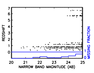
Our primary goal was to obtain a nearly complete set of spectra for the 200 objects in the catalog with narrow-band magnitudes brighter than 24, since, for these brighter objects, we can obtain high quality spectra suitable for detailed analysis. However, we also observed a large number of the galaxies with magnitudes in the 24-25 range. We have now observed 171 of the galaxies brighter than 24. Nearly all of the bright emission line candidates which were observed were identified (164 of the 171 objects). However, three of the objects in the sample are stars where the absorption line structure mimics emission in the band. The redshift distribution of the sample and the fraction of objects which have so far been identified is shown as a function of the narrow-band magnitude in Figure 1.

Figure 2.— Redshift distribution of the spectroscopically observed sample. The peaks correspond to the positions at which the strong emission lines cross the two filters. Thus there are galaxies at $z=0.6$ and $z=0.8$ corresponding to the [O III]$\lambda$5007 line lying in the $8150$ Å and $9140$ Å filters respectively.

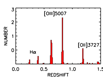
The narrow-band emission-line selection produces a mixture of objects corresponding to H$\alpha$, [O III]$\lambda$5007, and [O II]$\lambda$3727 and, at the faintest magnitudes ($>24$), high redshift ($z>5$) Ly$\alpha$ emitters. There are almost no high redshift Lyman alpha emitters at magnitudes brighter than 24. The distribution of the redshifts for objects other than the LAEs is shown in Figure 2. The largest fraction of objects corresponds to cases where the [O III]$\lambda$5007 line lies in the narrow band filters. For the present work only the objects selected in [O III] or H$\alpha$ are of interest, since we cannot determine the metallicities or the Balmer line strengths of the [O II] selected samples without futher near infrared spectroscopy. Our final sample of galaxies therefore consists of 214 galaxies with redshifts between zero and one of which 189 are chosen with [O III] and 25 with H$\alpha$. 125 of these have narrow band magnitudes brighter than AB=24.

Figure 3.— Portions of the spectrum of the the lowest metallicity galaxy in the sample showing detected emission lines. This is object 29 in the Kakazu et al. (2007) catalog of objects selected in the NB912 filter. It lies at a redshift of 0.3931. The emission line features are labeled and marked with the solid lines. In panels (a) and (b) we have increased the scale of the vertical axis to show the extremely strong H$\alpha$, [O III], and H$\beta$ lines. The [O II] line is only marginally detected in this spectrum and the two [N II] lines in panel (a) are not seen.

3. Flux Calibrations

Generally our spectra were not obtained at the parallactic angle since this is determined by the DEIMOS mask orientation required to maximize object placement in slits over the entire mask field. Therefore, flux calibration using standard stars is problematic because of atmospheric refraction effects, and special care must be taken for the flux calibration. A much more extensive discussion can be found in Kakazu et al. (2007) but here we focus only on measurements of the relative line fluxes from the spectra which we require for the metallicity measurements.

Figure 4.— Portions of the spectrum of the second lowest metallicity galaxy in the sample showing detected emission lines. This is object 269 in the Kakazu et al. (2007) catalog of objects selected in the NB912 filter. It lies at a redshift of 0.8175. In (a) we have increased the scale of the vertical axis to show the extremely strong [O III] and H$\beta$ lines. The emission line features are labeled and marked with the solid lines.

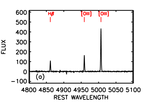
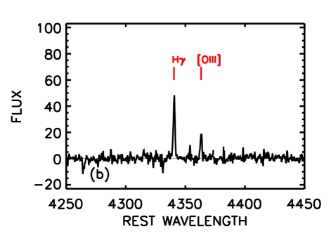
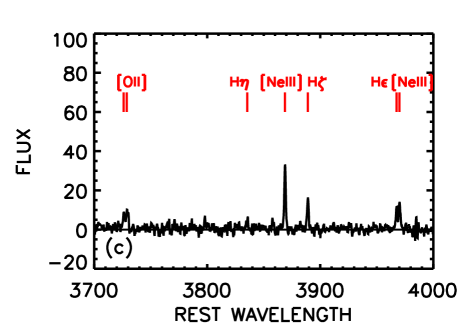
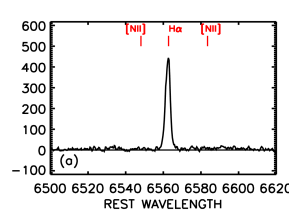
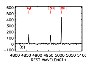
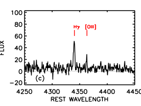
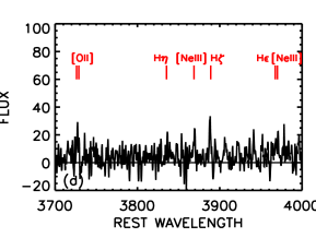
The spectra were initially relatively calibrated using the measured instrument response. Portions of the spectra of the two lowest metallicity galaxies in the sample are shown in Figures 3 and 4. Relative line fluxes can be robustly measured from the spectra without flux calibration as long as we restrict the line measurements to short wavelength ranges where the DEIMOS response is essentially constant. For example, one can assume that the responses of neighboring lines (e.g. [O III]$\lambda$4959 and [O III]$\lambda$5007) are the same and therefore one can measure the flux ratio without calibration. The present problem is considerably simplified by the presence of the H$\beta$ line near [O III]$\lambda$4959 and [O III]$\lambda$5007 (Figure 3(b) and Figure 4(a)) and the H$\gamma$ line near [O III]$\lambda$4363 (Figure 3(c) and Figure 4(b)). For these lines, and also for the [N II]$\lambda$6584 line (Figure 3(a)) we can therefore use the Balmer line ratios to provide extinction corrected flux ratios for the metal lines. To calibrate these lines, we used neighboring Balmer lines with the assumption of Case B recombination conditions. We cannot so easily do this near [O II]$\lambda$3727 where the Balmer lines are weak and in some cases contaminated (Figure 3(d) and Figure 4(c)). Fortunately the [O II]$\lambda$3727 is generally extremely weak in the spectra and the uncertainty in the calibration has little effect on the metal determination.

For each spectrum we fitted a standard set of lines. For the stronger lines we used a full Gaussian fit together with a linear fit to the continuum baseline. For weaker lines we held the full width constant using the value measured in the stronger lines and set the central wavelength to the nominal redshifted value. The [O II]$\lambda$3727 line was fitted with two Gaussians with the appropriate wavelength separation. We also measured the noise as a function of wavelength by fitting to random positions in the spectrum and computing the dispersion in the results.

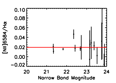
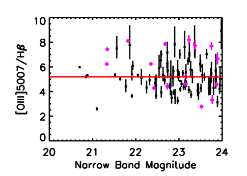
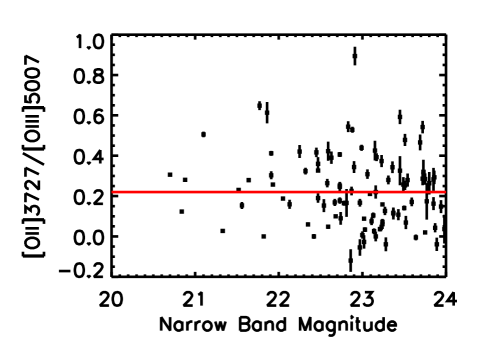
The [N II]$\lambda$6584/H$\alpha$, [O III]$\lambda$5007/H$\beta$, and [O II]$\lambda$3727/[O III]$\lambda$5007 ratios are shown as a function of the narrow band magnitude in the selection filter in Figure 5. The population is relatively uniform in its line properties. Nearly all of the galaxies have weak [N II]/H$\alpha$, (a median ratio of 0.02), weak [O II]$\lambda$3727 relative to [O III]$\lambda$5007, (a median ratio of 0.22), and strong [O III]$\lambda$5007/H$\beta$, (a median ratio of 5.2). There seems to be little difference between the H$\alpha$ selected population (shown with purple diamonds in Figure 5b) and the [O III] selected population (shown with black squares). The very weak [N II] lines, in combination with the very strong [O III], show that these galaxies are not excited by active galactic nuclei, and that the galaxies have very high ionization parameters and low metallicity, as we shall quantify in the next section.

4. Galaxy Metallicities

The spectra are of variable quality, reflecting the range of magnitudes and exposure times, and, in order to measure the metallicities, we need very high signal to noise observations. It is also important that the Balmer lines are well detected since our flux calibrations rely on the neighboring Balmer lines. We therefore restrict ourselves to emitters whose H$\gamma$ line fluxes are detected above the ten sigma level. Among the 25 H$\alpha$ selected emitters in our total spectroscopic sample there are 8 sources with spectra of sufficient quality for the metallicity analysis, and among the 189 sources selected using [O III]$\lambda$5007 there are 23 such sources, giving a total sample of 31 sources for the metallicity analysis.

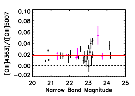
As we illustrate in Figure 6, nearly all of these sources are detected in the [O III]$\lambda$4363 auroral line. Of the 31 sources, 23 are detected above the 3 sigma level and 9 above the 5 sigma level. The median value of the ratio of the [O III]$\lambda$4363 auroral line to the [O III]$\lambda$5007 line is 0.018 for the 31 objects and there is no indication that the values seen in spectra selected with the H$\alpha$ line, which are shown by the purple diamonds in Figure 6, are any different from those selected with [O III]$\lambda$5007 which are shown by the black squares.

Figure 5.— Flux ratios of [N II]$\lambda$6584/H$\alpha$ (panel a), [O III]$\lambda$5007/H$\beta$ (b), and [O II]$\lambda$3727/[O III]$\lambda$5007 (c) computed from the spectra. The line ratios are only plotted for spectra where the signal to noise of the H$\beta$ line is greater than five. In a small number of cases the line fluxes of the weak [N II]$\lambda$6584 and [O II]$\lambda$3727 lines in the spectra scatter to negative values. The data are plotted against the narrow band magnitude and the error bars are one sigma. H$\alpha$ selected spectra are shown with purple diamonds in panel (b). The red solid curves show the median values in the sample.

Figure 6.— Ratio of the [O III]$\lambda$4363/[O III]$\lambda$5007 fluxes. The data are plotted against the narrow band magnitude and the error bars are one sigma. Only spectra where the signal to noise of the H$\gamma$ line is above ten are included. The values for the H$\alpha$ selected spectra are shown with purple diamonds and for the [O III]$\lambda$5007 selected spectra with black squares. The red solid line show the median value in the combined sample of 31 galaxies. The black solid line shows the zero ratio. Only three of the sources do not have [O III]$\lambda$4363 detected above the one sigma level.

The presence of [O III]$\lambda$4363, immediately suggests that these are metal-deficient systems but, more importantly, it allows us to determine the electron temperature from the ratio of the [O III]$\lambda$4363 line to [O III]$\lambda$$\lambda$5007,4959. This procedure is often referred to as the ‘direct’ method or $T_{e}$ method (e.g., Seaton, 1975; Pagel et al., 1992; Pilyugin & Thuan, 2005; Izotov et al., 2006c). To derive $T_{e}$[O III] and the oxygen abundances, we used the Izotov et al. (2006c) formulae, which were developed with the latest atomic data and photoionization models. Using the Pagel et al. (1992) calibrations with the $T_{e}$[O II]$-$$T_{e}$[O III] relations derived by Garnett (1992), gives consistent abundances within 0.1 dex. The [S II]$\lambda\lambda$6717, 6731 lines that are usually used for the determination of the electron number density, are beyond the Keck/DEIMOS wavelength coverage for our [O III] emitters. Therefore we assumed n_e = 100 cm^-3. However the choice of electron density has little effect as electron temperature is insensitive to the electron density; indeed we get the same results even when we use n_e = 1,000 cm^-3.

The spectra of the three lowest redshift H$\alpha$ emission-line selected galaxies do not cover the [O II]$\lambda$3727 line, leaving us with a final sample of 28 galaxies for our analysis. Seven of these objects satisfy the definition of XMPGs [12 + log(O/H) $<$ 7.65; Kunth & Östlin 2000]. The lowest metallicity galaxes in the sample are KHC912-29 with 12 + log(O/H) $=6.97\pm 0.17$, and KHC912-269 which has 12 + log(O/H) $=7.25\pm 0.03$. The spectra of these two galaxies are shown in Figures 3 and 4. Their metallicities are comparable to the currently known most metal-poor galaxies [I Zw 18 and SBS0335$-$052W; 12 + log(O/H) $\sim$ 7.1 $-$ 7.2].

5. Discussion

5.1. Metallicity and the ionization parameter

Figure 7 shows the electron temperature sensitive line ratio, [O III]($\lambda$4363)/[O III]$\lambda$5007 versus [O II]$\lambda$3727/[O III]$\lambda$5007. If we have an estimate of the metallicity, as in the present case, we can use the [O II]$\lambda$3727/[O III]$\lambda$5007 ratio to estimate the ionization parameter $q$, defined as the number of hydrogen ionizing photons passing through a unit area per second per unit hydrogen number density. We can see from Figure 7 that there is a strong inverse correlation of [O III]$\lambda$4363 and [O II]$\lambda$3727. Systems with weak [O II]$\lambda$3727 generally have strong [O III]$\lambda$4363.

Figure 7.— [O III]$\lambda$4959$+$$\lambda$5007/[O III]$\lambda$4363 versus [O II]$\lambda$3727/[O III]$\lambda$5007 for the 28 galaxies in the metallicity sample. One sigma error bars are shown for both ratios.

We have computed the ionization parameters ($q$) for the sample using the parameterized forms of the dependence of [O II]$\lambda$3727/[O III]$\lambda$5007 on $q$ and 12+log(O/H) from Kobulnicky & Kewley (2004). In Figure 8(a) we show the dependence of the $q$ parameter on [O II]$\lambda$3727/[O III]$\lambda$5007 and in Figure 8b we show the dependence of 12+log(O/H) on [O II]$\lambda$3727/[O III]$\lambda$4363.

Their is a clear dependence between the metallicity and [O II]$\lambda$3727/[O III]$\lambda$5007. Objects with low metallicity have low [O II]$\lambda$3727/[O III]$\lambda$5007 and all of the XMPGs have values of this ratio below 0.12. Conversely, seven of the thirteen galaxies satisfying this condition are XMPGs. This is potentially a very valuable tool for optimizing the search for the lowest metallicity galaxies at these redshifts since we can focus our spectrosopic followup on galaxies with weak [O II]$\lambda$3727 lines.

Figure 8.— (a) The ionization parameter $q$ versus [O II]$\lambda$3727/[O III]$\lambda$5007 for the metallicity sample. (b) 12 +log(O/H) versus [O II]$\lambda$3727/[O III]$\lambda$5007 for the metallicity sample. Only the 25 objects with [O III]$\lambda$4363 detected above the one sigma level are shown and one sigma error bars are given in both cases.

The ionization parameter also increases with decreasing [O II]$\lambda$3727/[O III]$\lambda$5007 (Figure 8(a)) though the ionization parameters lie in a relatively narrow range for log(q)$\sim$7.8-8.5. However, there is a considerable variation in the theoretical models (e.g., McGaugh, 1991; Pilyugin, 2000) and the exact shape and normalization are somewhat uncertain. The range of ionization parameters is similar to the values found in magnitude limited samples of galaxies at the same redshift (Cowie and Barger, 2008).

In Figure 9 we show the ionization parameter q as a function of the metallicity. It is clear that the lower metallicity galaxies have higher ionization parameters. However, we again note the uncertainties in the theoretical modelling.

Figure 9.— The $q$ parameter versus oxygen abundance for the metallicity sample. One sigma errors are shown for the oxygen abundances and the $q$ parameters. Only the 25 objects with greater than one sigma detections of the [O III]$\lambda$4363 line are shown. The red line shows the median value of the $q$ parameter in the sample.

5.2. Metallicity and the R23 parameter

The R23 ratio [$f($[O III]$~{}\lambda 4959)+f($[O III]$~{}\lambda 5007)+f($[O II]$~{}\lambda 3727)]/f($H$\beta$) of Pagel et al. (1979) is one of the most frequently used metallicity diagnostics. As is well known it is unfortunately multivalued with both a low metallicity and a high metallicity branch. Moreover, while for the present galaxies we may be reasonably secure that we are on the low metallicity branch ($12+\log({\rm O/H})\lesssim 8.4$), R23 is only weakly dependent on metallicity on this branch and has a strong ionization dependence (e.g., McGaugh, 1991).

Nevertheless, recent analyses of substantial samples of local galaxies with well determined abundances from the direct method have shown a good empirical correlation of 12+log(O/H) with R23 in the low metallicity range (Nagao et al., 2006; Yin et al., 2007). Izotov and Thuan (2007) favor the Yin et al. parameterization 12+log(O/H) $=6.486+1.401\times$ log(R23) based on comparisons with their local sample. However, in comparing these to the present sample we must be concerned about differences in the galaxy properties and in particular whether evolution in the distribution of the ionization parameter between the local and distant samples might change the relation.

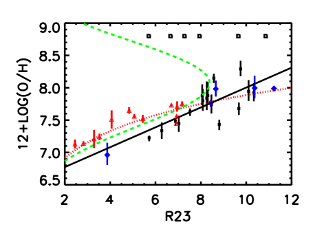
In Figure 10 we show the dependence of the present measurements of 12+log(O/H) on the R23 parameter. We also show the local points from Izotov and Thuan (2007) and the empirical fits of Yin et al. (2007) (red dotted curve) and Nagao et al. (2006) (green dashed curve). It is clear that the present data have lower 12+log(O/H) determinations at the same R23. This would be expected if the ionization parameters are higher in the present sample. A factor of five increase in the $q$ parameter could easily produce the offsets seen. Empirically we find a relation of the form 12+log(O/H)=6.45 + $0.15$ R23, which is shown as the black line in Figure 10, provides a reasonable description of the data.

Figure 10.— The oxygen abundance versus the R23 parameter for the [O III] selected sample (black squares) and the H$\alpha$ selected objects (blue diamonds). Galaxies with [O III]$\lambda$4363 lines below the two sigma level are shown with open squares at a nominal O abundance. One sigma errors are shown for the oxygen abundances. A linear fit to the combined data sets is shown by the black line while fits to the local data by Nagao et al. (2006) are shown with the green dashed line and by Yin et al. (2007) as the red dotted line. Local data from Izotov and Thuan (2007) are shown by the red triangles.

5.3. Metallicity versus H$\beta$ equivalent width

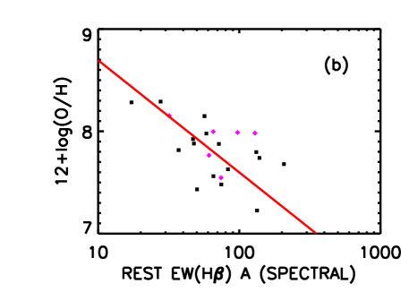
As is well known the H$\beta$ equivalent width can give a rough estimate of the age of the star formation in a galaxy. For a Salpeter IMF and a constant star formation rate, EW(H$\beta$) would drop smoothly to a value of 30Å at about $10^{9}$ yr (Leitherer et al., 1999) while an instantaneous starburst would drop below this value after about $10^{7}$ yr. It is therefore of considerable interest to determine the relation between 12+log(O/H) and EW(H$\beta$) in order to find if the metal build up is a function of the age of the galaxy.

We can determine EW(H$\beta$) in two ways. We can measure it directly from the spectra or we can determine the EW of the line falling in the narrow band filter from the imaging observations and then use the line ratios to determine EW(H$\beta$). However, both methods are somewhat problematic. Because the continuua in the spectra are extremely weak it can be difficult to precisely measure them. The errors here are complex and systemic efforts can be important. Thus EW(H$\beta$) can only be confidently measured in the highest S/N spectra. The imaging data makes a much deeper and more accurate measurement of the continuum but translating this to the observed frame EW of the measured line requires us to know the filter profile extremely accurately. This is a particular problem for objects whose wavelengths lie on the edges of the filter where the response changes rapidly. We measured EW(H$\beta$) with both methods. For the spectral determination we restricted ourselves to spectra with S/N$>25$ in the [O III]$\lambda$5007 line. For the images we restricted ourselves to galaxies where the transmission in the filter was above 80% of the peak transmission. We took the continuum from line free broad band colors near the narrow band (the $I$ band for the NB816 filter and the $z^{\prime}$ band for the NB912 filters) assuming that the spectrum $f_{\nu}$ was flat. We determined the EW of the line in the narrow band as ($10^{-0.4(N-C)}-1)/\phi$ where $N$ is the narrow band magnitude, $C$ is the continuum magnitude and $\phi$ is the filter response normalized such that the integral over the wavelength is unity. Where the line in the filter was [O III]$\lambda$5007 we converted to EW(H$\beta$) using the observed line ratios in the spectra and where the line in the filter was H$\alpha$ we converted to EW(H$\beta$) assuming the Case B Balmer ratios.

Figure 11.— Comparison of rest frame equivalent widths determined from the imaging data with those determined from the spectra. Black squares show [O III]$\lambda$5007 equivalent widths and purple diamonds H$\alpha$ equivalent widths. The red line shows the expected relation. Only objects where the line wavelength would correspond to a transmission above 80% of the peak filter response in the narrow band filter and where the [O III]$\lambda$5007 line is detected in the spectra at a signal to noise above 25 are shown.

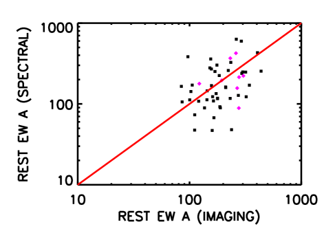
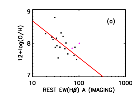
We compare the imaging equivalent widths with the spectroscopic equivalent widths in Figure 11. There is broad overall agreement but a considerable amount of scatter reflecting the uncertainties in the two methods. However, as is shown in Figure 12, irrespective of which method we use we see a clear relationship between 12+log(O/H) and EW(H$\beta$). The best fit relationship of 12+log(O/H) = $9.72-1.07$ log(EW(H$\beta$) based on the imaging equivalent widths also provides a good description for the spectroscopically based equivalent widths. This relation was less clear in the equivalent widths determined from the poorer spectra used in Kakazu et al. (2007). With the new data there is now clear evidence for the build-up of metals as a function of age in the galaxies.

5.4. Metallicity Luminosity relation

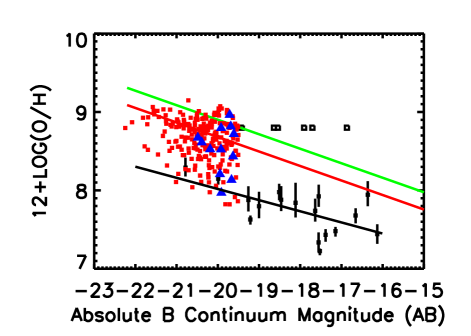
We next computed the absolute rest frame B magnitudes using magnitudes from imaging observations in bandpasses which are clear of the emission lines and assuming a flat $f_{\nu}$ spectral energy distribution to compute the K correction. We plot these absolute rest frame $B$ magnitudes versus the oxygen abundance derived by the direct method in Figure 13. The metallicity-luminosity relation can be written as 12+log(O/H) $=8.01-0.15\times(M_{B}(AB)-20)$.

We can compare the metallicity luminosity relation with the local metallicity luminosity relation from Tremonti et al. (2004) (the green line in Figure 13) and with observations of magnitude limited samples at $z=0.6-0.9$ from Cowie and Barger (2008) (red points) and the corresponding metal-luminosity relation at this redshift (red line). The present sample lies about 0.6 dex below the $z=0.6-0.9$ relation and about 0.8 dex lower than the local relation. The Cowie and Barger metallicities are based on the upper branch of the O versus R23 relation and may miss some low metallicity objects. We have also searched their magnitude limited sample for strong emitters (the blue diamonds in Figure 13) and checked these galaxies for [O III]$\lambda$4363 but none of these show the auroral line.

Figure 12.— (a) 12+log(O/H) versus rest frame H$\beta$ equivalent widths determined from the imaging data. Black squares show [O III]$\lambda$5007 selected objects and purple diamonds H$\alpha$ selected objects. The red line shows the best fit linear relation between 12+log(O/H) and log(EW(H$\beta$)). Only objects with filter transmission above 80% of the peak and with signal to noise above 15 for the H$\beta$ line are shown. (b) Same as (a) but with equivalent widths determined only from the spectra. All objects with signal to noise above 20 for the H$\beta$ line are shown. The red line is the fit to the imaging equivalent widths shown in (a).

Figure 13.— The oxygen abundance versus the absolute rest frame $B$ magnitude for the [O III] selected sample (black squares) The red diamonds show the oxygen abundances for a magnitude limited sample in the same redshift range from Cowie and Barger (2008). The green line shows the local metal-luminosity relation from Tremonti et al. (2004), the red the metallicity relation at $z=0.8$ from Cowie and Barger (2008), and the black line the metallicity-luminosity relation of the present sample.

6. Luminosity functions and the local Lyman alpha emitter population

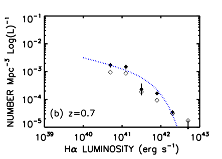
We next constructed the H$\alpha$ luminosity functions of the USEL sample following the procedures used in Kakazu et al. (2007) but using the present larger spectroscopic sample. We used the narrow band magnitudes to determine the line strength of the selection line; H$\alpha$ at low redshift and [O III]$\lambda$5007 at high redshift. For the higher redshift objects we computed the $H\beta$ flux from the [O III]$\lambda$5007 flux and converted this to an $H\alpha$ flux using the Case B ratio. Because of the high observed frame equivalent widths the primary fluxes are insensitive to the continuum determination. However, they do depend on the filter response at the emission line wavelength so we restricted ourselves to redshifts where the nominal filter response is greater than 80% of the peak value following the procedure used in the equivalent width analysis. This also has the advantage of providing a uniform selection and we assume the window function is flat over the defined redshift range. Now the volume is simply defined by the selected redshift range for all objects above the minimum luminosity which we take as corresponding to an observed flux of $1.5\times 10^{-17}$ erg cm^-2 s^-1 in the $H\alpha$ line. For the high redshift sample selected in the [O III]$\lambda$5007 line the true flux limit will generally be lower than this since the [O III]$\lambda$5007 line is normally stronger than H$\alpha$ and we restrict the sample to objects with $H\alpha$ line fluxes lying above this threshold. The luminosity function is now obtained by dividing the number of objects in each luminosity bin by the volume. The incompleteness corrected luminosity function is obtained from the sum of the weights in each luminosity bin divided by the volume. Here the weight of an object of a given magnitude correponds to the total number of objects at that magnitude divided by the number of identified ojects at that magnitude. Because of the high spectroscopic completeness the incompleteness corrections are small except at the very lowest luminosities. The 1 sigma errors shown are calculated from the Poissonian errors based on the number of spectroscopically identified objects in the bin. The calculated H$\alpha$ luminosity function is shown for the $z=0.2-0.45$ range corresponding to the NB816 and NB912 H$\alpha$ selections in Figure 14(a) and the corresponding H$\alpha$ luminosity function at $z=0.6-0.9$ from the [O III]$\lambda$5007 selected samples in Figure 14(b).

Figure 14.— The luminosity function of H$\alpha$ at $z=0.3$ (top panel a) and at $z=0.7$ (bottom panel b). In each case the open symbols show the luminosity functions determined from the spectroscopic sample alone while the solid symbols show the function corrected for the incompleteness in the spectroscopic identification. The errors are plus and minus 1 sigma and at the highest luminosity we show the 1 sigma upper limit. In panel (a) we also show the $z=0.3$ H$\alpha$ luminosity function from Tresse & Maddox (1998) as the blue dashed line. The dotted blue line shows the Tresse and Maddox function multiplied by 0.04 which approximately matches the USEL H$\alpha$ luminosity function. In panel (b) we show the Tresse and Maddox function multiplied by 0.18 which approximately matches the USEL H$\alpha$ luminosity function at the higher redshift.

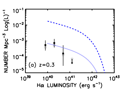
The USEL H$\alpha$ function at $z=0.3$ corresponds to about 4% of the total H$\alpha$ luminosity function at this redshift (Tresse & Maddox, 1998) which is shown as the blue dashed line in Figure 14(a). This is similar to the fraction of the total star formation rate that Kakazu et al. (2007) estimated was in the USELs. The USEL H$\alpha$ luminosity function rises rapidly with $z=0.3$ paralleling the rapid rise in the star formation rates over this redshift interval.

Figure 15.— The Ly$\alpha$ luminosity functions computed from the present samples assuming f(Ly$\alpha$)/f(H$\alpha$)$=5$ is shown at $z=0.3$ (black squares) and at $z=0.7$ (blue triangles). Only objects with rest frame equivalent widths above 20Å are included. The error bars are one sigma computed from the Poisson errors corresponding to the number of spectroscopically observed objects in the bin. We also show the one sigma upper limit (downward pointing arrow) at the highest luminosity. The Ly$\alpha$ luminosity function at the $z=0.3$ redshift derived from GALEX observations by Deharveng et al. (2008) is shown with the open red diamonds (actual obervations) and solid red diamonds (incompleteness corrected). It is clear that there are few local high luminosity LAEs in an area of the present size and there is no strong overlap between the present sample and the GALEX sample. We also show the $z=3$ LAE luminosity function of Gronwall et al. (2007) (solid red line) and the same function with a downward scaling of 4 (dashed red line) and 20 (dotted red line) in the number density.

These H$\alpha$ luminosity functions also allow us to construct upper limits on the $z=0-1$ Lyman alpha emitter luminosity functions for comparson with the local LAE luminosity function from GALEX (Deharveng et al., 2008) and with the measurements of the LAE luminosity function at high redshift ($z=2-7$). As we discuss in more detail below a galaxy with a high equivalent width in the Ly$\alpha$ line will also have a high equivalent width in H$\alpha$, so the LAEs are a subset of the present sample. This allows us to construct a upper bound on the complete LAE sample to a fixed Ly$\alpha$ equivalent width which can then be compared to the local and high redshift population in detail.

As is well known, the short path length to optical scattering on neutral hydrogen ensures that Lyman alpha photons follow a complex escape from a galaxy. While the low metallicity and extinction of the present USEL sample are clearly positive indicators of a higher Ly$\alpha$ escape fraction they are by no means the only factor. Internal structure, kinematics, and the distribution of star formation sites may also play key roles and may in fact be the more critical determinants. We take the Case B ratio of $8-12$ for the Ly$\alpha$/H$\alpha$ flux, depending on the electron density, to be an upper bound on the line ratio (Ferland and Osterbrock, 1985) (though we note that it is possible to have geometries in which the scattering can enhance the Ly$\alpha$ line relative to the UV continuum (Finkelstein et al., 2007).) Given the roughly flat $f_{\nu}$ continua in these galaxies (or $f_{\lambda}\sim\lambda^{-2}$), and the rest-frame fully complete to a rest equivalent-width of 30Å compared to the 20Å equivalent width normally used to select the high-redshift LAE population. The higher redshift $z\sim 0.7$ sample will contain all LAEs above 20Å for the case B assumption. However, empirical estimates of the Ly$\alpha$ escape fraction in the high redshift LAE population made by comparing star formation rates estimated from the UV continuum with those from the Ly$\alpha$ line suggest escape fractions of 30-50% (Gawiser et al., 2007; Gawiser, 2008). If this lower ratio is applicable for the ratio of the Ly$\alpha$/H$\alpha$ fluxes. then all LAEs will be included in the present samples, though objects close to the H$\alpha$ limiting equivalent width will fall from the LAE sample. The LAE sample is therefore a subset of the present sample and we can directly obtain an upper bound on the LAE luminosity function from the USEL H$\alpha$ luminosity function.

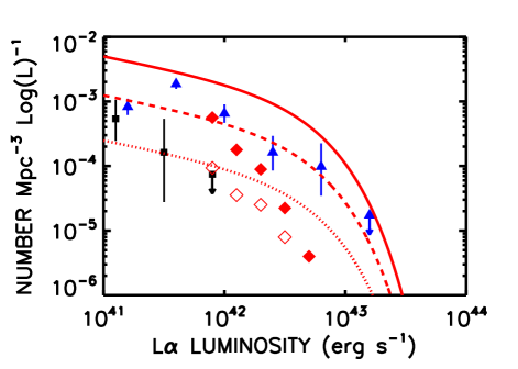
The sample is small but it provides a first-cut estimate of the evolution of the LAE luminosity function. We illustrate this in Figure 15 where we show the $z=0.3$ and the $z=0.7$ LAE luminosity functions that would be derived from our H$\alpha$ sample under the assumption Ly$\alpha$/H$\alpha$$=5$ for objects with rest frame Ly$\alpha$ equivalent widths above 20Å. The $z=0.3$ LAE luminosity function cam be compared with the direct determinations of the LAE luminosity function at this redshift from the GALEX observations of Deharveng et al. (2008) which are shown with the open red diamonds. The GALEX data only contain objects with strong UV continuum detections and these correspond to the highest luminosity emitters. In this sense they parallel the high redshift Lyman break galaxies with strong Lyman alpha emission rather than the line selected LAE samples. Deharveng et al. estimated that there should be a large incompleteness correction to allow for this selection effect and the solid red diamonds show their incompleteness corrected luminosity function. However, the present data, even under the case B assumption, suggest that the incompleteness corrections at the low luminosity end are smaller than the Deharveng et al. (2008) estimate. (We recall that the present data provide an absolute upper limit for the case B assumption.) The present $z=0.3$ sample has too small a volume to probe the high luminosity end.

At high redshifts the LAE luminosity function is surprisingly invariant in the range $z=2.5-6$ but there are signs it begins to drop at both higher and lower redshift. The present data show that it must have dropped substantially at redshift $z=0.7$ and even further at $z=0.3$. In Figure 15 we show the most recent determination of the $z=3$ LAE luminosity function from Gronwall et al. (2007). In order to match the present data the LAE luminosity function would have to drop by about a factor of four between $z=3$ and $z=0.7$ (dashed red line) and by a factor of very roughly twenty between $z=3$ and $z=0.3$ (dotted red line). Even under the case B assumption these drops would be two and ten respectively. The drop in the LAE luminosity fuction parallels the drop in the star formation over this redshift interval and there is even a suggestion of donwsizing in the shape of the LAE LF at the lowest redshift which is deficient in high luminosity objects relative to the low luminosity end.

7. Summary

We have described the results of deep spectroscopic observations of a narrow band selected sample of extreme emission line objects. The results show that such objects are common in the $z=0-1$ redshift interval and that a very large fraction of the strong emitters are detected in the [O III]$\lambda$4363 line where oxygen abundances can be measured using the direct method. The abundances primarily lie in the 12+log(O/H) range of 7$-$8 characteristic of XMPGs. We have determined the metal-luminosity relation for this class of object finding it lies about 0.6 dex below a magnitude selected sample in the same redshift interval. We give an emprical relation between R23 and 12 + log(O/H) which differs from local estimates. We also show that low metallicity objects can be picked out by the weakness of [O II]$\lambda$3727/[O III]$\lambda$5007 in the spectra. The two lowest metallicity galaxies in the sample have 12 + log(O/H) = $6.97\pm 0.17$ and $7.25\pm 0.03$, making them among the lowest metallicity galaxies known, but we expect that as the sample size is increased yet lower metallicity galaxies may be found and that we may hope to be able to determine if there is a floor in the galaxy metallicity at these redshifts.

References

- Cowie et al. (1996) Cowie, L. L., Songaila, A., Hu, E. M., & Cohen, J. G. 1996, AJ, 112, 839
- Cowie and Barger (2008) Cowie, L. L., & Barger, A. J. 2008, ApJ, 686, 72
- Deharveng et al. (2008) Deharveng, J-M. et al. 2008, ApJ, 680, 107
- Faber et al. (2003) Faber, S. M. et al. 2003, Proc. SPIE, 4841, 1657
- Ferland and Osterbrock (1985) Ferland, G.J., & Osterbrock, D. E. 1985, ApJ, 289, 105
- Finkelstein et al. (2007) Finkelstein, S. L., Rhoads, J. E., Malhotra, S., Pirzkal, N., & Wang, J. 2007, ApJ, 660, 1023
- Garnett (1992) Garnett, D. R. 1992, AJ, 103, 1330
- Gawiser et al. (2007) Gawiser, E. et al. 2007, ApJ, 671, 278
- Gawiser (2008) Gawiser, E. 2008, “LAEs are Similar to Other High-redshift Galaxies,” (review talk presented at Understanding Lyman Alpha Emitters Workshop, Heidelberg, MPIA, October 2008).
- Gronwall et al. (2007) Gronwall, C. et al. 2007, ApJ, 667, 79
- Izotov et al. (2005) Izotov, Y. I., Thuan, T. X., & Guseva, N. G., 2005, ApJ, 632, 210
- Izotov et al. (2006a) Izotov, Y. I., Papaderos, P., Guseva, N. G., Fricke, K. J., & Thuan, T. X. 2006a, A&A, 454, 137
- Izotov (2006b) Izotov, Y. I. 2006b, in ASP Conf. Ser. 353, Stellar Evolution at Low Metallicity: Mass Loss, Explosions, Cosmology, ed. H. J. G. L. M. Lamers, N. Langer, T. Nugis, & K. Annuk (San Francisco: ASP), 349
- Izotov et al. (2006c) Izotov, Y. I., Stasińska, G., Meynet, G., Guseva, N. G., & Thuan, T. X. 2006c, A&A, 448, 955
- Izotov and Thuan (2007) Izotov, Y. I., & Thuan, T. X. 2007, ApJ, 665, 1115
- Kakazu et al. (2007) Kakazu, Y., Hu, E. M., & Cowie, L. L. 2007 ApJ, 668, 853
- Kniazev et al. (2003) Kniazev, A. Y., Grebel, E. K., Hao, L., Strauss, M. A., Brinkmann, J., & Fukugita, M. 2003, ApJ, 593, L73
- Kobulnicky & Kewley (2004) Kobulnicky, H. A., & Kewley, L. J. 2004, ApJ, 617, 240
- Kunth & Östlin (2000) Kunth, D., & Östlin, G. 2000, A&A Rev., 10, 15
- Leitherer et al. (1999) Leitherer, C. et al. 1999, ApJS, 123, 3
- Nagao et al. (2006) Nagao, T., Maiolino, R., & Marconi, A. 2006, A&A, 459, 85
- Oey (2006) Oey, M. S. 2006, in ASP Conf. Ser. 353, Stellar Evolution at Low Metallicity: Mass Loss, Explosions, Cosmology, ed. H. J. G. L. M. Lamers, N. Langer, T. Nugis, & K. Annuk (San Francisco: ASP), 253
- McGaugh (1991) McGaugh, S. 1991, ApJ, 380, 140
- Pagel et al. (1979) Pagel, B.E.J., Edmunds, M. G., Blackwell, D. E., Chun, M. S., and Smith, G. 1979, MNRAS, 189, 95
- Pagel et al. (1992) Pagel, B.E.J., Simonson, E. A., Terlevich, R. J., & Edmunds, M. G. 1992, MNRAS, 255, 325
- Pilyugin (2000) Pilyugin, L. S., 2000, A&A, 362, 325
- Pilyugin & Thuan (2005) Pilyugin, L. S., & Thuan, T. X. 2005, ApJ, 631, 231
- Sargent & Searle (1970) Sargent, W. L. W., & Searle, L. 1970, ApJ, 162, L155
- Seaton (1975) Seaton M. J. 1975, MNRAS, 170, 475
- Tremonti et al. (2004) Tremonti, C. A, et al. 2004, ApJ, 613, 898
- Tresse & Maddox (1998) Tresse, L., and Maddox, S. J., 1998, ApJ, 495, 691
- Thuan & Izotov (2005) Thuan, T. X., Izotov, Y. I. 2005, ApJS, 161, 240
- Yin et al. (2007) Yin, S. Y., Liang, Y. C., Hammer, F., Brinchmann, J., Zhang, B., Deng, L. C., & Flores, H. 2007, A&A, 462, 535