Angle contraction between geodesics

Abstract

We consider here a generalization of a well known discrete dynamical system produced by the bisection of reflection angles that are constructed recursively between two lines in the Euclidean plane. It is shown that similar properties of such systems are observed when the plane is replaced by a regular surface in $\mathbb{R}^{3}$ and lines are replaced by geodesics. An application of our results to the classification of points on the surface as elliptic, hyperbolic or parabolic is also presented.

Keywords:
Geodesic triangles; Banach contraction principle; Gauss-Bonnet theorem
2000 Mathematics Subject Classification: 40A05; 53A05

1 Introduction

Let us consider the following simple problem. In the Euclidean plane take two rays starting at point $V$ and forming an acute angle of measure $\mu$. Denote the rays by $L_{A}$ and $L_{B}$ and take an arbitrary transversal segment $A_{1}B_{1}$ with $A_{1}\in L_{A}$, and $B_{1}\in L_{B}$. Keep constructing further segments with respect to the following rule: To create a new transversal, take the angle between the most recently constructed transversal and the corresponding ray, and let the new transversal be the bisector of this angle. In particular, if we have as our last transversal $B_{k-1}A_{k}$, we take the bisector of $\angle B_{k-1}A_{k}V$, denote its intersection with line $L_{B}$ by $B_{k}$ and use the transversal $A_{k}B_{k}$ for the next step (see Figure 1). Clearly, this process creates not only two sequences of points $\{A_{k}\}\in L_{A}$, $\{B_{k}\}\in L_{B}$ but also two sequences of angles $\{\alpha_{k}\}$, and $\{\beta_{k}\}$, where $\alpha_{k}=\angle B_{k}A_{k}V$, and $\beta_{k}=\angle A_{k+1}B_{k}V$.

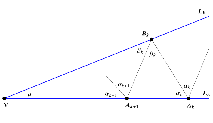
Figure 1:

By expressing each sequence of angles as a first order difference equation, it is easy to show that

$$\lim_{k\to\infty}\alpha_{k}=\lim_{k\to\infty}\beta_{k}=\frac{\pi-\mu}{3}$$

irrespective of the choice of the initial transversal segment. We show below that this property holds under more general circumstances. Specifically, we replace the plane with a smooth surface in $\mathbb{R}^{3}$, where our triangles will be geodesic triangles, and drop the condition that the angles are created by bisection.

2 A generalization of the problem

Let $S\subset\mathbb{R}^{3}$ be a regular surface locally parametrized by a differentiable vector function ${\bf r}(u,v):U\longrightarrow\mathbb{R}^{3}$, with $U$ being open in $\mathbb{R}^{2}$. All curves we consider below will be regular parametrized curves, that is, differentiable vector functions ${\bf c}:[a,b]\longrightarrow\mathbb{R}^{3}$ with $\dot{\bf c}(t)={\rm d}{\bf c}(t)/{\rm d}t\neq 0$ for all values of the parameter $t\in(a,b)$. By a geodesic on $S$ we will mean a unit speed regular curve ${\bf c}(s)$ (parametrized by the arc length) on $S$ such that the second derivative ${\bf c}^{\prime\prime}(s)$ is the zero vector or perpendicular to the surface.

To avoid the cases when two distinct points on $S$ can be joined by different geodesics, we will consider only “small” triangles formed by two geodesics intersecting at a point $V$ and a third geodesic intersecting the first two transversally at points $A$ and $B$. By a “small” triangle we will mean one contained in an open subset of $S$, which is a normal neighborhood of all its points. Proof of the existence of such a neighborhood for each point $p\in S$ can be found in §4-7 of [1].

If $\gamma_{v}:[0,b]\longrightarrow S,\gamma_{v}(0)=P,\gamma_{v}^{\prime}(0)=v$ and $\gamma_{w}:[0,c]\longrightarrow S,\gamma_{w}(0)=P$, $\gamma_{w}^{\prime}(0)=w$ are two geodesics at $P$, the angle between these two geodesics is defined to be the angle between $v$ and $w$. If $X$ is on $\gamma_{v}$ and $Y$ is on $\gamma_{w}$, we will denote this angle either by $\angle XPY$ or by $\angle YPX$. Assume now that we are given a “small” triangle $\bigtriangleup VAB$ on a regular surface $S\subset\mathbb{R}^{3}$ and denote $\angle BVA$ by $\mu$, and assume that $\mu<\pi$.

As was the case in the Euclidean plane, we can construct first order difference equations for the angles created by bisection, where now our transversals will be geodesic segments. Let $A_{1}=A,~{}B_{1}=B$ and $\alpha_{1}:=\angle VA_{1}B_{1}$. Assume also that we are given two continuous functions $p:S\to\mathbb{R}^{+}$ and $q:S\to\mathbb{R}^{+}$ taking only positive values. To construct the point $A_{2}$ on the geodesic segment $VA_{1}$, we consider the geodesic $\gamma_{\beta_{1}}:[0,1]\to S$ such that $\gamma_{\beta_{1}}(0)=B_{1}$ and the angle between $\gamma^{\prime}_{\beta_{1}}(0)\in T_{B_{1}}(S)$ and the geodesic segment $B_{1}A_{1}$ is

$$\beta_{1}=\frac{\angle VB_{1}A_{1}}{1+q(B_{1})}.$$

Geodesic $\gamma_{\beta_{1}}([0,a))$ (with $a$ large enough) will intersect transversally the segment $VA_{1}$ at a point, which we denote by $A_{2}$. Then we use function $p:S\to\mathbb{R}^{+}$ and divide angle $\angle B_{1}A_{2}V$ by the geodesic $\gamma_{\alpha_{2}}:[0,1]\to S$ to create the point $B_{2}$ on segment $VB_{1}$, where $\gamma_{\alpha_{2}}(0)=A_{2}$ and the angle between $\gamma^{\prime}_{\alpha_{2}}(0)\in T_{A_{2}}(S)$ and segment $A_{2}V$ is defined by

$$\alpha_{2}=\frac{\angle VA_{2}B_{1}}{1+p(A_{2})}.$$

Point $B_{2}$ is defined as the intersection of $VB_{1}$ with geodesic $\gamma_{\alpha_{2}}([0,a))$ (see Figure 2, where we abbreviated $p(A_{m})$ and $q(B_{n})$ as $p_{m}$ and $q_{n}$ respectively).

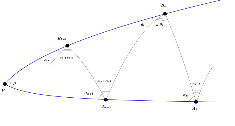
Figure 2:

Then we iterate this procedure to construct two sequences of points $\{A_{k}\}_{k=1}$, $\{B_{k}\}_{k=1}$, and angles

$$\alpha_{k+1}=\frac{\angle VA_{k+1}B_{k}}{1+p(A_{k+1})},~{}~{}~{}~{}~{}{\rm and}~{}~{}~{}~{}~{}\beta_{k}=\frac{\angle VB_{k}A_{k}}{1+q(B_{k})}$$

Here arises a natural question. Do the sequences $\{\alpha_{n}\}$ and $\{\beta_{n}\}$ converge, and if so, to what values? In the next section we will prove the following

Theorem 1.

For an arbitrary small triangle $\bigtriangleup VAB$ on a regular surface $S$ in $\mathbb{R}^{3}$ with the angle $\angle AVB=\mu<\pi$ and two continuous positive functions $p:S\longrightarrow\mathbb{R}^{+}$ and $q:S\longrightarrow\mathbb{R}^{+}$, we have

$$\lim_{n\to\infty}\alpha_{n}=\frac{q(V)\cdot(\pi-\mu)}{p(V)+q(V)+p(V)\cdot q(V)}$$

and

$$\lim_{n\to\infty}\beta_{n}=\frac{p(V)\cdot(\pi-\mu)}{p(V)+q(V)+p(V)\cdot q(V)}$$

Corollary 1.

If, in addition to the conditions of the theorem we assume that functions $p$ and $q$ are equal, then

$$\lim_{n\to\infty}\alpha_{n}=\lim_{n\to\infty}\beta_{n}=\frac{\pi-\mu}{2+p(V)}$$

Recall that a point $x\in S$ is called elliptic when the Gauss curvature $K(x)>0$, hyperbolic when $K(x)<0$ and parabolic when $K(x)=0$. Our next corollary shows that there exist functions $p(x)$ and $q(x)$ so that the limits of our sequences of angles will distinguish the type of the point $V$.

Corollary 2.

Let $k_{1}(x)$ and $k_{2}(x)$ denote two principal curvatures at $x\in S$. If

$$p(x)=1+|K(x)\cdot(k_{1}(x)+k_{2}(x))|~{}~{}~{}{\rm and}~{}~{}~{}q(x)=1+|K(x)|\cdot(|k_{1}(x)|+|k_{2}(x)|)$$

then the pairs $(\lim\alpha_{n},~{}\lim\beta_{n})$ are different for different type of points.

Proof.

Straightforward computations show that in the case of a parabolic, elliptic, and hyperbolic points correspondingly, we have

$$~{}~{}\lim\alpha_{n}=\lim\beta_{n}=\frac{\pi-\mu}{3},~{}~{}\lim\alpha_{n}=\lim\beta_{n}<\frac{\pi-\mu}{3},~{}~{}\lim\alpha_{n}\neq\lim\beta_{n}.$$

∎

3 Proof of the theorem

The proof of Theorem 1 relies on a generalization of the Banach contraction mapping principle and a special case of the local version of the Gauss-Bonnet Theorem. Let us first recall the contraction principle.

The Contraction Theorem Consider a complete metric space $(M,{\rm dist})$. Let $T:M\to M$ be a contraction mapping with Lipschitz constant $k\in(0,1)$, and suppose $\alpha\in M$ is the fixed point of $T$. Let $\{\varepsilon_{n}\}$ be a sequence of positive numbers converging to zero, and suppose $\{\alpha_{n}\}\subseteq M$ satisfies:

$${\rm dist}(\alpha_{n+1},~{}T(\alpha_{n}))\leq\varepsilon_{n}.$$

Then the sequence $\{\alpha_{n}\}$ converges to $\alpha$. We refer the reader to chapter 3 of [2] for a proof of this theorem.

Proof of Theorem 1.

Let’s apply the Gauss-Bonnet Theorem to geodesic triangles $A_{k}B_{k}A_{k+1}$ and $A_{k}B_{k}V$. Using notations from figure 2, one will get the following:

$$\iint\limits_{A_{k}B_{k}A_{k+1}}K~{}dS=\alpha_{k}+q(B_{k})\cdot\beta_{k}+(\pi-(1+p(A_{k+1}))\cdot\alpha_{k+1})-\pi,$$

which is equivalent to the formula

$$\alpha_{k+1}=\frac{\alpha_{k}}{1+p(A_{k+1})}+\frac{q(B_{k})\cdot\beta_{k}}{1+p(A_{k+1})}-\frac{1}{1+p(A_{k+1})}\cdot\iint\limits_{A_{k}B_{k}A_{k+1}}K~{}dS,$$ (1)

and similarly

$$\iint\limits_{A_{k}B_{k}V}K~{}dS=\alpha_{k}+(1+q(B_{k}))\cdot\beta_{k}+\mu-\pi,$$

which gives $\beta$ in terms of $\alpha$ and $\mu$:

$$\beta_{k}=\frac{\pi-\mu}{1+q(B_{k})}-\frac{\alpha_{k}}{1+q(B_{k})}+\frac{1}{1+q(B_{k})}\cdot\iint\limits_{A_{k}B_{k}V}K~{}dS.$$ (2)

Substituting (2) into (1) one easily obtains

$\alpha_{k+1}=\\ ~{}\\ \frac{\alpha_{k}+q(B_{k})\cdot(\pi-\mu)}{(1+p(A_{k+1}))\cdot(1+q(B_{k}))}+\frac{q(B_{k})}{(1+p(A_{k+1}))\cdot(1+q(B_{k}))}\cdot\iint\limits_{A_{k}B_{k}V}K~{}dS-\frac{1}{1+p(A_{k+1})}\cdot\iint\limits_{A_{k}B_{k}A_{k+1}}K~{}dS$

Since $p(X)>0$ and $q(X)>0$ for an arbitrary point $X\in S$, the map

$$T(\varphi):=\frac{1}{(1+p(V))\cdot(1+q(V))}\cdot\varphi+\frac{q(V)\cdot(\pi-\mu)}{(1+p(V))\cdot(1+q(V))}$$

will be a contraction with Lipschitz constant $1/[(1+p(V))\cdot(1+q(V))]\in(0,1)$. Its fixed point $\alpha$ can be found by a straight forward computation

$$\alpha=\frac{q(V)\cdot(\pi-\mu)}{p(V)+q(V)+p(V)\cdot q(V)}.$$

To apply the contraction theorem for this map $T$, we set $M=\mathbb{R}$ with the standard distance function ${\rm dist}(x,y):=|x-y|$. Then it follows that
 
$\varepsilon_{k}:=|\alpha_{k+1}-T(\alpha_{k})|=|\frac{\alpha_{k}+q(B_{k})\cdot(\pi-\mu)}{(1+p(A_{k+1}))\cdot(1+q(B_{k}))}-T(\alpha_{k})+\frac{q(B_{k})}{(1+p(A_{k+1}))\cdot(1+q(B_{k}))}\cdot\iint\limits_{A_{k}B_{k}V}KdS-\\ \frac{1}{1+p(A_{k+1})}\cdot\iint\limits_{A_{k}B_{k}A_{k+1}}KdS~{}|$

Thus, to prove our theorem for the sequence $\{\alpha_{n}\}$, it is enough to show that $\{\varepsilon_{k}\}\to 0$ when $k\to\infty$. For this we will show that the difference of two fractions and each of the double integrals in the formula for $\varepsilon_{k}$ converge to zero. The Gaussian curvature of a regular surface is a smooth function, and hence it is universally bounded on a small triangle. Since the union of all triangles $\bigtriangleup A_{k}B_{k}A_{k+1}$ is contained in the small triangle $\bigtriangleup VAB$, we must have

$$\sum\limits_{k=1}^{\infty}~{}\iint\limits_{A_{k}B_{k}A_{k+1}}\left|K\right|~{}dS<\iint\limits_{ABV}\left|K\right|~{}dS<\infty,$$

and hence the general term of the series converges to zero. As for the integrals over the triangles $A_{k}B_{k}V$, we first notice that both sequences $\{A_{k}\}$ and $\{B_{k}\}$ converge to the vertex $V$ (see Lemma 1 below). Therefore length of each of three geodesics $L(A_{k},V)$, $L(B_{k},V)$ and $L(A_{k},B_{k})$ approaches zero, which implies that the regions in $\mathbb{R}^{2}$ corresponding to the triangles $\bigtriangleup A_{k}B_{k}V$ get shrunk to a point. Hence

$$\iint\limits_{A_{k}B_{k}V}K~{}dS\stackrel{{\scriptstyle k\to\infty}}{{\longrightarrow}}0.$$

Convergence to zero of

$$\frac{\alpha_{k}+q(B_{k})\cdot(\pi-\mu)}{(1+p(A_{k+1}))\cdot(1+q(B_{k}))}-T(\alpha_{k})$$

follows from the lemma since both functions $p,q:S\longrightarrow\mathbb{R}^{+}$ are continuous. Thus, $\varepsilon_{k}\longrightarrow 0$, when $k\to\infty$, and hence our result for $\{\alpha_{k}\}$. To finish the proof take the limit as $k\to\infty$ of each side in formula (2) to obtain the desired answer for the sequence $\{\beta_{k}\}$. ∎

Lemma 1.

$\lim\limits_{k\to\infty}B_{k}=\lim\limits_{k\to\infty}A_{k}=V$

Proof.

Suppose we are given a geodesic segment $PQ\subset S$. As above, we will designate here the length of such a segment by $L(P,Q)$. Since our triangle $\bigtriangleup B_{1}VA_{1}$ is a small one, it is easy to see that the sequence of points $\{B_{k}\}$ converges to a point, $P$, on the geodesic segment $B_{1}V$. Assume that $P\not=V$. Then $\forall\varepsilon>0$, sufficiently small, $~{}\exists N$, a large enough natural number, such that $\forall k\geq N$, $B_{k}$ will be in a neighborhood of radius $\varepsilon$ centered at $P$ and contained in $exp_{p}(D_{\varepsilon})$. Further, we assume that $\varepsilon$ is so small that $exp_{p}(D_{\varepsilon})$ has no points in common with the segment $A_{1}V$. This implies that $\exists c>0$ such that for all large enough $n,~{}m$ we also have $L(A_{n},B_{m})>c$. Consider a regular parametrization $\gamma(t):~{}[0,\theta]\longrightarrow B_{1}V$ of the geodesic $B_{1}V$ such that $\gamma(0)=B_{1}$, $\gamma(\theta)=V$ and ${\rm d}\gamma(t)/{\rm d}t\neq 0,~{}\forall t\in(0,\theta).$ Let us denote by $t_{k}\in[0,\theta]$, $t_{1}=0$, the parameter value corresponding to the point $B_{k}\in B_{1}V$, i.e. $\gamma(t_{k})=B_{k}$. Since the sequence $\{B_{k}\}$ converges and $\gamma(t)$ is smooth, the corresponding sequence of parameters $\{t_{k}\}$ will converge as well.

As the next step, we use the exponential map to show that existence of the limit point $P$ with $L(P,V)>0$ implies the convergence to zero of both sequences $\{\alpha_{k}\}$ and $\{\beta_{k}\}$. Assume that $n$ is large enough and recall that $exp_{A_{n}}:~{}T_{A_{n}}S\longrightarrow S$ is a diffeomorphism locally and its image contains our small triangle $\bigtriangleup ABV$. In particular, we can consider the preimage of the two geodesics segments $B_{n}A_{n}$, and $A_{n}B_{n+1}$, which will be line segments in $T_{A_{n}}S$. We denote those lines by $(\tilde{B}_{n}A_{n})$ and $(A_{n}\tilde{B}_{n+1})$ respectively(i.e. $exp^{-1}_{A_{n}}(B_{n})=\tilde{B}_{n}$). Since $exp_{A_{k}}$ preserves the angles and lengths of rays through the point $A_{k}$, we have that

$$\angle\tilde{B}_{n}A_{n}\tilde{B}_{n+1}=\angle B_{n}A_{n}B_{n+1}=p(A_{n})\cdot\alpha_{n}~{}~{}~{}{\rm and}~{}~{}~{}|A_{n}\tilde{B}_{n+i}|=L(A_{n},B_{n+i})>c,$$

where $i\in\{0,1\}$. We also have the following inequalities:

$$L(\tilde{B}_{n+1},\tilde{B}_{n})\geq{\rm dist}[\tilde{B}_{n+1},(A_{n}\tilde{B}_{n})]>c\cdot{\rm sin}(p(A_{n})\cdot\alpha_{n}),$$

where $L(\tilde{B}_{n+1},\tilde{B}_{n})$ denotes the length of the curve $exp^{-1}_{A_{n}}[(B_{n+1}B_{n})]\subset T_{A_{n}}S$ and can be computed by the integral

$$L(\tilde{B}_{n+1},\tilde{B}_{n})=\int\limits^{t_{n+1}}_{t_{n}}|(exp^{-1}_{A_{n}}\circ\gamma)^{\prime}(u)|~{}du.$$

Since the composition $exp^{-1}_{A_{n}}\circ\gamma(t)$ is smooth, there exists a positive constant $K$ such that for all large enough $n$, we have

$$K\cdot|t_{n+1}-t_{n}|\geq L(\tilde{B}_{n+1},\tilde{B}_{n})>c\cdot{\rm sin}(p(A_{n})\cdot\alpha_{n}),$$

which implies that the sequence of angles $\{\alpha_{n}\}$ converges to zero. Recalling (2) we conclude that the sequence $\{\beta_{n}\}$ converges to zero as well.

Now let’s look at the triangle $\bigtriangleup A_{k}B_{k}V$ and consider the geodesic through $A_{k}$ and a point $Z$ on the geodesic segment $VB_{k}$, including both end points. Since $Z$ belongs to a closed and bounded curve, there is such geodesic $A_{k}Z$ of maximal length. Let’s denote this length by $L_{k}$, that is

$$L_{k}:=\max\limits_{Z\in B_{k}V}\left\{L(A_{k},Z)\right\}.$$

Now we take the circular sector of radius $L_{k}$, denoted by $\bigtriangleup S(A_{k},L_{k})$, centered at $A_{k}$ and bounded between two geodesics $A_{k}V$ and $A_{k}B_{k}$ with angle $\alpha_{k}$ at $A_{k}$. Clearly, $\bigtriangleup A_{k}B_{k}V\subset\bigtriangleup S(A_{k},L_{k})$, and therefore

$$\iint\limits_{A_{k}B_{k}V}\left|K\right|~{}dS\leq\iint\limits_{\bigtriangleup S(A_{k},L_{k})}\left|K\right|~{}dS.$$

Since the sequence $\{L_{k}\}$ is certainly bounded and $\{\alpha_{k}\}\longrightarrow 0$, when $k\to\infty$, the areas of $\bigtriangleup S(A_{k},L_{k})$ will approach zero, which implies that

$$\iint\limits_{A_{k}B_{k}V}K~{}dS\stackrel{{\scriptstyle k\to\infty}}{{\longrightarrow}}0.$$

Now one can use formula (2) to deduce that $\mu=\pi$, which will contradict the assumption that $\mu<\pi$ in the triangle $\bigtriangleup ABV$. A similar argument for $\{A_{k}\}$ also results in a contradiction. ∎

Siena College, School of Science
515 Loudon Road, Loudonville NY 12211

nkrylov@siena.edu and rogers@siena.edu

References

• [1] Manfredo P. do Carmo:Β Differential geometry of curves and surfaces, Prentice-Hall, Inc., Englewood Cliffs, N.J., 1976.
• [2] Mohamed A. Khamsi, William A. Kirk:Β An introduction to metric spaces and fixed point theory, Wiley-Interscience Publication, John Wiley & Sons, Inc., New York, 2001.