Fluctuation conductivity from interband pairing in pnictides

Abstract

We derive the effective action for superconducting fluctuations in a four-band model for pnictides, discussing the emergence of a single critical mode out of a dominant interband pairing mechanism. We then apply our model to calculate the paraconductivity in two-dimensional and layered three-dimensional systems, and compare our results with recent resistivity measurements in SmFeAsO_0.8F_0.2.

The recent discovery of superconductivity in pnictides kamihara has renewed the interest in high-temperature superconductivity. Pnictides share many similarities with cuprate superconductors, e.g., the layered structure, the proximity to a magnetic phase uemura , the relatively large ratio between the superconducting (SC) gap and the critical temperature $T_{c}$ ding ; gonnelli , and the small superfluid density uemura . However, differently from cuprates, the presence of several sheets of the Fermi surface makes the multiband character of superconductivity an unavoidable ingredient of any theoretical model for pnictides. Moreover, since the calculated electron-phonon coupling cannot account for the high values of $T_{c}$ boeri ; mazin , it has been suggested that the pairing glue is provided by spin fluctuations exchanged between electrons in different bands mazin ; spin_fluc ; chubukov . Thus, pnictides are expected to be somehow different from other multiband superconductors (e.g., MgB₂) where the main coupling mechanism is intraband liu .

This scenario raises interesting questions regarding the appropriate description of SC fluctuations in a multiband system dominated by interband pairing. The issue is relevant, because fluctuating Cooper pairs above $T_{c}$ contribute to several observable quantities, such as, e.g., the enhancement of dc conductivity (paraconductivity) and of the diamagnetic response as $T_{c}$ is approached LV . The nature of SC fluctuations depends on whether the system is weakly or strongly coupled (and on whether preformed pairs are present or not) and a wealth of physical information can be obtained from paraconductivity and diamagnetic response, provided a theoretical background is established to extract them.

In this paper, after introducing a four-band model, as appropriate for pnictides, we discuss the subtleties related to the description of SC fluctuations in a system with dominant interband pairing. We then apply our results to compute the paraconductivity associated with SC fluctuations above $T_{c}$. We show that when interband pairing dominates, despite the presence of four bands, there are only two independent fluctuating modes. Only one of them is critical and yields a diverging Aslamazov-Larkin (AL) contribution to paraconductivity as $T_{c}$ is approached, similarly to the case of dominant intraband pairing varlamov . The temperature dependence of the AL paraconductivity is the same derived for ordinary single-band superconductors al ; LV . Remarkably, within a BCS approach, we recover the AL numerical prefactor, which is a universal coefficient in two dimensions, and depends instead on the coherence length perpendicular to the planes in the three-dimensional layered case. We also find that subleading terms with respect to the leading AL contribution could distinguish between dominant inter- and intra-band pairing. Within this theoretical background, we analyze recent resistivity data in SmFeAsOF gonnelli and discuss the results.

At present, ARPES measurements in pnictides ding confirmed the Fermi-surface topology predicted by LDA. It consists of two hole-like pockets centered around the $\Gamma$ point (labeled $\alpha$ and $\beta$, following Ref. [ding, ]), and two electron-like ($\gamma$) pockets centered around the M points of the folded Brillouin zone of the FeAs planes. Motivated by the magnetic character of the undoped parent compound and by the approximate nesting of the hole and the electron pockets with respect to the magnetic ordering wavevector, we assume that pairing mediated by spin fluctuations is effective only between hole and electron bands chubukov . Since the $\beta$ band has a Fermi surface substantially larger than the $\alpha$ band, the $\beta$ pocket is expected to be less nested to the $\gamma$ pocket, so that the interband $\beta-\gamma$ coupling $\lambda$ is smaller than the $\alpha-\gamma$ coupling $\L$, i.e., $\eta\equiv\lambda/\Lambda<1$. The two electron pockets have comparable sizes and for simplicity we assume that the $\gamma$ bands are degenerate. Therefore, the BCS Hamiltonian of our four-band model is benfatto_4bands

$$H=\sum_{i}H_{0}^{i}+\Lambda\sum_{\bf q}\left[\Phi^{\dagger}_{\gamma,{\bf q}}(\Phi^{\phantom{\dagger}}_{\alpha,{\bf q}}+\eta\Phi^{\phantom{\dagger}}_{\beta,{\bf q}})+h.c.\right],$$ (1)

where $H_{0}^{i}=\sum_{\bf k}\xi_{i,{\bf k}}c^{\dagger}_{i,{\bf k}\sigma}c^{\phantom{\dagger}}_{i,{\bf k}\sigma}$ is the band Hamiltonian, $c_{i,{\bf k}\sigma}^{(+)}$ annihilates (creates) a fermion in the $i=\alpha,\beta,\gamma_{1},\gamma_{2}$ band (with the twofold degenerate $\gamma$ bands labeled as $\gamma_{1}$ and $\gamma_{2}$), $\xi_{i,{\bf k}}$ is the dispersion with respect to the chemical potential, $\Phi_{i,{\bf q}}=\sum_{\bf k}c^{\phantom{\dagger}}_{i,{\bf k}+{\bf q}\uparrow}c^{\phantom{\dagger}}_{i,{\bf k}\downarrow}$ is the pairing operator in the $i$-th band, and $\Phi_{\gamma,{\bf q}}\equiv\Phi_{\gamma_{1},{\bf q}}+\Phi_{\gamma_{2},{\bf q}}$. Since we assumed that pairing acts between hole and electron bands only, we can express the pairing term in Eq. 1 by means of $\Phi_{1}\equiv\Phi_{\gamma}$ and $\Phi_{2}\equiv\Phi_{\alpha}+\eta\Phi_{\beta}$. Thus

$$H_{I}=\Lambda\sum_{\bf q}(\Phi_{1}^{\dagger}\Phi_{2}^{\phantom{\dagger}}+h.c.)=-\Lambda\sum_{\bf q}(\Phi_{-}^{\dagger}\Phi^{\phantom{\dagger}}_{-}-\Phi_{+}^{\dagger}\Phi^{\phantom{\dagger}}_{+}),$$ (2)

where $\Phi_{\pm}=(w_{1}\Phi_{1}\pm w_{2}\Phi_{2})/\sqrt{2}$, $w_{1},w_{2}$ are arbitrary numbers satisfying $w_{1}w_{2}=1$, and for definiteness we take $\Lambda>0$, which is the case for a spin-mediated pairing interaction. From Eq. (2) one immediately sees that when interband pairing dominates, the interaction is a mixture of attraction (for $\Phi_{-}$) and repulsion (for $\Phi_{+}$). As a consequence, when we perform the standard Hubbard-Stratonovich (HS) decoupling of the quartic interaction term (2) by means of the HS field $\phi$,

$$e^{\pm\Lambda\Phi^{\dagger}\Phi} = \int{\cal{D}}\phi\,e^{-|\phi|^{2}/\Lambda+\sqrt{\pm 1}(\Phi^{\dagger}\phi+h.c.)},$$ (3)

the HS transformation associated with the repulsive part contains the imaginary unit. As we shall see below, this would require an imaginary value of the $\phi_{+}$ HS field at the saddle point, that can be avoided by the rotation of the pairing operators $\Phi_{\pm}$ defined above, via a suitable choice of the $w_{1,2}$ coefficients.

In analogy with the single-band case lara_pp , the effective action for the SC fluctuations reads

$$S = \sum_{i}\sum_{k}\sum_{\sigma}(\xi_{i,{\bf k}}-i\varepsilon_{n})c^{\dagger}_{i,k\sigma}c^{\phantom{\dagger}}_{i,k\sigma}$$

$$+ \sum_{q}\left[\frac{|\phi_{+}(q)|^{2}}{\Lambda}-i\phi_{+}^{*}(q)\Phi^{\phantom{\dagger}}_{+}(q)-i\phi_{+}(q)\Phi^{\dagger}_{+}(q)\right]$$

$$+ \sum_{q}\left[\frac{|\phi_{-}(q)|^{2}}{\Lambda}-\phi_{-}^{*}(q)\Phi^{\phantom{\dagger}}_{-}(q)-\phi_{-}(q)\Phi^{\dagger}_{-}(q)\right],~{}~{}~{}~{}$$

where $k\equiv({\bf k},i\varepsilon_{n})$, $q\equiv({\bf q},i\omega_{m})$, and $\varepsilon_{n}$, $\omega_{m}$ are the Matsubara fermion and boson frequencies, respectively. Integrating out the fermions we obtain the standard contribution to the action, $-\sum_{i}{\mathrm{Tr}}\log A^{i}_{kk^{\prime}}$, where the trace acts on momenta, frequencies, and spins. The elements of the matrices $A^{i}_{kk^{\prime}}$ are

$$\left[A^{i}_{kk^{\prime}}\right]_{11}=(\xi_{i,{\bf k}}-i\varepsilon_{n})\delta_{kk^{\prime}},~{}~{}~{}\left[A^{i}_{kk^{\prime}}\right]_{22}=-(\xi_{i,{\bf k}}+i\varepsilon_{n})\delta_{kk^{\prime}},$$

with $i=\alpha,\beta,\gamma_{1},\gamma_{2}$,

$$\left[A^{\alpha\phantom{\beta}}_{kk^{\prime}}\right]_{12} = \frac{w_{2}}{\sqrt{2}}\left[{\phi_{-}(k-k^{\prime})-i\phi_{+}(k-k^{\prime})}\right],$$

$$\left[A^{\beta}_{kk^{\prime}}\right]_{12} = \eta\left[A^{\alpha\phantom{\beta}}_{kk^{\prime}}\right]_{12},$$

$$\left[A^{\gamma\phantom{\beta}}_{kk^{\prime}}\right]_{12} = -\frac{w_{1}}{\sqrt{2}}\left[{\phi_{-}(k-k^{\prime})+i\phi_{+}(k-k^{\prime})}\right],$$

for $\gamma=\gamma_{1},\gamma_{2}$, and the $[A^{i}_{kk^{\prime}}]_{21}$ elements contain the complex conjugates of the HS fields evaluated at $(k^{\prime}-k)$.

The $q=k-k^{\prime}=0$ values of the HS fields yield the SC gaps in the various bands, within the saddle-point approximation $\phi_{\pm}(q=0)=\bar{\phi}_{\pm}$. However, due to the presence of the imaginary unit $i$ associated with the HS field $\phi_{+}$, in general $[A^{i}_{kk}]^{*}_{21}\neq[A^{i}_{kk}]_{12}$. To recover a Hermitian $A$ matrix at the saddle point, the integration contour of the functional integral must be deformed toward the imaginary axis of the $\phi_{+}$ field. This can be avoided if one chooses $w_{1}$ and $w_{2}$ in the definition of $\Phi_{\pm}$ in such a way that $\bar{\phi}_{+}=0$. In our case, the choice $\bar{\phi}_{+}=0$ gives $\Delta_{\alpha}=-w_{2}\bar{\phi}_{-}/\sqrt{2}$, $\Delta_{\gamma}=w_{1}\bar{\phi}_{-}/\sqrt{2}$ and $\Delta_{\beta}=\eta\Delta_{\alpha}$. Hence, the ratio of the gaps in the two hole bands is solely determined by the ratio of the couplings, $\Delta_{\beta}/\Delta_{\alpha}=\eta$. Using $w_{1}w_{2}=1$ we have $\bar{\phi}_{-}^{2}=-2\Delta_{\alpha}\Delta_{\gamma}$, and the equations for $\Delta_{\alpha}$ and $\Delta_{\gamma}$ read benfatto_4bands

$$\Delta_{\alpha} = -\Lambda(2\Pi_{\gamma})\Delta_{\gamma},$$ (4)

$$\Delta_{\gamma} = -\Lambda\left(\Pi_{\alpha}\Delta_{\alpha}+\eta\Pi_{\beta}\Delta_{\beta}\right),$$ (5)

where $\Pi_{i}=N_{i}\int_{0}^{\omega_{0}}d\xi[\tanh({E_{i}}/{2T})]/E_{i}$ yields the $q=0$ value of particle-particle bubble when $T>T_{c}$, $N_{i}$ is density of states of the $i$-th band at the Fermi level, $\omega_{0}$ is the cut-off for the pairing interaction, and $E_{i}=\sqrt{\xi^{2}+\Delta_{i}^{2}}$. Hence, our four-band model for pnictides effectively reduces to a two-band model, with one electron-like and one hole-like effective band. Indeed, defining $\Delta_{1}\equiv\Delta_{\gamma}$, $\Delta_{2}\equiv\Delta_{\alpha}$, and $\Pi_{1}\equiv 2\Pi_{\gamma}$, $\Pi_{2}\equiv\Pi_{\alpha}+\eta^{2}\Pi_{\beta}$, Eqs. (4)-(5) recover the standard two-band expression $\Delta_{1}=-\Lambda\Pi_{2}\Delta_{2}$ and $\Delta_{2}=-\Lambda\Pi_{1}\Delta_{1}$. Since $\Delta_{1}/\Delta_{2}=-w_{1}/w_{2}$, it also follows that $w_{1}^{2}/w_{2}^{2}=\Pi_{2}/\Pi_{1}$ at $T<T_{c}$.

Let us now discuss the SC fluctuations for $T>T_{c}$, where $\Delta_{1,2}=0$. To derive the equivalent of the standard Gaussian Ginzburg-Landau functional LV , we expand the action up to terms quadratic in the HS fields, $S_{G}=\sum_{\iota\kappa}\sum_{q}\phi_{\iota}^{*}(q)L^{-1}_{\iota\kappa}(q)\phi_{\kappa}(q)$, where $\iota,\kappa=\pm$ and

$$L^{-1}(q)=\left(\begin{array}[]{cc}\Lambda^{-1}-\Pi_{eff}(q)&-i\,\Xi_{eff}(q)\\ -i\,\Xi_{eff}(q)&\Lambda^{-1}+\Pi_{eff}(q)\end{array}\right),$$ (6)

with

$$\Pi_{eff}(q) \equiv \frac{1}{2}[w_{1}^{2}\Pi_{1}(q)+w_{2}^{2}\Pi_{2}(q)],$$

$$\Xi_{eff}(q) \equiv \frac{1}{2}[w_{1}^{2}\Pi_{1}(q)-w_{2}^{2}\Pi_{2}(q)].$$

The critical temperature is determined by the condition $\mathrm{det}\,L^{-1}(q=0)=0$. In the BCS approximation $\Pi_{i}(0)=N_{i}\ln(1.13\,\omega_{0}/T_{c})$ and, in agreement with the Eqs. (4)-(5), we obtain $N_{eff}\Lambda\log(1.13\,\omega_{0}/T_{c})=1$. Here, the parameter $N_{eff}\equiv\sqrt{N_{1}N_{2}}=\sqrt{2N_{\gamma}(N_{\alpha}+\eta^{2}N_{\beta})}$ plays the role of an effective density of states. To compute the fluctuation contribution to the various physical quantities at $T>T_{c}$, we evaluate Eq. (6) at leading order in $q$ (hydrodynamic approximation), using the standard expansion of the particle-particle bubble for a layered system, $\Pi_{i}(q)\approx\Pi_{i}(0)-c_{i,\parallel}q^{2}_{\parallel}-c_{i,z}q_{z}^{2}-\gamma_{i}|\omega_{m}|$, with $q^{2}_{\parallel}=q_{x}^{2}+q_{y}^{2}$ and the $z$ axis perpendicular to the layers. In the BCS approximation, e.g., $\gamma_{i}=\pi N_{i}/(8T)$. We omit the lengthier but standard BCS expressions for $c_{i,\parallel}$ and $c_{i,z}$ (see, e.g., Ref. [LV, ]), that will not be explicitly used in the following. By making for $T>T_{c}$ the same choice previously adopted for $T<T_{c}$, $w_{1}^{2}\Pi_{1}(0)=w_{2}^{2}\Pi_{2}(0)$, we simplify the structure of the fluctuating modes. Indeed, with this choice, the off-diagonal terms in Eq. (6) yield contributions beyond hydrodynamics and can be neglected. Therefore, the leading SC fluctuations are described by

$$L^{-1}(q)\approx\left(\begin{array}[]{cc}m_{-}+\nu(q)&0\\ 0&m_{+}-\nu(q)\end{array}\right),$$ (7)

where $m_{\pm}=\Lambda^{-1}\pm\sqrt{\Pi_{1}\Pi_{2}}$ are the masses of the collective modes, $\nu(q)\equiv c_{\parallel}q_{\parallel}^{2}+c_{z}q_{z}^{2}+\gamma|\omega_{m}|$, $c_{\parallel}=(w_{1}^{2}c_{1,\parallel}+w_{2}^{2}c_{2,\parallel})/2$ is the stiffness along the layers, $c_{z}=(w_{1}^{2}c_{1,z}+w_{2}^{2}c_{2,z})/2$ is the stiffness in the direction perpendicular to the layers, and $\gamma=(w_{1}^{2}\gamma_{1}+w_{2}^{2}\gamma_{2})/2$ is the damping coefficient. In the BCS case $m_{\pm}=N_{eff}[\ln(1.13\,\omega_{0}/T_{c})\pm\ln(1.13\,\omega_{0}/T)]$ and $\gamma=\pi N_{eff}/(8T)$.

Having deduced the hydrodynamic action of the SC fluctuations, we can calculate the paraconductivity along the lines of Ref. [caprara, ]. By inspection of Eq. (7), one can see that only the $\phi_{-}$ mode becomes critical at $T_{c}$ [i.e., $m_{-}(T_{c})=0$, $m_{+}(T_{c})=2\Lambda^{-1}$], thus giving a diverging fluctuation contribution to various physical quantities when $T\rightarrow T_{c}$. The leading contribution to the current-current response function along the layers is

$$\delta\chi(\Omega_{\ell})=4e^{2}T\sum_{q}c_{\parallel}^{2}q_{\parallel}^{2}L_{--}({\bf q},\omega_{m})L_{--}({\bf q},\omega_{m}+\Omega_{\ell}),$$

whence the paraconductivity $\delta\sigma_{AL}=[{\mathrm{Im}}\delta\chi(\Omega)/\Omega]_{\Omega\rightarrow 0}$ is obtained, after analytical continuation of the Matsubara frequency $\Omega_{\ell}$ to the real frequency $\Omega$. Therefore, the same expressions known for a single-band superconductor are found, although with the effective parameters $m_{-},c_{z},\gamma$. The paraconductivity along the layers is independent of the in-plane stiffness $c_{\parallel}$, as guaranteed by the same gauge-invariance arguments discussed in Ref. [caprara, ] for a single-band superconductor. The leading contributions to paraconductivity along the layers in three and two dimensions (3D and 2D, respectively) take the AL form al

$$\delta\sigma_{AL}^{3D} = \frac{e^{2}}{32\hbar\xi_{z}}\frac{1}{\sqrt{\epsilon}}$$ (8)

$$\delta\sigma_{AL}^{2D} = \frac{e^{2}}{16\hbar d}\frac{1}{\epsilon}$$ (9)

where $\xi_{z}=\sqrt{c_{z}/\gamma}$ is the correlation length in the direction perpendicular to the layers, $d$ is the distance between layers, and $\epsilon(T)\equiv\pi m_{-}(T)/(8\gamma T_{c})$ is the dimensionless mass of the critical collective mode. We point out that the above expressions are general within a hydrodynamic description of the collective modes and do not rely on any particular assumption about the pairing strength caprara . When the BCS expression for the $\Pi_{i}$ bubbles holds, $m_{-}(T)=N_{eff}\ln(T/T_{c})$ and the dimensionless mass appearing in Eqs. (8)-(9) is simply $\epsilon=\log(T/T_{c})$.

The calculated AL paraconductivity expressions (8)-(9) can be now compared with the existing results for the pnictides. As it has been widely discussed in the context of cuprates caprara05 , for weakly-coupled layered materials the SC fluctuations usually display a 2D-3D dimensional crossover as $T_{c}$ is approached. However, the interlayer coupling has a different relevance in the various families of cuprates, with substantial 3D behavior [Eq. (8)] in YBa₂Cu₃O_6+x samples, while more anisotropic Bi₂Sr₂CaCu₂O₈ or La_2-xSr_xCuO₄ compounds show 2D fluctuations [Eq. (9)], the 2D-3D crossover being too close to $T_{c}$ to be clearly observed. Such a systematic survey has not yet been performed in the case of pnictides, due also to the limited availability of clean single crystal. Indeed, the analysis of the 2D-3D crossover might be biased in polycrystals by the distribution of critical temperatures and by the mixing of the planar and perpendicular directions.

Having in mind such limitations, we attempt the analysis of paraconductivity in a SmFeAsO_0.8F_0.2 sample gonnelli with $T_{c}\approx 52$ K. To determine the contribution of SC fluctuations to the normal-state conductivity, $\delta\sigma\equiv\rho^{-1}-\rho_{N}^{-1}$, we need to extract the normal state resistivity $\rho_{N}$ from the data. Owing to the diverging conductivity, the precise determination of the normal-state contribution is immaterial near $T_{c}$, but becomes relevant for larger values of $\epsilon$. We fitted the resistivity at high temperature (in the range between $279$ K, the highest available temperature, and about $200$ K) checking that the qualitative results were stable upon small variations of this range. We used a quadratic fit $\rho_{N}=a+b(T-T_{0})+c(T-T_{0})^{2}$, with $T_{0}=279$ K, and found that the resulting paraconductivity is roughly two orders of magnitude smaller than the 2D AL result [Eq. (9)]. The slope in a log-log plot is in agreement with the 3D power law [Eq. (8)]. The plot in Fig. 1 clearly shows that the 3D behavior extends over two decades of $\epsilon$. The fitting parameters $a=1700$ $\mu\Omega$ cm, $b=21.9$ $\mu\Omega$ cm/K, and $c=0.018$ $\mu\Omega$ cm/K² were used.

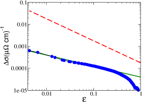
Figure 1: (Color online) Comparison between the experimental paraconductivity for a SmFeAsO_0.8F_0.2 sample studied in Ref. [gonnelli, ] (black circles) and the 2D (dashed line) and 3D (solid line) expressions of the AL paraconductivity [Eqs. (8,9)]. For the 3D paraconductivity a coherence length $\xi_{z}=19$ Å has been used, while for the 2D case the structural distance between layers $d=8.4$ Å has been inserted.

The fitting with Eq. (8) allows us to determine the precise value of $T_{c}$ and the coherence length $\xi_{z}$ of the SC fluctuations in the direction perpendicular to the FeAs layers. We find $T_{c}=51.4$ K and $\xi_{z}=19$ Å. One can also see that substantial SC fluctuations persist up to $\epsilon\approx(T-T_{c})/T_{c}\approx 0.4$, i.e., up to $20$ K above $T_{c}$. This fluctuating regime is therefore much larger than in conventional 3D superconductors and, despite the 3D behavior of the paraconductivity, calls for a relevant character of the layered structure and for a small planar coherence length. We point out that at even larger values of $\epsilon$ the paraconductivity drastically drops, in analogy with what found in cuprates (see, e.g., Ref. [caprara05, ], and references therein). The way paraconductivity deviates from the AL behavior in multiband systems also depends on the role of the other (non-critical) collective modes. In particular, it can be shown future that, when the intraband pairing is equally dominant in all bands, the paraconductivity mediated by the non critical modes may become sizable, and the experimental data should approach the pure AL contribution of the critical mode from above. This is not the case when the dominant pairing is interband and therefore it is not surprising that the data for the pnictide sample analyzed in this paper always lay below the AL straight line in Fig. 1.

In conclusion, we investigated the occurrence of SC fluctuations in a multiband system where interband pairing dominates, as appropriate for pnictides. In contrast to the case of dominant intraband mechanism (as, e.g., in MgB₂ varlamov ), in the present situation the HS decoupling must be accompanied with a proper rotation of the fermion fields which guarantees a Hermitian saddle-point action below $T_{c}$. The same rotation leads to a straightforward decoupling of the Gaussian fluctuations above $T_{c}$ in the hydrodynamic limit. Thus, despite the apparent complexity of the multiband structure in pnictides, we demonstrate that the AL expressions for paraconductivity stay valid not only as far as the functional temperature dependence is concerned, but also regarding the numerical prefactors. While in the BCS 2D case the prefactor stays universal, in the 3D case the only difference is that a suitable redefinition of the transverse coherence length has to be introduced. With this equipment, we considered the experimental resistivity data of the SmFeAsO_0.8F_0.2 sample studied in Ref. [gonnelli, ], finding that here fluctuations have a 3D character and extend far above $T_{c}$. Recently, an experimental workmarina on fluctuation conductivity in pnictides confirmed the wide fluctuating regime, even though fluctuations seem to have 2D character. Thus, further experiments are in order to confirm the nature of fluctuations in pnictides, and to assess the relevance of Cooper-pair fluctuations in these new superconductors.

Acknowledgments. We warmly thank D. Daghero and R. Gonnelli for providing us with the data of Ref. gonnelli . This work has been supported by PRIN 2007 (Project No. 2007FW3MJX003).

References

- (1) Y. Kamihara, T. Watanabe, M. Hirano, and H. Hosono, J. Am. Chem. Soc. 130, 3296 (2008).
- (2) See, e.g., T. Goko, et al. arXiv:0808.1425.
- (3) H. Ding, P. Richard, K. Nakayama, K. Sugawara, T. Arakane, Y. Sekiba, A. Takayama, S. Souma, T. Sato, T. Takahashi, Z. Wang, X. Dai, Z. Fang, G. F. Chen, J. L. Luo and N. L. Wang, Europhys. Lett. 83, 47001 (2008).
- (4) D. Daghero, M. Tortello, R. S. Gonnelli, V. A. Stepanov, N. D. Zhigadlo, J. Karpinski, arXiv:0812.1141.
- (5) L. Boeri, O. V. Dolgov, and A. A. Golubev, Phys. Rev. Lett. 101, 026403 (2008)
- (6) I. I. Mazin, D. J. Singh, M. D. Johannes, M. H. Du, Phys. Rev. Lett. 101, 057003 (2008);
- (7) V. Stanev, J. Kang and Z. Tesanovic, Phys. Rev. B78, 184509 (2008); R. Sknepnek, G. Samolyuk, Y. Lee, and J. Schmalian, Phys. Rev. B79, 054511 (2009).
- (8) A. V. Chubukov, D. Efremov, I. Eremin, Phys. Rev. B78, 134512 (2008); V. Cvetkovic and Z. Tesanovic, Europhys. Lett. 85, 37002 (2009).
- (9) A. Y. Liu, I. Mazin, and J. Kortus, Phys. Rev. Lett. 87, 087005 (2001).
- (10) A. Larkin and A. Varlamov, Theory of fluctuations in superconductors, (Clarendon Press, Oxford, 2005).
- (11) A. E. Koshelev, A. A. Varlamov and V. M. Vinokur, Phys. Rev. B72, 064523 (2005).
- (12) L. G. Aslamazov and A. I. Larkin, Phys. Lett. A 26, 238 (1968); Sov. Phys. Solid State 10, 875 (1968).
- (13) L. Benfatto, M. Capone, S. Caprara, C. Castellani, and C. Di Castro, Phys. Rev. B78, 140502(R) (2008).
- (14) For a list of references in the single-band case see, e.g., L. Benfatto, A. Toschi, and S. Caprara, Phys. Rev. B. 69, 184510 (2004).
- (15) S. Caprara, M. Grilli, B. Leridon, and J. Vanacken, Phys. Rev. B 79, 024506 (2009).
- (16) S. Caprara, M. Grilli, B. Leridon, and J. Lesueur, Phys. Rev. B 72, 107509 (2005).
- (17) L. Benfatto, S. Caprara, C. Castellani, L. Fanfarillo, and M. Grilli, unpublished.
- (18) I. Pallecchi, C. Fanciulli, M. Tropeano, A. Palenzona, M. Ferretti, A. Malagoli, A. Martinelli, I. Sheikin, M. Putti, and C. Ferdeghini, Phys. Rev. B79, 104515 (2009).