An Active Set Algorithm to Estimate Parameters in
Generalized Linear Models with Ordered Predictors
Abstract
In biomedical studies, researchers are often interested in assessing the association between one or more ordinal explanatory variables and an outcome variable, at the same time adjusting for covariates of any type. The outcome variable may be continuous, binary, or represent censored survival times. In the absence of precise knowledge of the response function, using monotonicity constraints on the ordinal variables improves efficiency in estimating parameters, especially when sample sizes are small. An active set algorithm that can efficiently compute such estimators is proposed, and a characterization of the solution is provided. Having an efficient algorithm at hand is especially relevant when applying likelihood ratio tests in restricted generalized linear models, where one needs the value of the likelihood at the restricted maximizer. The algorithm is illustrated on a real life data set from oncology.
Keywords: ordered explanatory variable, constrained estimation, least squares, logistic regression, Cox regression, active set algorithm, likelihood ratio test under linear constraints
1 Introduction
In many applied problems and especially in biomedical studies, researchers are interested in associating an outcome variable to several explanatory variables, typically via a generalized linear or proportional hazards regression model. Here, the explanatory variables or predictors may be continuous, nominal or ordered. Estimates of regression parameters can be obtained via maximizing a least-squares or (partial) likelihood function. Especially if the number of observations is small to moderate, researchers often encounter noisy estimates of the regression parameters, possibly leading to patterns in the regression estimates that violate the a-priori knowledge of a factor being ordered. In order to improve accuracy of estimates and efficiency of overall tests for associations, it is tempting to use the prior knowledge of orderings in some of the regression coefficients.
From a Bayesian perspective, receiving estimators in these type of problems is straightforward using Markov Chain Monte Carlo approaches. Pioneered in a linear model framework by Gelfand et al. (1992), Bayesian approaches have been proposed by Robert and Hwang (1996); Dunson and Neelon (2003); Dunson and Herring (2003). We also refer to the discussion in the latter two papers. To use Gibbs sampling to get the ordered predictor estimate in logistic regression, Holmes and Held (2006) combine the approach in Gelfand et al. (1992) with an auxiliary variable technique. Note that using e.g. flat priors on the regression coefficient vector it is straightforward to show that the maximum a posteriori estimator is equal to the constrained MLE introduced in Section 2.
Although conceptually straightforward, the implementation of these Bayesian approaches is not without fallacies. To not only get point estimates but also assess whether parameters are equal or strictly ordered across level of predictors, one needs to borrow from more frequentist approaches and “isotonize” unconstrained parameter estimates (Dunson and Neelon, 2003). Only then one can accommodate “flat regions”, i.e. successive estimates for ordered levels that are equal.
Although there exists vast literature on frequentist estimation subject to order restrictions (Robertson et al., 1988), estimation in the specific regression model discussed here has gained surprisingly little attention (Mukerjee and Tu, 1995). This may be due to the fact that setting up algorithms in these type of problems is generally difficult (Dunson and Neelon, 2003), and requires approaches that need to be adapted to specific problems, necessitating a vast literature for numerous cases of order restricted estimation. We mention Dykstra and Robertson (1982); Matthews and Crowther (1998); Jamshidian (2004); Tan et al. (2007); Taylor et al. (2007), or Balabdaoui et al. (2009) discussing computation of order restricted estimates in specific regression problems, and Terlaky and Vial (1998); Balabdaoui and Wellner (2004) or Rufibach (2007) for estimation of probability densities under order restrictions. Additionally, generalizations of the pool-adjacent-violaters algorithm (PAVA) to inclusion of continuous isotonic covariates are discussed in Bacchetti (1989); Morton-Jones et al. (2000); Ghosh (2007); Cheng (2009) in the context of “additive isotonic regression”. Estimation in this type of model is usually performed using the cyclical PAVA in connection with backfitting. However, note that we are not in this genuinely semiparametric setting, but rather the number of levels of an ordered factor is given a priori and remains fixed for any number of observations.
Recently, a type of algorithm, which has been around in optimization theory for some decades (Fletcher, 1987), has gained considerable attention in the statistical literature: active set algorithms. Dümbgen et al. (2007) use and generalize such an algorithm to compute a log-concave density not only from i.i.d. but even from censored data. An algorithm similar in spirit is the support reduction algorithm discussed in Groeneboom et al. (2008). The latter authors apply it to the estimation of a convex density and to Gaussian deconvolution. A slight generalization of the support reduction algorithm is used to estimate a convex-shaped hazard function in Jankowski and Wellner (2009). Beran and Dümbgen (2009) extend active set algorithms to the estimation of smooth bimonotone functions. They illustrate their algorithm on regression with two ordered covariates, so also treating the example dealt with in this paper. However, Beran and Dümbgen (2009) only consider least squares or least absolute deviation estimation, and at most two ordered factors. In this paper, we propose an algorithm for an arbitrary number of ordered factors, and we also provide a characterization of the solution.
A key feature of an active set algorithm is, that although iterative, it terminates after finitely many steps, and that the solution is finally found via an unconstrained optimization. This implicitly implies that, as opposed to some Bayesian approaches (Dunson and Neelon, 2003), the active set algorithm is not hurt if estimates of subsequent levels turn out to be equal. In Section 2 we show that the estimation of a regression function in generalized linear models (GLM) under the above ordered factor restriction can be easily performed using such an active set algorithm.
Optimal scaling
A reviewer drew our attention to optimal scaling, where one seeks to assign numeric values to categorical variables in some optimal way, see e.g. Breiman and Friedman (1985); Gifi (1990); Hastie and Tibshirani (1990), or applied to modeling interactions in Van Rosmalen et al. (2009). In Gifi (1990, Section 2) categories of the original categorical variables are replaced by “category quantifications”, and from then on the variables are considered to be quantitative. Note that in the approach discussed in this paper, one does not necessarily look for an optimal transformation, but rather imposes a priori knowledge on a given ordered predictor. In the example analyzed in Section 9 it seems plausible that a higher tumor or nodal stage is associated with a higher risk of experiencing a second primary tumor.
Ordered predictors
While the treatment of quantitative and grouped predictors in regression models is straightforward, we briefly review alternative approaches that can be applied to deal with an ordered explanatory variable . Let us assume the levels of are coded as where and the levels are increasingly ordered, i.e. .
The most straightforward way to incorporate as a predictor is simply to ignore the information about the groups and consider it a quantitative variable. This approach implicitly assumes that the group levels represent a true dimension, with intervals measured between adjacent categories that correspond to the chosen coding. If the ordinal values are arbitrarily assigned rather than actually measured, the regression coefficient is then difficult or impossible to interpret.
Supposedly the most prevalent approach to incorporate an ordered predictor in a regression model is to introduce dummy variables where . This approach ignores the additional knowledge of having ordered levels, entailing that the estimated parameters corresponding to the above dummy variables may not be increasingly ordered. This is especially relevant in small sample studies, where noisy estimates may confuse the proper order of dummy variable coefficients.
To simplify interpretation of models, especially when interactions are to be incorporated, researchers sometimes resort to dichotomizing a grouped factor, i.e. introducing only one dummy variable , for some . Here, the additional knowledge about the ordered levels is not used and may cause a substantial loss of predictive information (Steyerberg, 2009, Section 9.1).
Another choice may be polynomial contrasts. One then introduces new variables . To avoid correlated estimators and therefore mutually dependent tests when doing variable selection, researchers generally prefer to modify the design matrix in order to get orthogonal polynomial contrasts. The function as.ordered() in R (R Development Core Team, 2009) does this by default.
Gertheiss and Tutz (2008) proposed a ridge-regression related approach to perform regression with ordered factors. Consider the predictor with ordered categories and the linear regression model
| (1) | |||||
For simplicity, we do not consider an intercept and only one ordered factor. The vectors are vectors of dummy variables corresponding to the levels of , is the design matrix with the ’s as columns, is the response and an i.i.d. noise vector where . Note that for reasons of identifiability, Gertheiss and Tutz (2008) assume and therefore omit in (1).
Instead of maximizing the original likelihood over , Gertheiss and Tutz (2008) instead propose to maximize a penalized version of :
| (2) |
Here, is a tuning parameter. The solution to (2) can be explicitly computed as
| (3) |
for a fixed and specified matrix . The idea is that is assumed to change slowly for adjacent categories, a property of that is “encouraged” by the shrinkage estimator (3). However, note that may still contain two adjacent estimates such that , a somewhat undesired feature in this setting. Furthermore, if we choose as our reference level (and therefore implicitly assume that ), it seems reasonable to demand for the estimated coefficients that they are all positive, what is not ensured by using (3). Finally, further considerations are necessary to determine the tuning parameter .
Consider Setting (1) as before. In this paper, we introduce an algorithm to solve the following problem: Maximize assuming that and under the constraint that
| (4) |
so that we receive non-negative and adequately ordered estimated parameters for the factor levels. This approach is appealing since the available knowledge (or our “prior belief”) is precisely exploited. Furthermore, constraining the space of allowed parameters can be interpreted as regularizing the estimator, implying higher accuracy of the constrained estimate (Dunson and Neelon, 2003). This is especially relevant in small samples. As can be seen from (4), we can estimate parameters for an ordered factor such that the constraints are enforced, unlike in Gertheiss and Tutz (2008) where the violation of these inequalities is only penalized. In the latter approach the violation of the first of the above inequalities, the non-negativity constraint, is not even penalized. In addition, our estimator is fully automatic, i.e. no arbitrary choices such as the coding of levels, the determination of a cutoff to pool levels, or the selection of a tuning parameter (such as above) or bandwidth are necessary.
Testing in order restricted models
There is a vast literature on likelihood ratio testing in models under linear equality and inequality constraints. For a discussion and further references on (exact) testing under restrictions in the ordinary linear regression model see Perlman (1969), Wolak (1987) and Shapiro (1988). Silvapulle (1994) and Fahrmeir and Klinger (1994) generalize these results to generalized linear models, especially logistic and Cox regression. As can be seen from (14) below, any likelihood ratio test (LRT) is constructed as the difference of the likelihoods at the unrestricted and the restricted maximizer of the (partial) log-likelihood function, which entails that one needs an algorithm to compute the restricted maximizer. Silvapulle (1994, Section 4) describes an ad-hoc approach to find the constrained estimators. However, his algorithm is non-standard and tedious to apply (Silvapulle, 1994, p. 856). The active set algorithm described here is a general framework able to tackle general optimization problems under constraints and therefore able to compute the restricted estimators in the above mentioned tests very efficiently. This facilitates the application of LRTs in this type of problem.
Statistical inference and asymptotics
Typically, deriving asymptotic properties of shape-constrained estimators is hard, but the starting point in all these problems (Groeneboom et al., 2001; Balabdaoui and Wellner, 2004; Dümbgen and Rufibach, 2009) is a characterization of the estimator, since all the estimators are defined as maximizer of some rather involved function. The most prominent example of a theoretical treatment of a shape constrained estimator via its characterization is the greatest convex minorant that characterizes the estimator of a monotone density (Grenander, 1956). In Section 6 we characterize the solution in our problem. Besides being the starting point for a more thorough analysis, a characterization also allows to check whether an algorithm actually delivers the correct solution.
Our contribution
We propose an active set algorithm to find estimators in GLMs with ordered predictors. The estimators strictly comply with the constraints and are found very efficiently, and in a finite number of steps. For identifiability reasons, most regression approaches assume that the coefficient corresponding to the lowest level of an ordered factor is equal to 0. Our approach ensures that all coefficients corresponding to higher levels are in fact non-negative as well. In addition, neither the estimator nor the proposed algorithm needs a tuning parameter. Having an efficient algorithm at hand that provides restricted estimates facilitates the application of LRTs to check whether ordered predictors should be included in the model. In addition, we provide a characterization of the estimator. This serves (i) as a benchmark to verify that the algorithm indeed delivers the maximizer, (ii) gives some insight in the structure of the estimator and (iii) marks the starting point for a more thorough (asymptotic) analysis.
Organization of the paper
A general formulation of the problem is given in Section 2. Some examples of GLMs that illustrate our new approach are discussed in Section 3. A description of the active set algorithm adapted to our problem is given in Section 4. There exist special cases of the problem that allow one to find the linear regression estimator more easily than using the active set algorithm, discussed in Section 5. A characterization of the solutions is given in Section 6. Some indications on statistical inference are provided in Section 7. Literature on likelihood-ratio testing to check whether an ordered factor should be included in the model is briefly discussed in Section 8. A real data example from oncology is analyzed in Section 9. Finally, a more technical description of the algorithm and proofs are postponed to the Appendix.
2 Setup
We consider the general regression problem of modeling an outcome based on some feature vector . Therefore, we are given a set of observations, for . Write
| and |
where , . The predictors are denoted by for . Throughout the exposition, and are considered to be fixed.
In general, for given and , we seek to maximize a real–valued concave criterion function
over , yielding an estimated parameter vector . Note that to define our estimator and to derive the characterization in Section 6, a model needs no further specification that goes beyond the function . Ordinary, i.e. unordered, factors are assumed to be already coded as dummy variables, so they are considered quantitative. If an intercept is to be taken into the model, we simply assume it to be a quantitative variable of all ’s. Let denote the number of quantitative predictors and suppose that the last predictors , are ordered factors, each with levels (so ). Furthermore, the coding is assumed such that , where a higher number corresponds to a “higher” level of the ordered factor . Introduce the sets of indices and for . Clearly, the case (no quantitative variables in the model) is not excluded. However, we assume to have at least one ordered factor, i.e. which immediately implies . In order to respect the ordinal character of each of the factors we estimate based on a new data matrix . This latter matrix is obtained via modifying the original data matrix by adding
dummy variables for the levels of the ordered factors. We then constrain optimization of the updated functional to the constrained space of parameters
| (5) |
Here, is the coefficient of the dummy variable corresponding to the level of the -th ordered factor, and . For ease of notation, we define . Constraining estimation to ensures that the estimated parameter corresponding to a “higher” level of an ordered factor is at least as large as those of “lower” levels and all estimated parameters are non-negative. Note that our approach also adds something new if we have an ordered factor with only two levels (note that we always lose the level attributed to the baseline), namely that for this ordered factor.
3 Examples
We briefly specify the GLMs we provide algorithms for. Extensions to other criterion functions are straightforward.
Linear regression
Here, and we estimate via maximizing the criterion function over all . This latter function is defined as
Here, denotes the -th row vector of . We emphasize that given there is no need to further specify a model for the data.
Logistic regression
In this case, . Using maximum likelihood estimation (MLE) we obtain the log–likelihood function
Cox regression
Here, we have observations for . Clearly, are the failure times (possibly unobserved), the censoring times, event has happened and is the feature vector as before. If we introduce the observed time for each unit, let
denote the number of individuals at risk after time , . The partial likelihood according to Cox (1972) is then
Introducing for and letting be the observed (assumed to be distinct, for simplicity) event times, we then easily deduce the log-likelihood function:
where is the above expression belonging to the -th failure time, .
Properties of the maximization problems
Let us introduce the constrained
| (6) |
and the unconstrained
maximizers. The conditions on fixed response and design matrix under which exist and are unique in logistic regression are well studied (Albert and Anderson, 1984; Santner and Duffy, 1986). Silvapulle and Burridge (1986) specify necessary and sufficient conditions for the MLE to exist in logistic and Cox regression. Since the set is a closed convex cone, the estimators exist and are unique for at least under the same conditions as those for . Conditions for consistency and asymptotic normality of MLEs in GLMs are provided in Fahrmeir and Kaufmann (1985). In this paper we assume that our design matrix is such that is concave and coercive for .
4 Active set algorithm to compute
In Fletcher (1987) an active set algorithm is described, a useful tool for constrained optimization problems. In connection with likelihood ratio tests (see Section 8) we came across Silvapulle (1994). In Section 4 of this latter paper, it seems as if a version of the active set algorithm is described. However, instead of directly computing the “active set” in each iteration (see below), a crude and computationally expensive “all-subset search” is proposed. In the context of mixture models, the algorithm discussed by Groeneboom et al. (2008) can also be interpreted as a variant of an active set algorithm.
In Section 3 of Dümbgen et al. (2007) the general principle of active set algorithms is described in detail, complemented by a discussion of its validity. Here, we therefore limit ourselves to the discussion of the main features and points relevant for the application of the active set algorithm to find the ’s. We briefly sketch the idea of an active set algorithm, and refer to A for a detailed technical exposition of the algorithm for the problem treated here.
Let denote the number of constraints that compose , the function to be maximized and its maximizer, see Section 3. Define for any index set the linear subspace
The function maps the indices and of the dummy variables forming the ordered factors to the number of constraining inequalities, see (16) in A. The crucial assumption for an active set algorithm is that we have another algorithm available that for any (efficiently) computes
provided that . Subspaces of the parameter space are considered when violations of the initial constraints appear in the algorithm. In this case, the active set algorithm varies in a deterministic way, until finally . In order to tailor an active set algorithm to a specific problem, the above maximization on a subspace is crucial. In our regression with ordered covariates setting, we show in A (see Table 4) that three types of subspaces have to be dealt with, depending on the specific violation that occurs.
It is important to realize that by design, the main routine of an active-set algorithm does not need a stopping criterion as e.g. Newton-type algorithms. Once the algorithm has identified the set that corresponds to the solution , it performs an unrestricted maximization (here, a stopping criterion may be necessary), which at least in the linear, logistic and Cox regression examples is unproblematic. Verification that a given is the maximizer can be done by means of Theorem 3.1 in Dümbgen et al. (2007). Additionally, since there are only finitely many subsets of , the algorithm terminates after finitely many steps.
5 Special case: An almost explicit solution
To be able to state the following results concisely, let us introduce for every ordered factor the set of indices where the equality constraint is active:
for all .
In this section, we restrict our attention to the case of linear regression with only one ordinal predictor. If in addition , that means the constrained estimator has only strictly positive entries anyway, then simplifies such that can be found via solving (7).
Lemma 5.1.
If , and , the estimator is
| (7) | |||||
where for
| and |
The proof of this lemma is postponed to B.
The solution to (7) can easily be computed using the PAVA (Barlow et al., 1972; Robertson et al., 1988). This latter algorithm performs at most iterations until the vector is found.
One of the initial motivations to analyze regression with ordered predictors, and the reason why we included this very specific example, was to see whether this simple and appealing structure can be carried forward to the more general problem of more ordered factors and additional quantitative variables. However, since (i) we were not able to construct a generalized PAVA algorithm that solves our problem and (ii) we are not only interested in the least-squares problem but also treat GLMs, we switched to an active set algorithm.
6 Characterization of the solution
There are two main purposes of providing a characterization of the estimator : (i) knowing the structure of the maximizer of allows one to cross-check the validity of the proposed active-set algorithm and to check whether it has found the correct maximizer of . (ii) It is well-known that in such constrained estimation problems, the key to deriving asymptotic properties of the estimator such as consistency or rate of convergence is a characterization in terms of directional derivatives, see the discussion in Section 1.
To be able to state the following theorem properly, we introduce the function that maps the original indices to the column number of the respective dummy variable in , or equivalently, to the index that corresponds to the entry of the vector that corresponds to . Specifically, this function is for any and ,
| (8) | |||||
By we denote the inverse of this function, i.e. the function that maps the position of the entry of to the indices and . Now, for each let be the vector of distinctive strictly positive values of for every and any . Using these definitions we split any vector into the following blocks:
| = | (coefficients of quantitative variables), | ||
| = | , | ||
| = | {all indices s.t. for }, | ||
where for each . Here, denotes the dimension of a vector or the number of elements in a set. Note that . Using these blocks, we are now able to formulate the characterization of the solution.
Theorem 6.1.
An arbitrary vector maximizes the concave function if and only if it fulfills the following conditions:
| (9) | |||||
| (10) | |||||
| (11) |
Note that the entries of the gradient at the active constraints , , are not needed to characterize the solution since always equals 0 at these positions. Furthermore, the theorem immediately implies
| (12) |
for and .
To illustrate Theorem 6.1, consider the following example: For observations we generated a dataset with standard normally distributed errors, three quantitative variables, one (unordered) factor (with three levels) and one ordered factor (with eight levels). The model we stipulated to generate the response was
where for and , each level of any factor (whether ordered or unordered) has the same number of observations and these are randomly allocated to the observations. Finally, for . The resulting (constrained) linear regression estimates are given in Table 1. Note that for comparison we also added columns for the estimator which is computed similarly to , but without the positivity restriction . For this estimator, a characterization similar to that in Theorem 6.1 can be given using exactly the same approach.
| Var | Level | |||||||||
| quant | 2 | 2.13 | 0 | 2.12 | 0 | 0 | 2.08 | 0 | 0 | |
| quant | -3 | -2.95 | 0 | -2.94 | 0 | 0 | -2.96 | 0 | 0 | |
| quant | 0 | 0.19 | 0 | 0.18 | 0 | 0 | 0.17 | 0 | 0 | |
| fact1 | 2 | 1 | 1.06 | 0 | 1.08 | 0 | 0 | 0.88 | 0 | 0 |
| fact1 | 3 | 1 | 1.53 | 0 | 1.41 | 0 | 0 | 1.23 | 0 | 0 |
| ord1 | 2 | 0 | -0.85 | 0 | -0.78 | 0 | 0 | 0 | -26.86 | -26.86 |
| ord1 | 3 | 2 | 3.55 | 0 | 1.99 | 79.8 | 79.8 | 2.19 | 79.23 | 52.38 |
| ord1 | 4 | 2 | 1.67 | 0 | 1.99 | -13.57 | 66.23 | 2.19 | -12.66 | 39.71 |
| ord1 | 5 | 2 | 0.60 | 0 | 1.99 | -65.85 | 0.39 | 2.19 | -65.3 | -25.59 |
| ord1 | 6 | 2 | 1.94 | 0 | 1.99 | -0.39 | 0 | 2.19 | -1.27 | -26.86 |
| ord1 | 7 | 5 | 4.41 | 0 | 4.47 | 0 | 0 | 4.65 | 0 | -26.86 |
| ord1 | 8 | 5 | 4.55 | 0 | 4.60 | 0 | 0 | 4.79 | 0 | -26.86 |
In this example, we get the following quantities: , , , , , , , and finally
The notation in Table 1 is shorthand for the cumulative sum of any vector :
The values of the least-squares criterion function for the three estimates are
and .
Let us now illustrate Theorem 6.1. For either quantitative variables or dummy variables corresponding to unordered factors (which in our context are conceptually equivalent), the respective entry of the gradient is always 0. As for the ordered factor, for the entries where the positivity constraint is active (i.e. the elements in ), the gradient has a value which is not used (and not necessary) for a characterization of . The sets defined above are for the simulated example:
| = | = | = | ||||||
| = | = | = |
7 Statistical inference
Having shown how to compute estimators for , the question arises how to perform (frequentist) statistical inference in these models. Deriving consistency, rate of convergence and limiting distributions for estimators similar to under standard assumptions is known to be non-trivial. It is therefore not clear how to construct e.g. confidence intervals for our estimated parameters of the ordered factor. By using the characterization given in Section 6, one should be able to derive rates of convergence and even the limiting distribution of as in a suitably specified model, thereby generalizing the results of Brunk (1970) and Wright (1981) for isotonic regression to our more general setting. This, together with a generalization of the likelihood ratio tests introduced in Section 8 to an arbitrary number of ordered factors, is subject to ongoing research.
8 Testing for the presence of constraints
There is a vast literature on likelihood ratio testing in models under linear equality and inequality constraints. For a discussion and further references on (exact) testing under restrictions in the ordinary linear regression model see Perlman (1969), Wolak (1987) and Shapiro (1988). Silvapulle (1994) and Fahrmeir and Klinger (1994) generalize these results to generalized linear models, especially logistic and Cox regression. Suppose a researcher wants to test the following hypotheses:
| (13) |
Note that the estimator under can be computed via an unrestricted maximization. It corresponds to a maximization using a modified design matrix with the columns omitted. Since under we need to consider an unrestricted estimator, we have to constrain attention either to (i) only one ordered factor or (ii) a test of inclusion of all ordered factors against their entire exclusion from the model. The potential influence of the additional ordered factor(s) on the response is assessed with . In notation similar to Silvapulle (1994), the above hypotheses translate to
where here is the matrix chosen such that
Following the development in Silvapulle (1994), the likelihood ratio test statistic to test the Hypotheses (13) is defined as
| (14) |
The distribution of is a mixture of distributions. The weights are in principle fully specified, however, in general hard to compute (Wolak, 1987). As a remedy, one can either use exact Monte Carlo weights (Wolak, 1987) or bounds on the -value for the above test (Silvapulle, 1994, Proposition 1).
As can be seen from (14) any LRT is constructed as the difference of the likelihoods at the unrestricted and the restricted maximizer of the (partial) log-likelihood function, which entails that one needs an algorithm to compute the restricted maximizer. Silvapulle (1994, Section 4) describes an ad-hoc approach to find constrained estimators. However, his algorithm is non-standard and tedious to apply (Silvapulle, 1994, p. 856). The active set algorithm described here is a general framework able to tackle general optimization problems under constraints and able to compute the restricted estimators in the above mentioned tests very efficiently.
9 A real data example
We illustrate our new algorithm using a data set from oncology, initially analyzed in Taussky et al. (2005). The goal of the study was to assess the impact of treatment- and patient-related factors on the risk of developing a second primary tumor (SPT) of the upper aerodigestive tract within three years after initial therapy, in head-and-neck cancer patients. For a subset of 231 patients that had either been observed at least three years without SPT or experienced an SPT before three years, the endpoint
was defined and modeled using multiple logistic regression. The explanatory variables are described in Table 2.
| Variable | Type | Levels (first mentioned = baseline) |
|---|---|---|
| Intercept (inter) | constant | |
| Age (age) | continuous (standardized) | |
| Treatment (tmt) | factor | Chemotherapy (CT) yes, CT no |
| Radiotherapy (rt) | factor | concomitant boost (CB), hyperfractionation (HF) |
| Sex (sex) | factor | female, male |
| Tumor stage (t) | ordered factor | |
| Nodal stage (n) | ordered factor | |
| Performance status (ps) | ordered factor | “stage greater than 2” |
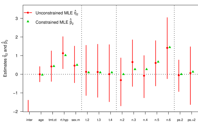
Researchers assume in general that higher tumor stage, nodal stage, and performance status correspond to a higher risk of experiencing a SPT. It seems therefore appropriate to use our constrained estimator in this setting. In Figure 1, the unconstrained and constrained estimators and are displayed (dot and triangle, respectively) as well as profile likelihood confidence intervals for (). Values of the likelihoods were and .
Estimates for quantitative predictors, i.e. those for age, treatment, radiotherapy and sex turned out to be very similar for and . On the other hand, the “prior belief” or assumption of non-negative and increasing estimates for the levels of the ordered factors tumor and nodal stage and performance status was violated by the unconstrained estimator and “corrected” by .
The original analysis in Taussky et al. (2005) focused on identifying factors that influence the occurrence of SPT. Variables were not taken into account as ordered factors, but were dichotomized. For comparison, we also computed the restricted and unrestricted estimates in this setting, see Table 3. It turns out that parameter estimates and corresponding odds ratios (OR) for the two approaches were similar, except for the nodal status. Note that the effect of tumor stage is reversed, compared to the case where we consider all factor levels (and do not only dichotomize), compare Figure 1.
| Variable | Type | Levels | OR | OR | ||
|---|---|---|---|---|---|---|
| Intercept | constant | -2.56 | -2.72 | |||
| Age | factor | , | -0.19 | 0.83 | -0.20 | 0.82 |
| Treatment | factor | CT yes, CT no | 0.41 | 1.51 | 0.42 | 1.53 |
| Radiotherapy | factor | CB, HF | 1.03 | 2.81 | 0.99 | 2.70 |
| Sex | factor | female, male | 0.51 | 1.67 | 0.49 | 1.63 |
| Tumor stage | ordered factor | , | -0.21 | 0.81 | 0.00 | 1.00 |
| Nodal stage | ordered factor | , | 0.26 | 1.29 | 0.27 | 1.31 |
| Performance status | ordered factor | , | 0.37 | 1.44 | 0.40 | 1.49 |
10 Extensions
It is straightforward to generalize the set to
for arbitrary real numbers . Using such a more general parameter space could be beneficial in connection with finding the minimum effective dose in dose-response models. The dose levels would then take the role of an ordered factor (Wang and Peng, 2007). Our new approach easily allows us to incorporate further predictors of any of the three types described in the introduction to model the response.
Modeling a factor with decreasing levels can be achieved by reversing the coding of the corresponding ordered factor, using the algorithm under the constraint of increasing levels and finally re-reversing the order of the estimates in the vector . Using this approach, it is straightforward to find the solutions for all combinations of possible orderings of, say, three ordered factors. By computing the value of the criterion function for all these resulting coefficient vectors, one can find the one with the lowest criterion value, an approach related to finding a global maximum in the criterion function described in van der Kooij et al. (2006).
Generalizations to further criterion functions, such as other GLMs or least absolute deviation regression with ordered covariates, are straightforward. As for the latter problem, we suggest smoothly approximating the not everywhere differentiable criterion function, as previously discussed in Beran and Dümbgen (2009).
11 Acknowledgments
The initial motivation for this research grew out of discussion with Lutz Dümbgen while preparing exercises for his lecture “Optimization” during summer semester 2006 at the University of Bern. I thank Leonhard Held for discussions about the Bayesian perspective of the problem, Sarah Haile for proofreading the final version, and my former employer, the Swiss Group for Clinical Cancer Research (SAKK), for the permission to use the data of Taussky et al. (2005).
Appendix A Details of the active set algorithm
In this section, we complement the description of the algorithm indicated in Section 2. Recall the sets of indices and for .
In order to respect the ordinal character of each of the factors we introduced in Section 2 the new data matrix by adding dummy variables for the ordered factors, such that
for dummy variables
The function is given in (8). With the above version of coding, is considered the reference level for every ordered factor and the resulting design matrix is now an element of where
Again, we denote by the -th row of , i.e. the values of the “dummyfied” predictors for the -th observation. In order to respect the ordinal character of each of the factors we then constrain optimization of the updated functional to the space of parameters given in (5).
We write as placeholder for any of the functions or (for ease of notation we omit the dependence on ) and the aim is to find for given response vector and matrix of predictors the vector
To fit the constrained maximization problem (6) into the framework of Dümbgen et al. (2007), we write the set given in (5) as
for vectors . For ease of notation, we have enumerated the constraining inequalities
from , where
The function that maps the original indices to the “inequality index” is given by
| (16) | |||||
so that the inequalities can be written as
for and . The vectors for any are received via
Note that all these vectors are linearly independent. Define for any index set the linear subspace
and for the set of “active constraints”:
Maximization on subspace
The crucial assumption for an active set algorithm is that we have an algorithm available that for any (efficiently) computes
provided that , see Section 4. For simplicity and without loss of generality, fix . Then, for a given the following situations can cause a non-empty set :
Case Violation(s) Corresponding set 1 2 3
Note that the situation for any can be treated analogously to Case 2 in Table 4.
To compute the unrestricted maximizer in the three cases given in Table 4, the strategy is to suitably modify the design matrix . Precisely, we show how to construct new data matrices and a new corresponding function (here, stands for the corresponding case in Table 4) for a given in the three cases of Table 4 such that can be immediately derived from
| (17) |
It is crucial to realize that the maximization in (17) is unconstrained and the following arguments show that in all considered cases. In what follows, we explicitly state the unconstrained maximization problem, assuming that only the case under consideration is present. Apparent combinations of these basic strategies are necessary in case more than one of the three cases described in Table 4 are present.
Case 1
Writing down the maximization problem (17) explicitly, we get
with
where in general is the matrix with the -th column omitted and is the criterion function corresponding to , but based on the design matrix .
Case 2
Roughly, the strategy here is to add up the dummy variables corresponding to the violating constraints, compute the unconstrained maximizer and then “blow up” the resulting estimator again. To see this, consider
with
Case 3
Repeating the above computations, we derive
where
Appendix B Proofs
Proof of Lemma 5.1
First, observe that for ,
The function can then be written as
The minimum of the latter expression under the constraint can easily be found using PAVA.
Proof of Theorem 6.1
Before coming to the actual proof, we state a necessary lemma.
Lemma B.1.
Let be two vectors having the following properties:
| (18) | |||||
| (19) | |||||
| (20) |
Then
First, we prove that if maximizes over , then (9)-(10) are fulfilled. To this end, let be small enough and let be a vector such that . Since maximizes the concave function we have
which entails
| (21) |
We then get (9)-(11) using the following perturbation functions:
for all and where we defined and . Now suppose we are given a vector that fulfills (9)-(11). We then have to show that
From convex analysis, it is well known that this is equivalent to show
| (22) | |||||
| (23) |
for arbitrary vectors such that . Now compute
| (24) | |||||
The second term disappears due to (12). As for the first term, we invoke Lemma B.1 where takes the role of and that of to finally deduce that (24) is at most 0.
Proof of Lemma B.1
References
- Albert and Anderson (1984) Albert, A. and Anderson, J. A. (1984). On the existence of maximum likelihood estimates in logistic regression models. Biometrika 71 1–10.
- Bacchetti (1989) Bacchetti, P. (1989). Additive isotonic models. J. Amer. Statist. Assoc. 84 289–294.
- Balabdaoui et al. (2009) Balabdaoui, F., Rufibach, K. and Santambrogio, F. (2009). Least squares estimation of two ordered monotone regression curves. J. Nonparametr. Stat., to appear .
- Balabdaoui and Wellner (2004) Balabdaoui, F. and Wellner, J. (2004). Estimation of a -monotone density, part 2: algorithms for computation and numerical results. Tech. rep., Technical report 460, Department of Statistics, University of Washington. Available at http://www.stat.washington.edu/www/research/reports/2004/tr460.pdf.
- Barlow et al. (1972) Barlow, R. E., Bartholomew, D. J., Bremner, J. M. and Brunk, H. D. (1972). Statistical inference under order restrictions. The theory and application of isotonic regression. John Wiley & Sons, London-New York-Sydney. Wiley Series in Probability and Mathematical Statistics.
- Beran and Dümbgen (2009) Beran, R. and Dümbgen, L. (2009). Least squares and shrinkage estimation under bimonotonicity constraints. Statistics and Computing to appear.
- Breiman and Friedman (1985) Breiman, L. and Friedman, J. H. (1985). Estimating optimal transformations for multiple regression and correlation. J. Amer. Statist. Assoc. 80 580–619. With discussion and with a reply by the authors.
- Brunk (1970) Brunk, H. D. (1970). Estimation of isotonic regression. In Nonparametric Techniques in Statistical Inference (Proc. Sympos., Indiana Univ., Bloomington, Ind., 1969). Cambridge Univ. Press, London, 177–197.
- Cheng (2009) Cheng, G. (2009). Semiparametric additive isotonic regression. J. Statist. Plann. Inference 139 1980–1991.
- Cox (1972) Cox, D. R. (1972). Regression models and life-tables. J. Roy. Statist. Soc. Ser. B 34 187–220. With discussion by F. Downton, Richard Peto, D. J. Bartholomew, D. V. Lindley, P. W. Glassborow, D. E. Barton, Susannah Howard, B. Benjamin, John J. Gart, L. D. Meshalkin, A. R. Kagan, M. Zelen, R. E. Barlow, Jack Kalbfleisch, R. L. Prentice and Norman Breslow, and a reply by D. R. Cox.
- Dümbgen et al. (2007) Dümbgen, L., Hüsler, A. and Rufibach, K. (2007). Active set and EM algorithms for log-concave densities based on complete and censored data. Tech. rep., University of Bern. Available at arXiv:0707.4643.
- Dümbgen and Rufibach (2009) Dümbgen, L. and Rufibach, K. (2009). Maximum likelihood estimation of a log-concave density and its distribution function. Bernoulli 15 40–68.
- Dunson and Herring (2003) Dunson, D. B. and Herring, A. H. (2003). Bayesian inferences in the Cox model for order-restricted hypotheses. Biometrics 59 916–923.
- Dunson and Neelon (2003) Dunson, D. B. and Neelon, B. (2003). Bayesian inference on order-constrained parameters in generalized linear models. Biometrics 59 286–295.
- Dykstra and Robertson (1982) Dykstra, R. L. and Robertson, T. (1982). An algorithm for isotonic regression for two or more independent variables. Ann. Statist. 10 708–716.
- Fahrmeir and Kaufmann (1985) Fahrmeir, L. and Kaufmann, H. (1985). Consistency and asymptotic normality of the maximum likelihood estimator in generalized linear models. Ann. Statist. 13 342–368.
- Fahrmeir and Klinger (1994) Fahrmeir, L. and Klinger, J. (1994). Estimating and testing generalized linear models under inequality restrictions. Statist. Papers 35 211–229.
- Fletcher (1987) Fletcher, R. (1987). Practical methods of optimization. 2nd ed. A Wiley-Interscience Publication, John Wiley & Sons Ltd., Chichester.
- Gelfand et al. (1992) Gelfand, A. E., Smith, A. F. M. and Lee, T.-M. (1992). Bayesian analysis of constrained parameter and truncated data problems using Gibbs sampling. J. Amer. Statist. Assoc. 87 523–532.
- Gertheiss and Tutz (2008) Gertheiss, J. and Tutz, G. (2008). Penalized regression with ordinal predictors. Tech. Rep. 15, Ludwig-Maximilians-University, Munich.
- Ghosh (2007) Ghosh, D. (2007). Incorporating monotonicity into the evaluation of a biomarker. Biostatistics 8 402–413.
- Gifi (1990) Gifi, A. (1990). Nonlinear multivariate analysis. Wiley Series in Probability and Mathematical Statistics: Probability and Mathematical Statistics, John Wiley & Sons Ltd., Chichester. With a foreword by Jan de Leeuw, Edited and with a preface by Willem Heiser, Jacqueline Meulman and Gerda van den Berg.
- Grenander (1956) Grenander, U. (1956). On the theory of mortality measurement. II. Skand. Aktuarietidskr. 39 125–153 (1957).
- Groeneboom et al. (2001) Groeneboom, P., Jongbloed, G. and Wellner, J. A. (2001). Estimation of a convex function: characterizations and asymptotic theory. Ann. Statist. 29 1653–1698.
- Groeneboom et al. (2008) Groeneboom, P., Jongbloed, G. and Wellner, J. A. (2008). The support reduction algorithm for computing non-parametric function estimates in mixture models. Scand. J. Statist. 35 385–399.
- Hastie and Tibshirani (1990) Hastie, T. J. and Tibshirani, R. J. (1990). Generalized additive models, vol. 43 of Monographs on Statistics and Applied Probability. Chapman and Hall Ltd., London.
- Holmes and Held (2006) Holmes, C. C. and Held, L. (2006). Bayesian auxiliary variable models for binary and multinomial regression. Bayesian Anal. 1 145–168 (electronic).
- Jamshidian (2004) Jamshidian, M. (2004). On algorithms for restricted maximum likelihood estimation. Comput. Statist. Data Anal. 45 137–157.
- Jankowski and Wellner (2009) Jankowski, H. K. and Wellner, J. A. (2009). Computation of nonparametric convex hazard estimators via profile methods. J. Nonparametr. Stat., to appear 21 505–518.
- Kosorok (2008) Kosorok, M. R. (2008). Bootstrapping in Grenander estimator. In Beyond parametrics in interdisciplinary research: Festschrift in honor of Professor Pranab K. Sen, vol. 1 of Inst. Math. Stat. Collect. Inst. Math. Statist., Beachwood, OH, 282–292.
- Matthews and Crowther (1998) Matthews, G. and Crowther, N. (1998). Theory and methods a maximum likelihood estimation procedure for the generalized linear model with restrictions. South African Statist. J. 32 119–144.
- Morton-Jones et al. (2000) Morton-Jones, T., Diggle, P., Parker, L., Dickinson, H. O. and Binks, K. (2000). Additive isotonic regression models in epidemiology. Stat. Med. 19 849–859.
- Mukerjee and Tu (1995) Mukerjee, H. and Tu, R. (1995). Order-restricted inferences in linear regression. J. Amer. Statist. Assoc. 90 717–728.
- Perlman (1969) Perlman, M. D. (1969). One-sided testing problems in multivariate analysis. Ann. Math. Statist. 40 549–567.
-
R Development Core Team (2009)
R Development Core Team (2009).
R: A Language and Environment for Statistical Computing.
R Foundation for Statistical Computing, Vienna, Austria.
ISBN 3-900051-07-0.
URL http://www.R-project.org - Robert and Hwang (1996) Robert, C. P. and Hwang, J. T. G. (1996). Maximum likelihood estimation under order restrictions by the prior feedback method. J. Amer. Statist. Assoc. 91 167–172.
- Robertson et al. (1988) Robertson, T., Wright, F. T. and Dykstra, R. L. (1988). Order restricted statistical inference. Wiley Series in Probability and Mathematical Statistics: Probability and Mathematical Statistics, John Wiley & Sons Ltd., Chichester.
- Rufibach (2007) Rufibach, K. (2007). Computing maximum likelihood estimators of a log-concave density function. J. Statist. Comp. Sim. 77 561–574.
-
Rufibach (2009)
Rufibach, K. (2009).
OrdFacReg: Least squares, logistic, and Cox-regression with
ordered predictors.
R package version 1.0.1.
URL http://www.biostat.uzh.ch/aboutus/people/rufibach.html - Santner and Duffy (1986) Santner, T. J. and Duffy, D. E. (1986). A note on A. Albert and J. A. Anderson’s conditions for the existence of maximum likelihood estimates in logistic regression models. Biometrika 73 755–758.
- Sen et al. (2009) Sen, B., Banerjee, M. and Woodroofe, M. B. (2009). Inconsistency of bootstrap: the grenander estimator. Ann. Statist., to appear.
- Shapiro (1988) Shapiro, A. (1988). Towards a unified theory of inequality constrained testing in multivariate analysis. Internat. Statist. Rev. 56 49–62.
- Silvapulle (1994) Silvapulle, M. J. (1994). On tests against one-sided hypotheses in some generalized linear models. Biometrics 50 853–858.
- Silvapulle and Burridge (1986) Silvapulle, M. J. and Burridge, J. (1986). Existence of maximum likelihood estimates in regression models for grouped and ungrouped data. J. R. Stat. Soc. Ser. B Stat. Methodol. 48 100–106.
- Steyerberg (2009) Steyerberg, E. W. (2009). Clinical Prediction Models. Springer.
- Tan et al. (2007) Tan, M., Tian, G.-L., Fang, H.-B. and Ng, K. W. (2007). A fast EM algorithm for quadratic optimization subject to convex constraints. Statist. Sinica 17 945–964.
- Taussky et al. (2005) Taussky, D., Rufibach, K., Huguenin, P. and Allal, A. (2005). Risk factors for developing a second upper aerodigestive cancer after radiotherapy with or without chemotherapy in patients with head-and-neck cancers: an exploratory outcomes analysis. Int. J. Radiat. Oncol. Biol. Phys. 62 684–689.
- Taylor et al. (2007) Taylor, J., Wang, L. and Li, Z. (2007). Analysis on binary responses with ordered covariates and missing data. Stat Med 26 3443–3458.
- Terlaky and Vial (1998) Terlaky, T. and Vial, J.-P. (1998). Computing maximum likelihood estimators of convex density functions. SIAM J. Sci. Comput. 19 675–694 (electronic).
- van der Kooij et al. (2006) van der Kooij, A. J., Meulman, J. J. and Heiser, W. J. (2006). Local minima in categorical multiple regression. Comput. Statist. Data Anal. 50 446–462.
- Van Rosmalen et al. (2009) Van Rosmalen, J., Koning, A. and Groenen, P. (2009). Optimal scaling of interaction effects in generalized linear models. Multivariate Behavioral Research 44 59–81.
- Wang and Peng (2007) Wang, W. and Peng, J. (2007). An algorithm to estimate monotone normal means and its application to identify the minimum effective dose. Tech. rep. Available at arxiv.org:0801.0079.
- Wolak (1987) Wolak, F. A. (1987). An exact test for multiple inequality and equality constraints in the linear regression model. J. Amer. Statist. Assoc. 82 782–793.
- Wright (1981) Wright, F. T. (1981). The asymptotic behavior of monotone regression estimates. Ann. Statist. 9 443–448.