Abstract

We study the three-dimensional random Z(2) lattice gauge theory with Higgs field, which has the link Higgs coupling $c_{1}SUS$ and the plaquette gauge coupling $c_{2}UUUU$. The randomness is introduced by replacing $c_{1}\rightarrow-c_{1}$ for each link with the probability $p_{1}$ and $c_{2}\rightarrow-c_{2}$ for each plaquette with the probability $p_{2}$. We calculate the phase diagram by a new kind of mean field theory that does not assume the replica symmetry and also by Monte Carlo simulations. For the case $p_{1}=p_{2}(\equiv p)$, the Monte Carlo simulations exhibit that (i) the region of the Higgs phase in the Coulomb-Higgs transition diminishes as $p$ increases, and (ii) the first-order phase transition between the Higgs and the confinement phases disappear for $p\geq p_{c}\simeq 0.01$. We discuss the implications of the results to the quantum memory studied by Kitaev et al. and the Z(2) gauge neural network on a lattice.

1 Introduction

Randomness and/or disorders are involved in quite many physical systems and play an important role in various fields of physics. In some electron systems, randomness appears due to impurities and affects electric conductivity. Sufficient randomness may cause localization of electrons[1].

For a quantum computer, the effects of environmental noises (including thermal fluctuations, disorders by impurities, etc.), which let the system to decohere, should be reduced to perform quantum computation as one designed. Kitaev[2] proposed a fault-tolerant quantum memory and quantum computations that are based on the Aharonov-Bohm effect of discrete $Z_{2}$ gauge symmtery. The memory is on a two dimensional torus and modeled as the Z(2) lattice gauge theory on a three dimensional (3D) lattice with the third dimension for the imaginary time. It is argued that the quantum memory works well if this model system is in the Coulomb phase (an oredered phase with small fluctuations of gauge-field) instead of the confinement phase (a disordered phase with large fluctuations of gauge field). After that, many studies on Kitaev’s model have appeared[3]. Wang et al.[4] studied accuracy threshould of the model by using the $Z_{2}$ random-plaquette gauge model(RPGM) on a three-dimensional lattice. In the Z(2) RPGM, the (inverse) gauge coupling for each plaquette takes the values $\pm\beta$ with random sign; the probability to take $\beta$ is given by $1-p$ and the probability of “wrong-sign” $-\beta$ is $p$. The main interest is its phase structure, i.e., the critical concentration $p_{c}(\beta)$ which disinguishes the confinement phase and the Coulomb phase. Wang et al.[4] calculated $p_{c}(\beta=\infty)\simeq 0.029$. Ohno et al.[5] calculated $p_{c}(\beta)$ for finite $\beta$ and showed $p_{c}(\beta)$ takes a maximum value $p_{c}(\beta)\simeq 0.032\sim 0.033$ at $\beta\simeq 0.4\sim 0.5$. (We shall explain this $p_{c}(\beta)$ in detail as the special case $c_{1}=0$ of the present model in Sect.4 using Fig.4.)

In this paper we consider another random gauge model related to the Z(2) RPGM, the 3D random Z(2) Higgs lattice gauge theory. In addition to the usual gauge coupling on each plaquette (i.e., the coupling of four gauge fields on the links around each plaquette) as the Z(2) RPGM, the energy of this model contains the Higgs coupling on each link (a pair of Higgs fields at the nearest-neighbor sites couples through the gauge field on the connecting link). Both the coupling constants of Higgs and gauge couplings have wrong signs with certain probabilities. The pure case of the model is known to have three phases, Higgs, confinement, and the Coulomb phase[6]. We study its phase structure, in particular, how the phase boundaries shift as the randomness is increased.

The reasons why we are interested in this model are as follows: First reason is related to the quantum memory. Are there any real materials that can be a candidate of Kitaev’s model? Many strongly correlated electron systems can be described by an effective gauge field theory[7]. For example, the low-energy behavior of $s=1/2$ antiferromagnetic Heisenberg spin model is described effectively by the U(1) lattice gauge theory coupled with CP¹ spins.[8] However, most of such low-energy effective gauge field theories contains gauge coupling of matter fields in addition to the pure gauge term. When the gauge group is Z(2), the corresponding lattice gauge theory is the Z(2) Higgs lattice gauge theory, which is just the model we are going to investigate. In Kitaev’s model, the Wilson loops are used as the index of quantum memory as well as the order parameter of confinement-deconfinement phase transition. However, for the gauge theory including matter couplings, it is well known that the Wilson loop always obeys the perimeter law and cannot be used as an order parameter. Another nonlocal order parameters are proposed[9]. We expect that this Higgs system is more realistic and can work as a quantum memory when it is realized in the Higgs phase.

The second reason is related to neural network models of the human brain.[10] The Hopfield model[11] is well known as the standard neural network model to explain the mechanism of associative memory, i.e., a process of retrieving a pattern of neurons once stored in the brain. For the process of learning a pattern itself, various models based on the plasticity of synaptic connections have been proposed. In Refs.[6, 12], we introduced and studied a neural network with gauge symmetry, in which the synaptic variables are treated as a gauge field. This sounds natural because electromagnetic signals propagate through the synaptic connections, and the electromagnetic interaction has U(1) gauge symmetry. There is a strong correlation between the performance of learning a pattern and retrieving it and the three phases of gauge dynamics.

In neural networks, there should be necessarily malfunctions of signal propagations. In Ref.[12], they are described as thermal fluctuations at finite pseudo temperatures by employing the Metropolis algorithm as the rule of time evolution as in the Boltzmann machine. Another possibility of description of malfunctions may be introducing impurities in the network. When the network is put on a lattice and the synaptic connections are restricted to the nearest-neighbor ones, such a model becomes just the random Z(2) Higgs lattice gauge theory we are going to study. It is interesting to see how the randomness caused by impurities affects the functions of human brain.

The present paper is organized as follows. In Sec.2, we introduce the model. In Sec.3, we set up a mean field theory for systems with randomness and applies it to the present model. As the mean-field theory, the replica method for quenched averaged systems like spin glass is well known. The present mean-field theory is quite different from the replica method. It is general and applicable for any random system having “wrong-sign” coupling constants as long as usual mean field theory for the pure sustem is available. In Sec.4, we study the phase diagram by Monte Carlo simulations. In Sec.5, we preent discussion and conclusions.

2 The Model

The model is defined on the three-dimensional cubic lattice of the size $V=L\times L\times L$ with the periodic boundary condition. On each site $x$ there sits a Z(2) spin variable $S_{x}=\pm 1$ and on each link $(x,x+\mu)$ ($\mu=1,2,3$ is the direction index and we use it also as the unit vector) there sits a Z(2) gauge variable $U_{x\mu}=\pm 1$. The energy (multiplied by minus of the inverse effective temperature) $A$ of the model is given by

$$A=\sum_{x}\sum_{\mu=1}^{3}c_{1x\mu}S_{x+\mu}U_{x\mu}S_{x}+\sum_{x}\sum_{\mu<\nu}c_{2x\mu\nu}U_{x\nu}U_{x+\nu,\mu}U_{x+\mu,\nu}U_{x\mu},$$ (2.1)

where $c_{1x\mu}$ and $c_{2x\mu\nu}$ are random coefficients on each undirected link $(x,x+\mu)$ and unoriented plaquette $(x,x+\mu,x+\mu+\nu,x+\nu,x)(\mu<\nu)$, respectively. The energy $A$ of (2.1) is invariant under the local gauge transformation,

$$S_{x}\rightarrow S^{\prime}_{x}=W_{x}S_{x},\ U_{x\mu}\rightarrow U^{\prime}_{x\mu}=W_{x+\mu}U_{x\mu}W_{x},\ W_{x}=\pm 1.$$ (2.2)

$c_{1x\mu}$ and $c_{2x\mu\nu}$ are independent random variables taking the values as

$$c_{1x\mu} = \left\{\begin{array}[]{ll}c_{1}&{\rm with\ the\ probability}\ 1-p_{1}\\ -c_{1}&{\rm with\ the\ probability}\ p_{1}\end{array}\right.$$ (2.5)

$$c_{2x\mu\nu} = \left\{\begin{array}[]{ll}c_{2}&{\rm with\ the\ probability}\ 1-p_{2}\\ -c_{2}&{\rm with\ the\ probability}\ p_{2}\end{array}\right.$$ (2.8)

We regard the link with the “wrong sign”, $c_{1x\mu}=-c_{1}$, a link with impurity, and similarly, the plaquette with $c_{2x\mu\nu}=-c_{2}$ a plaquette with impurity. Therefore $p_{1}$ and $p_{2}$ are the concentrations of link and plaquette impurities, respectively. $c_{1}$ and $c_{2}$ are positive parameters appearing in the pure system ($p_{1}=p_{2}=0$). We noite that, if one sets $c_{1}=0$ then the present model reduces to the Z(2) random plaquette model considered in Refs.[2, 4]. Each sample lattice has a fixed configuration of $c_{1x\mu}$ and $c_{2x\mu\nu}$. To calculate a physical quantity like the internal energy $E$ and the specific heat $C$ which are measured in experiments, we first consider the thermal(annealed) average $\langle O(S,U)\rangle$ of observable $O(S,U)$ for each sample as

$$\langle O(S,U)\rangle_{i} \equiv \frac{1}{Z_{i}}\sum_{S}\sum_{U}O(S,U)\exp(A_{i}),$$

$$Z_{i} \equiv \sum_{S}\sum_{U}\exp(A_{i})\equiv\exp(-F_{i}),$$ (2.9)

where $i$ is the suffix to specify the sample as the $i$-th sample, and $Z_{i}$ is its partioton function and $F_{i}$ is its free energy. Then we take the sample average $\overline{\langle O(S,U)\rangle}$ of $\langle O(S,U)\rangle_{i}$, a quenched average over sufficiently larage number $N_{S}$ of samples,

$$\overline{\langle O(S,U)\rangle}\equiv\lim_{N_{S}\rightarrow\infty}\frac{1}{N_{S}}\sum_{i=1}^{N_{S}}\langle O(S,J)\rangle_{i}.$$ (2.10)

This expression corresponds to physically measured quantities in a random system. The sample average (2.10) can be rewritten as

$$\overline{\langle O(S,U)\rangle}=\int[dc_{1}][dc_{2}]\rho_{12}(c)\langle O(S,J)\rangle(c),$$ (2.11)

where we wrote $\langle O(S,J)\rangle(c)\equiv\langle O(S,J)\rangle_{i}$, $[dc_{1}][dc_{2}]\equiv\prod_{x,\mu}dc_{1x\mu}\prod_{x,\mu<\nu}dc_{2x\mu\nu},$ and introduced the probability distribution of $c_{1x\mu}$ and $c_{2x\mu\nu}$,

$$\rho_{12}(c)=\prod_{x,\mu}[(1-p_{1})\delta(c_{1x\mu}-c_{1})+p_{1}\delta(c_{1x\mu}+c_{1})]\prod_{x,\mu<\nu}[(1-p_{2})\delta(c_{2x\mu\nu}-c_{2})+p_{2}\delta(c_{2x\mu\nu}+c_{2})].$$ (2.12)

The free energy $F$, the internal energy $E$ per site, and the specific heat $C$ per site are defined by

$$F=\overline{F(c)},\ E=-\overline{\langle A\rangle(c)}/V,\ C=\overline{\langle(A-\langle A\rangle)^{2}\rangle(c)}/V.$$ (2.13)

3 Mean Field Theory for a Random System with Wrong-Sign Coupling Constants

Usually, the mean field theory (MFT) applied for a statistical system gives a rough but intuitive understanding of the global properties of the system like its phase structure. We first summerize the MFT for a pure system and then develope a new MFT for a random system based on that for a pure system.

3.1 MFT for a pure system

For pure models without impurities a mean field theory can be formulated by the variational principle[13]. Let us briefly summerize it. We start with the partition function $Z$ for the action $A(\phi)$ with a set of variables $\phi$,

$$Z=\sum_{\phi}\exp(A(\phi))\equiv\exp(-F),$$ (3.1)

where $F$ is the free energy. In MFT one prepares a trial action $A_{0}(\phi,\lambda)$ having (a set of) variaitonal parameters $\lambda$, the partition function $Z_{0}$ of which is calculable;

$$Z_{0}=\sum_{\phi}\exp(A_{0}(\phi,\lambda))\equiv\exp(-F_{0}(\lambda)).$$ (3.2)

Then there holds the following Jensen-Peiels inequality;

$$F \leq F_{v}(\lambda)\equiv F_{0}(\lambda)+\langle A_{0}(\lambda)-A\rangle_{0},$$

$$\langle O(\phi)\rangle_{0} \equiv \frac{1}{Z_{0}}\sum_{\phi}O(\phi)\exp(A_{0}(\phi,\lambda)).$$ (3.3)

Thus, one minimizes $F_{v}(\lambda)$ by adjusting $\lambda$ to obtain the best approximation for $F$.

For the present model (2.1) at $p_{1}=p_{2}=0$, it has been applied in Ref.[6] with the choice

$$A_{0}=a_{0}\sum_{x}S_{x}+a_{1}\sum_{x}\sum_{\mu}U_{x\mu},$$ (3.4)

where $a_{0},\ a_{1}$ are the two variational parameters. Explicitly, we have

$$F_{v}/N = -\log[2\cosh(a_{0})]-d\log[2\cosh(a_{1})]+a_{0}\tanh(a_{0})+da_{1}\tanh(a_{1})$$ (3.5)

$$-dc_{1}\tanh^{2}(a_{0})\tanh(a_{1})-\frac{d(d-1)}{2}c_{2}\tanh^{4}(a_{1}).$$

The stationary conditions read

$$a_{0} = 2dc_{1}\tanh(a_{0})\tanh(a_{1}),$$

$$a_{1} = dc_{1}\tanh^{2}(a_{0})+2d(d-1)c_{2}\tanh^{3}(a_{1}).$$ (3.6)

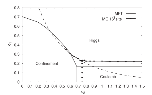
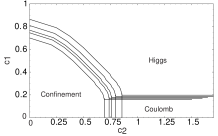
It predicts the three phases as listed in Table 1. In Fig.1 we plot the phase boundaries determined by MFT in the $c_{2}-c_{1}$ plane.

phase	$\langle U_{x\mu}\rangle_{0}$	$\langle S_{x}\rangle_{0}$	ability
Higgs	$\neq 0$	$\neq 0$	learning and recalling
Coulomb	$\neq 0$	$0$	learning
Confinement	$0$	$0$	N.A.

Table1. Three phases predicted in MFT and the associated ability of neural net in a process of learning a pattern of $S_{x}$ and retrieving it[12].

3.2 MFT for a random system

For the case of random system that involves quenched averages like (2.10), one should generalize the MFT (3.3) for a pure system. Below we develop such a generalization. For this purpose we start with the following variational system, which is independent of differences among samples;

$$Z_{0}(a) = \sum_{S_{x}}\sum_{U_{x\mu}}\exp[A_{0}(S,U,a)]\equiv\exp[-F_{0}(a)],$$

$$A_{0}(S,U,a) = \sum_{x}a_{0x}S_{x}+\sum_{x}\sum_{\mu}a_{1x\mu}U_{x\mu},$$ (3.7)

where $a_{0x}$ and $a_{1x\mu}$ are local variational parameters on the site $x$ and link $(x,x+\mu)$ respectively. (We assign the suffices 0, 1, and 2 for site, link, and plaquette objects respectively.) By applying the inequality (3.3), one has

$$F_{i}(c)\leq F_{v}(a,c)\equiv F_{0}(a)+\langle A_{0}\rangle_{0}(a)-\langle A\rangle_{0}(a,c).$$ (3.8)

By multiplying $\rho_{12}(c)$ both sides and integrating over $c_{1x\mu},c_{2x\mu\nu}$ one obtains the inequality for the free energy $F$,

$$F\leq\int[dc_{1}][dc_{2}]\rho_{12}(c)F_{v}(a,c).$$ (3.9)

Below we treat $a_{0x}$ and $a_{1x\mu}$ as random variables described by the probability distribution $\rho_{01}(a)$ defined as

$$\rho_{01}(a)=\prod_{x}[(1-q_{0})\delta(a_{0x}-a_{0})+q_{0}\delta(a_{0x}+a_{0})]\prod_{x,\mu}[(1-q_{1})\delta(a_{1x\mu}-a_{1})+q_{1}\delta(a_{1x\mu}+a_{1})],$$ (3.10)

We consider the sample average of a function $f(a)$ over samples of variational systems, each of which has different set of $a_{0x},a_{1x\mu}$, and write it as $\widetilde{f(a)}$,

$$\widetilde{f(a)}\equiv\int[da_{0}][da_{1}]\rho_{01}(a)f(a).$$ (3.11)

By multiplying $\rho_{01}(a)$ both sides of (3.9) and integrating over $a_{0x},a_{1x\mu}$, one has an upperbound $\widetilde{\overline{F}}_{v}$ for the free energy $F$ as

$$F\leq\widetilde{\overline{F}}_{v}\equiv\int[da_{0}][da_{1}][dc_{1}][dc_{2}]\rho_{01}(a)\rho_{12}(c)F_{v}(a,c).$$ (3.12)

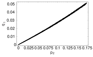
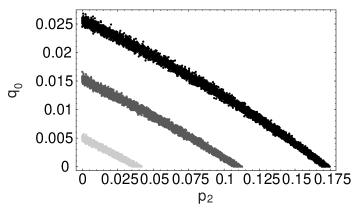
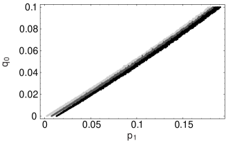
To relate $p_{1},p_{2}$ and $q_{0},q_{1}$ we regard $q_{0},q_{1}$ as concentrations of effective impurities on the sites and links respectively, and compose real impurities as the products of them. Explicitly, we determine the two functions $q_{0}(p_{1},p_{2})$ and $q_{1}(p_{1},p_{2})$ so that the following relations hold in average over samples with $\rho_{01}(a)$;

$$(1) {\rm average\ number\ of\ links\ for\ which\ sign}[a_{0x}a_{1x\mu}a_{0,x+\mu}]=-1\ {\rm is}\ 3Vp_{1}$$

$$(2) {\rm average\ number\ of\ plaquettes\ for\ which\ sign}[a_{1x\nu}a_{1,x+\nu,\mu}a_{1,x+\mu,\nu}a_{1x\mu}]=-1\ {\rm is}\ 3Vp_{2}.$$ (3.13)

In Fig.2 we present $q_{1,2}(p_{1},p_{2})$ calculated by using a 3D lattice of the size $24^{3}$.

Then $\widetilde{\overline{F}}_{v}$ of (3.12) is calculable because $\int[da_{0}][da_{1}]$ and $\int[dc_{0}][dc_{1}]$ are straightforward due to the decoupled nature of $F_{0}$, $A_{0}$ and $A$.

$$\widetilde{\overline{F}}_{v}/V = -\log[2\cosh(a_{0})]-d\log[2\cosh(a_{1})]+a_{0}\tanh(a_{0})+da_{1}\tanh(a_{1})$$ (3.14)

$$-d(1-2p_{0})(1-2q_{0})^{2}(1-2q_{1})c_{1}\tanh^{2}(a_{0})\tanh(a_{1})$$

$$-\frac{d(d-1)}{2}(1-2p_{1})(1-2q_{1})^{4}c_{2}\tanh^{4}(a_{1}).$$

$\widetilde{\overline{F}}_{v}$ becomes a function of two parameters $a_{0},a_{1}$, which we adjust to minimize it. It is straightforward to see that the conditions of minimization take the same form as the conditions (3.6) for the pure system ($p_{1}=p_{2}=0$); the former is given from the latter (the pure system) with the replacements

$$c_{1} \rightarrow c_{1}^{\prime}\equiv G_{1}(p_{1},p_{2})c_{1},$$

$$c_{2} \rightarrow c_{2}^{\prime}\equiv G_{2}(p_{1},p_{2})c_{2},$$

$$G_{1}(p_{1},p_{2}) \equiv (1-2p_{1})[1-2q_{0}(p_{1},p_{2})]^{2}[1-2q_{1}(p_{1},p_{2})],$$

$$G_{2}(p_{1},p_{2}) \equiv (1-2p_{2})[1-2q_{1}(p_{1},p_{2})]^{4}$$ (3.15)

Thus the phase transition points $(c_{1}^{\rm random},c_{2}^{\rm random})$ of the random system ($p_{1},p_{2}\neq 0$) are obatined by using the transitoin points $(c_{1}^{\rm pure},c_{2}^{\rm pure})$ of the pure system ($p_{1}=p_{2}=0$) as

$$c_{1}^{\rm random}(p_{1},p_{2}) = \frac{1}{G_{1}(p_{1},p_{2})}c_{1}^{\rm pure}$$

$$c_{2}^{\rm random}(p_{1},p_{2}) = \frac{1}{G_{2}(p_{1},p_{2})}c_{2}^{\rm pure}.$$ (3.16)

Because $G_{1,2}(p_{1},p_{2})\geq 1$, one obtains the following general inequalities

$$c_{1}^{\rm random}(p_{1},p_{2})\geq c_{1}^{\rm pure},\ \ c_{2}^{\rm random}(p_{1},p_{2})\geq c_{2}^{\rm pure}.$$ (3.17)

This implies that the effect of impurities/disorder increases the critical coupling constants, which accords with our intuition. In Fig.3 we plot the critical lines of the present model in the $c_{2}-c_{1}$ plane obtained by (3.16) for the cases of $p\ (\equiv p_{1}=p_{2})=0.015\sim 0.050$ together with the critical lines for $p=0$.

We note that the present MFT can be applied for a random lattice system similar to the present one as long as its variational free energy is decoupled to single-site and single-link integrals like (3.7). In particluar, the probability distributions $q_{0,1}(p_{1},p_{2})$ of effective impurities are universal, i.e., independent of each model, and determined by (3.13). Therefore, for each critical point of the pure system, there may be one associated critial point of the random system as a modulation due to randomness like (2.8).

4 Monte Carlo Simulations

In this section, we start with summerize the known results for $p_{1}=p_{2}=0$ and for $c_{1}=0$. Then we study the phase struture of the 3D Z(2) random Higgs lattice gauge theory by MC simulations for the case $p_{1}=p_{2}\equiv p$.

4.1 The case of $p=0$

Let us first summerize the phase structure for the pure case $p=0$. The points in Fig.1 is the phase boundary in the $c_{2}-c_{1}$ plane [6], exhibiting three phases.

The confinement-Higgs transition is first-order and terminates near $(c_{2},c_{1})\simeq(0.55,0.35)$ as the complementarity argument predicts.[17] In fact, at $c_{2}=0$, the partition function is exactly calculable by the single-link sum over $U_{x\mu}$ as

$$Z|_{c_{2}=0}=[2\cosh(c_{1})]^{3N},$$ (4.1)

which has no singularity in the $c_{1}$-dependence and so there is no phase transition along $c_{2}=0$. The Coulomb-Higgs transition is second order. In the limit $c_{2}\rightarrow\infty$, $U_{x\mu}$ becomes a pure-gauge configuration, $U_{x\mu}=W_{x+\mu}W_{x}\ (W_{x}=\pm 1)$, the system reduces to the 3D Ising spin model $A=c_{1}\sum_{x,\mu}S^{\prime}_{x+\mu}S^{\prime}_{x}\ (S^{\prime}_{x}=W_{x}S_{x})$, which exhibit a second-order phase transition at $c_{1}\simeq 0.22$. The confinement-Coulomb transition is also second order. Along $c_{1}=0$, the system reduces to the pure gauge model, which is known to exhibit a second-order phase transition at $c_{2}\simeq 0.76$.

4.2 The case of $c_{1}=0$

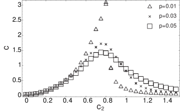
Next, let us summerize the case of no Higgs coupling ($c_{1}=0$) but with randomness. In Fig.4 we present the phase diagram in the $p-T$ ($p\equiv p_{2},\ T\equiv c_{2}^{-1}$) plane obtained in Ref.[5]. At $p=0$, a second-order phase transition at the critical point $T=T_{c}\simeq 1/0.76$. For $T<T_{c}$ the gauge-field fluctuations are small and the system is in the ordered Coulomb phase, while for $T_{c}<T$, the fluctuations are large and the system is in the disordered confinement phase. As $p$ increases from $p=0$, the critical coupling constant $T_{c}(p)$ decreases due to the randomness in gauge couplings, and it shall vanishes at a certain value $p_{0}$, $T_{c}(p_{0})=0$. The data of specific heat suggests that the order of transition changes from second order to higher order for $T$ smaller than about 1.15. $T_{c}(p)$ seems to show a “reentrance behavior”, i.e., as $T$ is lowered, the value of $p$ on the curve $T_{c}(p)$ increases first and takes the maximum value $p_{\rm max}\simeq 0.033$[5] around $T\simeq 0.4\sim 0.5$ and then decreases to end up with $p\simeq 0.029$ at $T=0$[4].

4.3 Set up of MC simulations and the global phase structure

In our MC simulations we use the standard Metropolis algorithm[18]. The typical number of sweeps in a single run for $\langle O\rangle_{i}$ of each sample is $\sim 2\times 10^{5}$. To estimate the error of $\langle O\rangle_{i}$, which we call the MC error, we divide a run into 10 successive intervals to generate 10 data. AS the MC error we estimate the standard deviation of these 10 data. The average acceptance ratios are $0.4\sim 0.5$. In Fig.5a we present a typical result of the specific heat $C$ together with the MC errors. For a random system one may be interested in the standarde deviation over samples (SDS), which should converge to a nonvanishing value even in the limit $N_{s}\rightarrow\infty$. In Fig.5b we present such SDS for the same $C$ as Fig.5a with the sample number $N_{s}=40$. By comparing these two figures, both quantities are similar in magnitude (they differ by up to factor $\sim 2$), and have similar behaviors (i.e., the $c_{1}$ dependence). In the figures below the error bars show SDS.

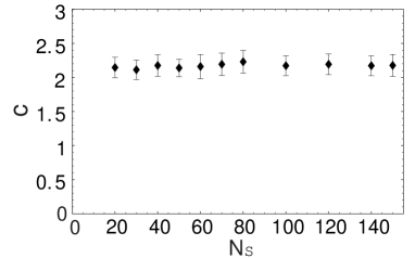
To see the dependence of $\bar{\langle O\rangle}$ on $N_{s}$ and to find a suitable value of $N_{s}$ we present in Fig.6 the specific heat $C$ vs $N_{s}$. It shows that the $N_{S}$ dependence is rather weak for $N_{S}\geq 20$. Below we show the results for $N_{s}=40$ otherwise stated, where the error bars in the figures show SDS.

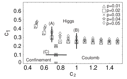
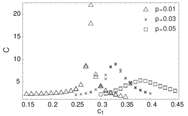
Let us first observe how the peak of the specific heat shifts as $p$ increases. In Fig.7a we present the curves of the peak location of specific heat in the $c_{2}-c_{1}$ plane. In Fig.7b, we present the specific heat for various $p$ at $c_{2}=1.0$. As $p$ increases, its peak becoms rounder and its position shifts to larger $c_{1}$ direction. It is consistent with the MFT prediction of Fig.3 in Sect.3. In Fig.7c, we present the specific heat for various $p$ at $c_{1}=0.1$. Its peak becomes rounder but its position is almost unchanged. We shall discuss the new behavior of $C$ appearing in larger latice systems.

4.4 Study of the three cases

Let us see whether these specific-heat peaks exhibit genuine phase transitions or not. To be specific, we focus on the following three cases:
(A) The confinement-Higgs transition along $c_{2}=0.7$,
(B) The Coulomb-Higgs transition along $c_{2}=1.0$,
(C) The confinement-Coulomb transition along $c_{1}=0.1$.

(A) $c_{2}=0.7$:

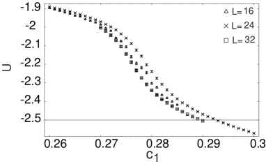
For $p=0$ we know that this case gives rise to a first-order phase transition. In Fig.8, we present $U$ and $C$ for $p=0.01$. $U$ shows no hysteresis and the peak of $C$ shows no systematic system-size dependence, which imply that this peak implies a higher-order transition or a crossover but not a first-order nor second-order phase transition. The small rendomness of $p=0.01$ is sufficient to destroy the first-order transtion of $p=0$ here. Because the firsr-order transition line for $p=0$ ends at $c_{2}\simeq 0.55$ and no phase transitions follow in the smaller $c_{2}$ region (see eq.(4.1)) it is quite possible that there are no genuine phase transitions of finite order in the case (A) for $p\geq 0.01$.

(B) $c_{2}=1.0$:

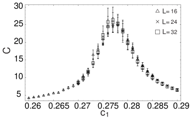
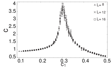
For $p=0$ this case gives rise to a second-order phase transition (See Fig.1). For $p=0.01,0.02,0.03,0.04$ the specific hear shows systematic size-dependent development, which supports that the second-order transition survives up to $p=0.04$. The peak of $C$ for $p=0.05$ fails to show systematic size dependent development. In Fig.9a,b, we compare $C$ for $p=0.04$ and $p=0.05$. Even for the size up to $L=16$, the difference appears clearly. To confirm the existence of second-order transition for $p=0.04$, we fit $C$ of $p=0.04$ with $L=24,28,32$ shown in Fig.9a by the finite-size scaling hypothesis[20] which reads for $C$ as

$$C(c_{1},L)=L^{\frac{\sigma}{\nu}}\ f(L^{\frac{1}{\nu}}\epsilon),\ \ \ \epsilon\equiv\frac{c_{1}-c_{1\infty}}{c_{1\infty}},$$ (4.2)

where $f(x)$ is the scaling function, $c_{1\infty}$ is the critical value of $c_{1}$ for the infinite system $L=\infty$, and $\sigma,\ \nu$ are the critical exponents. In Fig.9b we present $f(x)$ calculated with the choice

$$c_{1\infty}=0.277,\ \nu=0.90,\ \sigma=0.273,$$ (4.3)

which supports the existence of $f(x)$. For $p=0.05$ such a fit was impossible due to the lack of systematic size dependence.

(C) $c_{1}=0.1$:

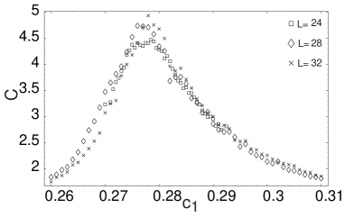
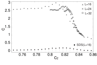
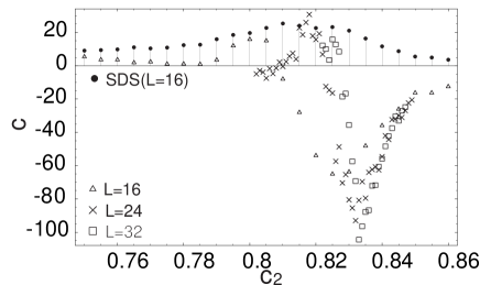
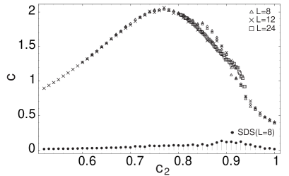
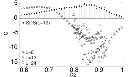
For $p=0$ we know that this case gives rise to a second-order phase transition (See Fig.1). We shall argue that this transition changes to a third-order one for $p=0.01$ and becomes a higher-order one or a cross over for $p=0.02$. In Fig.10a we present a close up of $C$ near $c_{2}=0.80$ for $p=0.01$. It shows that a small peak is developed, which shifts, as $L$ increases, to larger $c_{2}$ direction and diminishes gradually. We interprete this behavior of $C$ implies that the system is just in the transient point from the second-order transition to a higher-order one or to a crossover. We remember that the possibility of similar change from a second-order transition to a higher-order one has been pointed out in Ref.[5] for $c_{1}=0$ as one lowers the critical value of $c_{2}^{-1}$ (See Fig.4). To study this point in detail, we measured a new observable, the derivative $dC/dT$ of $C$. To introduce the “temperature” $T$ we multiply the action by a factor $\beta\equiv T^{-1}$ and making the derivative of $C$ w.r.t. $T$,

$$\frac{dC}{dT}={\rm Sample\ average\ of\ }\Big{[}-\beta^{4}\big{(}\langle A^{3}\rangle-\langle A\rangle^{3}\big{)}+\beta^{3}\big{(}\langle A^{2}\rangle-\langle A\rangle^{2}\big{)}\big{(}3\beta\langle A\rangle-2\big{)}\Big{]}/V,$$ (4.4)

and set $\beta=1$ finally. In Fig.10b we present $dC/dT$. Its signature changes at $c_{2}\simeq 0.83(L=32)$ where the small peak locates. This may be a precursor of a third-order transition. It is natural that this small peak disappears at $L\rightarrow\infty$ and a sharp edge(cliff) remains, which implies a thrid-order transition characterized by a finite gap $\Delta(dC/dT)\neq 0$. In Figs.10c,d we present $C$ and $dC/dT$ for $p=0.02$. There are no indications of possible third-order transition. They may describe a smoother transition or a crossover. The detailed study is necessary to calculate $p_{c}$ of the present case, which may involve third-order or higher-order phase transition. As explained above, this is consistent with the result of Ref.[5].

5 Conclusion and Discussion

In this paper, we considered the 3D random Z(2) Higgs lattice gauge theory and studied its global phase structure in the $c_{2}-c_{1}$ plane by a new MFT and MC simulations. The MC simulations showed that, for the case (A) of confinement-Higgs transition, the first-order transition for $p=0$ disappears quickly at $p=0.01$. For the case (B) of Coulomb-Higgs transition, the second-order transition for $p=0$ persists up to $p=0.04$. The result for $p=0.05$ is failed to fit the scaling law. For the case (C) of confinement-Coulomb transition, as $L$ increases, a small peak in $C$ developes for $p=0.01$ and then diminishes, which leads to a third-order transition. However, for $p=0.02$, a third-order transition has not been observed, so further study is necessary to explore a possible higher-order transition.

Let us discuss some implications of these results for a quantum memory. Inclusion of the Higgs coupling produces the third Higgs phase which has the least fluctuations of variables among the three phases, and so more stable functions than in the Coulomb phase are expected. The estimated critical concentration $p_{c}\simeq 0.04\sim 0.05$ for the case (B) is larger than $p_{c}\simeq 0.033$ for $c_{1}=0$. Of course, the nonlocal observables become more complicated than the Wilson loop itself[9].

Concerning to the neural network, “thermal” fluctuations previously considered as noise effects in Ref.[6, 12] act uniformly in space. In contrast, the random effects considered in the present model are inhomogeneous. However, these two effects seem to have no crucial qualitative differences for a system staying near a phase boundary but just inside the Higgs phase. Either introduction of tiny amount ofrandomnessin the local coupling constants or heating the sytem by tiny amount of temperature rise necessarily drives the system into the Coulomb or confinement phase.

When one tries to include the time evolution to a 3D neural net in a manner faithful to quantum theory and/or statistical mechanics, one faces a 4D system (with the imaginary-time as the fourth direction). Then the effect of randomness to such a 4D system in of interest. Some analyses have appeared for 4D Z(2) RPGM[21]. Including the Higgs coupling to this 4D model may be an interesting subject to study.

Figure 1: Phase diagram by MFT for $p=0$. The dots represents the results of MC simulations.[6] The dashed curve $c_{2}=-\frac{1}{2}{\rm\ell nth}(c_{1})$ is the exact results obtianed by the self-duality argument[16], on which some of the transition points may lie.

(a)                                             (b)

                          (c)                                             (d)

Figure 2: $q_{0}(p_{1},p_{2})$ and $q_{1}(p_{1},p_{2})$ satisfying (3.13) calculated by using a 3D lattice of the size $24^{3}$. (a) $p_{2}$ vs $q_{1}$ for $p_{1}=0.01,0.03,0.05$. $q_{1}$ is independent of $p_{1}$ because the wrong $p_{2}$-plaquettes are generated by $q_{1}$-links alone without $q_{0}$-sites. (b) $p_{2}$ vs $q_{0}$ for $p_{1}=0.01,0.03,0.05$ from below. $q_{0}$ decreases as $p_{2}$ increases because too sufficient number of $q_{1}$-links are generated to make $p_{2}$-plaquettes. (c) $p_{1}$ vs $q_{1}$ for $p_{2}=0.01,0.03,0.05$ from below. $q_{1}$ is independent of $p_{1}$ because $q_{1}$ is fixed only by the number of $p_{2}$-plaquettes. (d) $p_{1}$ vs $q_{0}$ for $p_{2}=0.01,0.03,0.05$ from above. For very small $p_{1}$, $q_{0}$-sites are unnecessary because of sufficient $q_{1}$-links supplied to compose $p_{2}$-plaquettes.

Figure 3: The phase diagram in the $c_{2}-c_{1}$ plane determined by the mean-field theory for $p=0,0.015,0.022,0.035,0.05$ from below. As the disorder increases, the region of Higgs phase diminishes.

Figure 4: Phase diagram in the $p-T$ ($p=p_{2},T=c_{2}^{-1}$) plane for $c_{1}=0$ from Ref.[5]. The phase boundary $p=p_{c}(T)$ gives the maximum value $p\simeq 0.0332\sim 0.033$ at $T\simeq 0.3\sim 0.4$. It ends at $T=0$ with $p\simeq 0.029$[4]. The solid curve is the Nishimori line[19] on which the “thermal” effects valances with the “random” effects.

(a)                                             (b)

Figure 5: Specific heat for $c_{2}=1.0$ and $p=0.04$ with $L=24$, $N_{s}=40$. (a) With MC errors and (b) With standard deviation over samples (SDS).

Figure 6: Sample number ($N_{s}$) dependence of the specific heat for $c_{2}=1.0,c_{1}=0.27$ with $p=0.03$ and $L=12$ with SDS.

(a)


                          (b)                                             (c)

Figure 7: (a) Phase diagram in the $c_{2}-c_{1}$ plane with the possible phase boundary curves determined by the location of the peak of specific heat $C$ with $L=12$. The three segments marked by (A,B,C) show the cases we shall examine in detail below. (b) $p$-dependence of the specific heat $C$ for $c_{2}=1.0$ with $L=12$. (c) $p$-dependence of the specific heat $C$ for $c_{1}=0.1$ with $L=12$.

(a)                                                      (b)

Figure 8: Inernal energy $U$ and the specific heat $C$ for the case (A) $c_{2}=0.7$ at $p=0.01$. (a) $U$ has no hysteresis and (b) $C$ has no systematic size dependence.

(a)                                                              (b)


                          (c)                                                              (d)

Figure 9: Specific heat $C$ for the case (B) $c_{2}=1.0$. (a) $C$ for $p=0.04$; (b) $C$ for $p=0.05$. (c) $C$ for $p=0.04$ before scaling; (d) $C$ for $p=0.04$ after scaling.

(a)                                                              (b)


                                   (c)                                                              (d)

Figure 10: $C$ and $dC/dT$ for the case (C) $c_{1}=0.1$. (a) $C$ for $p=0.01$, (b) $dC/dT$ for $p=0.01$, (c) $C$ for $p=0.02$, (d) $dC/dT$ for $p=0.02$. In each figure the SDS are shown separately.

References

- [1] P. W. Anderson, Phys. Rev.109,1492(1958).
- [2] A. Yu. Kitaev, in Proceedings of the Third International Conference on Quantum Communication and Measurement, ed. O. Hirota, A. S. Holevo, and C. M. Caves (New York, Plenum, 1997); Annals Phys.303, 2(2003).
- [3] J. Preskill, in “Introduction to Quantum Computation”, ed. H. K. Lo, S. Popescu and T. P. Spiller (World Scientific, 1998), quant-ph/9712048; E. Dennis, A. Kitaev, A. Landahl, and J. Preskill, J.Math.Phys.43, 4452 (2002); C. Mochon, Phys.Rev.A67, 022315(2003); G. Arakawa and I. Ichinose, Annals Phys.311, 152(2004); K. Takeda and H. Nishimori, Nucl. Phys. B686 (2004) 377.
- [4] C. Wang, J. Harrington and J. Preskill, Annals Phys. 303, 31 (2003).
- [5] T. Ohno, G. Arakawa, I. Ichinose, T. Matsui, Nucl. Phys. B697,462(2004).
- [6] M.Kemuriyama, T.Matsui and K.Sakakibara, Physica A356, 525-553(2005).
- [7] See, e.g., P. A. Lee, N. Nagaosa, and X.-G. Wen, Rev. Mod. Phys.78, 17 (2006); I.Ichinose, T.Matsui and M.Onoda, Phys. Rev. B64, 104516(1-22) (2001).
- [8] S. Takashima, I.Ichinose, and T. Matsui, Phys. Rev. B72,075112(1-16)(2005).
- [9] K. Fredenhagen and M. Marcu, Commun Math. Phys. 92,81(1983); J. Bricmont and J. Froehlich, Phys.Lett. B122,73(1983).
- [10] S. Haykin, “Neural Networks; A Comprehensive Foundation”, Macmillan Pub. Co., 1994.
- [11] J.J. Hopfield, Proc.Natl.Acad.Sci. USA 79,2554(1982).
- [12] T.Matsui, ”Gauge Symmetry and Neural Networks”, cond-mat/0112463, pp. 271-280 in ”Fluctuating Paths and Fields”, ed. by W.Janke et al., World Scientific (2001); Y.Fujita and T.Matsui, cond-mat/0207023, Proceedings of 9th International Conference on Neural Information Processing, ed. by L.Wang et al., 1360-1367(2002).
- [13] R. P. Feynman, ”Statistical Mechanics, A set of Lectures”, Chap.8, W. A. Benjamin (1972).
- [14] S. Elitzur, Phys. Rev.D12, 3978 (1975).
- [15] J. M. Drouffe, Nucl. Phys.B170, 211 (1980).
- [16] F.Wegner, J.Math.Phys.12, 2259 (1971).
- [17] E.Fradkin and S.Shenker, Phys.Rev.D19,3682(1979).
- [18] N. Metropolis, A. W. Rosenbluth, M. N. Rosenbluth, A. M. Teller, E. Teller, J. Chem. Phys.21,1087(1953).
- [19] H. Nishimori, Prog. Theor. Phys.66, 1169 (1981).
- [20] C. Domb and M. S. Green, eds., “Phase Transition and Critical Phenomena”, vol.6. Academic Press, New York, 1976.
- [21] K. Takeda and H. Nishimori, Nucl. Phys. B 686 (2004) 377; G. Arakawa, I. Ichinose, T. Matsui, K. Takeda, Nucl. Phys. B709, 296 (2005).