Domain decomposition methods for compressed sensing

Massimo Fornasier Johann Radon Institute for Computational and Applied Mathematics (RICAM), Austrian Academy of Sciences, Altenbergerstrasse 69, A-4040, Linz, Austria Email: massimo.fornasier@oeaw.ac.at    Andreas Langer Johann Radon Institute for Computational and Applied Mathematics (RICAM), Austrian Academy of Sciences, Altenbergerstrasse 69, A-4040, Linz, Austria Email: andreas.langer@oeaw.ac.at    Carola-Bibiane Schönlieb Department of Applied Mathematics and Theoretical Physics (DAMTP), Centre for Mathematical Sciences, Wilberforce Road, Cambridge CB3 0WA, United Kingdom.Email: c.b.s.schonlieb@damtp.cam.ac.uk
Abstract

We present several domain decomposition algorithms for sequential and parallel minimization of functionals formed by a discrepancy term with respect to data and total variation constraints. The convergence properties of the algorithms are analyzed. We provide several numerical experiments, showing the successful application of the algorithms for the restoration 1D and 2D signals in interpolation/inpainting problems respectively, and in a compressed sensing problem, for recovering piecewise constant medical-type images from partial Fourier ensembles.

1 Introduction

In concrete applications for image processing, one might be interested to recover at best a digital image provided only partial linear or nonlinear measurements, possibly corrupted by noise. Given the observation that natural and man-made images are characterized by a relatively small number of edges and extensive relatively uniform parts, one may want to help the reconstruction by imposing that the interesting solution is the one which matches the given data and has also a few discontinuities localized on sets of lower dimension.

In the context of compressed sensing [2, 8], it has been clarified the fundamental role of minimizing 1subscript1\ell_{1}-norms in order to promote sparse solutions. This understanding furnishes an important interpretation of total variation minimization, i.e., the minimization of the 1subscript1\ell_{1}-norm of derivatives [13], as a regularization technique for image restoration. Several numerical strategies to perform efficiently total variation minimization have been proposed in the literature. We list a few of the relevant ones, ordered by their chronological appearance:

(i) the approach of Chambolle and Lions [4] by re-weighted least squares, see also [6] for generalizations and refinements in the context of compressed sensing;

(ii) variational approximation via local quadratic functionals as in the work of Vese et al. [14, 1];

(iii) iterative thresholding algorithms based on projections onto convex sets as in the work of Chambolle [3] as well as in the work of Combettes-Wajs [5] and Daubechies et al. [7];

(iv) iterative minimization of the Bregman distance as in the work of Osher et al. [12];

(v) the approach proposed by Nesterov [11] and its modifications by Weiss et al. [15].

These approaches differ significantly, and it seems that the ones collected in the groups iv) and v) do show presently the best performances in practice. However, none of the mentioned methods is able to address in real-time, or at least in an acceptable computational time, extremely large problems, such as 4D imaging (spatial plus temporal dimensions) from functional magnetic-resonance in nuclear medical imaging, astronomical imaging or global terrestrial seismic tomography. For such large scale simulations we need to address methods which allow us to reduce the problem to a finite sequence of sub-problems of more manageable size, perhaps by one of the methods listed above. With this aim we introduced subspace correction and domain decomposition methods both for 1subscript1\ell_{1}-norm and total variation minimizations [9, 10]. Due to the nonadditivity of the total variation with respect to a domain decomposition (the total variation of a function on the whole domain equals the sum of the total variations on the subdomains plus the size of the jumps at the interfaces), one encounters additional difficulties in showing convergence of such decomposition strategies to global minimizers.

In this paper we review concisely both nonoverlapping and overlapping domain decomposition methods for total variation minimization and we provide their properties of convergence to global minimizers. Moreover, we show numerical applications in classical problems of signal and image processing, such as signal interpolation and image inpainting. We further include applications in the context of compressed sensing for recovering piecewise constant medical-type images from partial Fourier ensembles [2].

2 Notations and preliminaries

Since we are interested to a discrete setting, we define the domain of our multivariate digital signal Ω={x11<<xN11}××{x1d<<xNdd}dΩsuperscriptsubscript𝑥11superscriptsubscript𝑥subscript𝑁11superscriptsubscript𝑥1𝑑superscriptsubscript𝑥subscript𝑁𝑑𝑑superscript𝑑\Omega=\{x_{1}^{1}<\ldots<x_{N_{1}}^{1}\}\times\ldots\times\{x_{1}^{d}<\ldots<x_{N_{d}}^{d}\}\subset\mathbb{R}^{d}, d𝑑d\in\mathbb{N} and we consider the signal space =N1×N2××Ndsuperscriptsubscript𝑁1subscript𝑁2subscript𝑁𝑑\mathcal{H}=\mathbb{R}^{N_{1}\times N_{2}\times\ldots\times N_{d}}, where Nisubscript𝑁𝑖N_{i}\in\mathbb{N} for i=1,,d𝑖1𝑑i=1,\ldots,d. For u𝑢u\in\mathcal{H} we write u=u(x𝐢)𝐢𝑢𝑢subscriptsubscript𝑥𝐢𝐢u=u(x_{\mathbf{i}})_{\mathbf{i}\in\mathcal{I}} with index set :=k=1d{1,,Nk}assignsuperscriptsubscriptproduct𝑘1𝑑1subscript𝑁𝑘\mathcal{I}:=\prod_{k=1}^{d}\{1,\ldots,N_{k}\} and u(x𝐢)=u(xi11,,xidd)𝑢subscript𝑥𝐢𝑢superscriptsubscript𝑥subscript𝑖11superscriptsubscript𝑥subscript𝑖𝑑𝑑u(x_{\mathbf{i}})=u(x_{i_{1}}^{1},\ldots,x_{i_{d}}^{d}) where ik{1,,Nk}subscript𝑖𝑘1subscript𝑁𝑘i_{k}\in\{1,\ldots,N_{k}\} and x𝐢Ωsubscript𝑥𝐢Ωx_{\mathbf{i}}\in\Omega. Then, for gN𝑔superscript𝑁g\in\mathbb{R}^{N}, the psubscript𝑝\ell_{p}-norm is given by gp=(k=1N|gk|p)1/p,1p<formulae-sequencesubscriptnorm𝑔𝑝superscriptsuperscriptsubscript𝑘1𝑁superscriptsubscript𝑔𝑘𝑝1𝑝1𝑝\|g\|_{p}=\left(\sum_{k=1}^{N}|g_{k}|^{p}\right)^{1/p},\quad 1\leq p<\infty, and for u𝑢u\in\mathcal{H} the discrete gradient u𝑢\nabla u is given by (u)(x𝐢)=((u)1(x𝐢),,(u)d(x𝐢))𝑢subscript𝑥𝐢superscript𝑢1subscript𝑥𝐢superscript𝑢𝑑subscript𝑥𝐢(\nabla u)(x_{\mathbf{i}})=((\nabla u)^{1}(x_{\mathbf{i}}),\ldots,(\nabla u)^{d}(x_{\mathbf{i}})) with (u)j(x𝐢)=u(xi11,,xij+1j,,xidd)u(xi11,,xijj,,xidd)superscript𝑢𝑗subscript𝑥𝐢𝑢subscriptsuperscript𝑥1subscript𝑖1subscriptsuperscript𝑥𝑗subscript𝑖𝑗1subscriptsuperscript𝑥𝑑subscript𝑖𝑑𝑢subscriptsuperscript𝑥1subscript𝑖1subscriptsuperscript𝑥𝑗subscript𝑖𝑗subscriptsuperscript𝑥𝑑subscript𝑖𝑑(\nabla u)^{j}(x_{\mathbf{i}})=u(x^{1}_{i_{1}},\ldots,x^{j}_{i_{j}+1},\ldots,x^{d}_{i_{d}})-u(x^{1}_{i_{1}},\ldots,x^{j}_{i_{j}},\ldots,x^{d}_{i_{d}}) if ij<Njsubscript𝑖𝑗subscript𝑁𝑗i_{j}<N_{j}, and (u)j(x𝐢)=0superscript𝑢𝑗subscript𝑥𝐢0(\nabla u)^{j}(x_{\mathbf{i}})=0 if ij=Njsubscript𝑖𝑗subscript𝑁𝑗i_{j}=N_{j}, for all j=1,,d𝑗1𝑑j=1,\ldots,d and for all 𝐢=(i1,,id)𝐢subscript𝑖1subscript𝑖𝑑\mathbf{i}=(i_{1},\ldots,i_{d})\in\mathcal{I}. The total variation of u𝑢u\in\mathcal{H} in the discrete setting is then defined as |D(u)|(Ω)=𝐢|(u)(x𝐢)|𝐷𝑢Ωsubscript𝐢𝑢subscript𝑥𝐢\left|D(u)\right|(\Omega)=\sum\limits_{\mathbf{i}\in\mathcal{I}}\left|(\nabla u)(x_{\mathbf{i}})\right|, with |y|=y12++yd2𝑦superscriptsubscript𝑦12superscriptsubscript𝑦𝑑2|y|=\sqrt{y_{1}^{2}+\ldots+y_{d}^{2}} for every y=(y1,,yd)d𝑦subscript𝑦1subscript𝑦𝑑superscript𝑑y=(y_{1},\ldots,y_{d})\in\mathbb{R}^{d}. We define the scalar product of u,v𝑢𝑣u,v\in\mathcal{H} as usual, u,v=𝐢u(x𝐢)v(x𝐢)subscript𝑢𝑣subscript𝐢𝑢subscript𝑥𝐢𝑣subscript𝑥𝐢\langle u,v\rangle_{\mathcal{H}}=\sum_{\mathbf{i}\in\mathcal{I}}u(x_{\mathbf{i}})v(x_{\mathbf{i}}), and the scalar product of p,qd𝑝𝑞superscript𝑑p,q\in\mathcal{H}^{d} as p,qd=𝐢p1(x𝐢)q1(x𝐢)++pd(x𝐢)qd(x𝐢)subscript𝑝𝑞superscript𝑑subscript𝐢superscript𝑝1subscript𝑥𝐢superscript𝑞1subscript𝑥𝐢superscript𝑝𝑑subscript𝑥𝐢superscript𝑞𝑑subscript𝑥𝐢\langle p,q\rangle_{\mathcal{H}^{d}}=\sum_{\mathbf{i}\in\mathcal{I}}p^{1}(x_{\mathbf{i}})q^{1}(x_{\mathbf{i}})+\ldots+p^{d}(x_{\mathbf{i}})q^{d}(x_{\mathbf{i}}). Further we introduce a discrete divergence div:d:divsuperscript𝑑\operatorname{div}:\mathcal{H}^{d}\to\mathcal{H} defined, by analogy with the continuous setting, by div=divsuperscript\operatorname{div}=-\nabla^{*} (superscript\nabla^{*} is the adjoint of the gradient \nabla). In the following we denote with πKsubscript𝜋𝐾\pi_{K} the orthogonal projection onto a closed convex set K𝐾K.

2.1 Projections onto convex sets

With these notation, we define the closed convex set

K:={divp:pd,|p𝐢|1 for all 𝐢}.assign𝐾conditional-setdiv𝑝formulae-sequence𝑝superscript𝑑subscript𝑝𝐢1 for all 𝐢\displaystyle K:=\left\{\operatorname{div}p:p\in\mathcal{H}^{d},\left|p_{\mathbf{i}}\right|\leq 1\;\mbox{ for all }\mathbf{i}\in\mathcal{I}\right\}.

We briefly recall here an algorithm proposed by Chambolle in [3] in order to compute the projection onto αK𝛼𝐾\alpha K. The following semi-implicit gradient descent algorithm is given to approximate παK(g)subscript𝜋𝛼𝐾𝑔\pi_{\alpha K}(g): Choose τ>0𝜏0\tau>0, let p(0)=0superscript𝑝00p^{(0)}=0 and, for any n0𝑛0n\geq 0, iterate

p𝐢(n+1)=p𝐢(n)+τ((divp(n)g/α))𝐢1+τ|((divp(n)g/α))𝐢|.superscriptsubscript𝑝𝐢𝑛1superscriptsubscript𝑝𝐢𝑛𝜏subscriptdivsuperscript𝑝𝑛𝑔𝛼𝐢1𝜏subscriptdivsuperscript𝑝𝑛𝑔𝛼𝐢\displaystyle p_{\mathbf{i}}^{(n+1)}=\frac{p_{\mathbf{i}}^{(n)}+\tau(\nabla(\operatorname{div}p^{(n)}-g/\alpha))_{\mathbf{i}}}{1+\tau\left|(\nabla(\operatorname{div}p^{(n)}-g/\alpha))_{\mathbf{i}}\right|}. (1)

For τ>0𝜏0\tau>0 sufficiently small, the iteration αdivp(n)𝛼divsuperscript𝑝𝑛\alpha\operatorname{div}p^{(n)} converges to παK(g)subscript𝜋𝛼𝐾𝑔\pi_{\alpha K}(g) as n𝑛n\rightarrow\infty (compare [3, Theorem 3.1]).

2.2 Setting of the problem

Given a model linear operator T:K:𝑇superscript𝐾T:\mathcal{H}\to\mathbb{R}^{K}, we are considering the following discrete minimization problem

argminu{𝒥(u):=Tug22+2α|Du|(Ω)}subscript𝑢assign𝒥𝑢superscriptsubscriptnorm𝑇𝑢𝑔222𝛼𝐷𝑢Ω\arg\min_{u\in\mathcal{H}}\left\{\mathcal{J}(u):=\|Tu-g\|_{2}^{2}+2\alpha|Du|(\Omega)\right\} (2)

where gK𝑔superscript𝐾g\in\mathbb{R}^{K} is a given datum and α>0𝛼0\alpha>0 is a fixed regularization parameter. Note that, up to rescaling the parameter α𝛼\alpha and the datum g𝑔g, we can always assume T<1norm𝑇1\|T\|<1. Moreover, in order to ensure existence of solutions, we assume 1ker(T)1kernel𝑇1\notin\ker(T). For both nonoverlapping and overlapping domain decompositions, we will consider a linear sum =V1+V2subscript𝑉1subscript𝑉2\mathcal{H}=V_{1}+V_{2} with respect to two subspaces V1subscript𝑉1V_{1}, V2subscript𝑉2V_{2} defined by a suitable decomposition of the physical domain ΩΩ\Omega. We restrict our discussion to two subspaces, but the analysis can be extended in a straightforward way to multiple subspaces. With this splitting we want to minimize 𝒥𝒥\mathcal{J} by suitable instances of the following alternating algorithm: Pick an initial V1+V2u1(0)+u2(0):=u(0)containssubscript𝑉1subscript𝑉2superscriptsubscript𝑢10superscriptsubscript𝑢20assignsuperscript𝑢0V_{1}+V_{2}\ni u_{1}^{(0)}+u_{2}^{(0)}:=u^{(0)}\in\mathcal{H}, for example u(0)=0superscript𝑢00u^{(0)}=0, and iterate

{u1(n+1)argminv1V1𝒥(v1+u2(n))u2(n+1)argminv2V2𝒥(u1(n+1)+v2)u(n+1):=u1(n+1)+u2(n+1).casessuperscriptsubscript𝑢1𝑛1subscriptsubscript𝑣1subscript𝑉1𝒥subscript𝑣1superscriptsubscript𝑢2𝑛missing-subexpressionsuperscriptsubscript𝑢2𝑛1subscriptsubscript𝑣2subscript𝑉2𝒥superscriptsubscript𝑢1𝑛1subscript𝑣2missing-subexpressionassignsuperscript𝑢𝑛1superscriptsubscript𝑢1𝑛1superscriptsubscript𝑢2𝑛1missing-subexpression\left\{\begin{array}[]{ll}u_{1}^{(n+1)}\approx\arg\min_{v_{1}\in V_{1}}\mathcal{J}(v_{1}+u_{2}^{(n)})&\\ u_{2}^{(n+1)}\approx\arg\min_{v_{2}\in V_{2}}\mathcal{J}(u_{1}^{(n+1)}+v_{2})&\\ u^{(n+1)}:=u_{1}^{(n+1)}+u_{2}^{(n+1)}.\end{array}\right.

3 Nonoverlapping domain decomposition methods

Let us consider the disjoint domain decomposition Ω=Ω1Ω2ΩsubscriptΩ1subscriptΩ2\Omega=\Omega_{1}\cup\Omega_{2} and Ω1Ω2=subscriptΩ1subscriptΩ2\Omega_{1}\cap\Omega_{2}=\emptyset and the corresponding spaces Vj={u:supp(u)Ωj}subscript𝑉𝑗conditional-set𝑢supp𝑢subscriptΩ𝑗V_{j}=\{u\in\mathcal{H}:\operatorname{supp}(u)\subset\Omega_{j}\}, for j=1,2𝑗12j=1,2. Note that =V1V2direct-sumsubscript𝑉1subscript𝑉2\mathcal{H}=V_{1}\oplus V_{2}. It is useful to us to introduce an auxiliary functional 𝒥1ssubscriptsuperscript𝒥𝑠1\mathcal{J}^{s}_{1}, called the surrogate functional of 𝒥𝒥\mathcal{J}: For j{1,2}𝑗12j\in\{1,2\} and jˇ{1,2}{j}ˇ𝑗12𝑗\check{j}\in\{1,2\}\setminus\{j\}, assume a,ujVj𝑎subscript𝑢𝑗subscript𝑉𝑗a,u_{j}\in V_{j} and ujˇVjˇsubscript𝑢ˇ𝑗subscript𝑉ˇ𝑗u_{\check{j}}\in V_{\check{j}} and define

𝒥js(uj+ujˇ,a):=𝒥(uj+ujˇ)+uja2T(uja)2.assignsubscriptsuperscript𝒥𝑠𝑗subscript𝑢𝑗subscript𝑢ˇ𝑗𝑎𝒥subscript𝑢𝑗subscript𝑢ˇ𝑗superscriptsubscriptnormsubscript𝑢𝑗𝑎2superscriptsubscriptnorm𝑇subscript𝑢𝑗𝑎2\mathcal{J}^{s}_{j}(u_{j}+u_{\check{j}},a):=\mathcal{J}(u_{j}+u_{\check{j}})+\|u_{j}-a\|_{\mathcal{H}}^{2}-\|T(u_{j}-a)\|_{\mathcal{H}}^{2}. (3)

As it will be clarified later, the minimization of 𝒥js(uj+ujˇ,a)subscriptsuperscript𝒥𝑠𝑗subscript𝑢𝑗subscript𝑢ˇ𝑗𝑎\mathcal{J}^{s}_{j}(u_{j}+u_{\check{j}},a) with respect to ujsubscript𝑢𝑗u_{j} and for fixed ujˇ,asubscript𝑢ˇ𝑗𝑎u_{\check{j}},a is an operation which can be realized more easily than the direct minimization of the parent functional 𝒥(uj+ujˇ)𝒥subscript𝑢𝑗subscript𝑢ˇ𝑗\mathcal{J}(u_{j}+u_{\check{j}}) for the sole ujˇsubscript𝑢ˇ𝑗u_{\check{j}} fixed.

3.1 Sequential algorithm

In the following we denote uj=πVjusubscript𝑢𝑗subscript𝜋subscript𝑉𝑗𝑢u_{j}=\pi_{V_{j}}u the orthogonal projection onto Vjsubscript𝑉𝑗V_{j}, for j=1,2𝑗12j=1,2. Let us explicitely express the algorithm as follows: Pick an initial V1V2u1(0,L)+u2(0,M):=u(0)containsdirect-sumsubscript𝑉1subscript𝑉2superscriptsubscript𝑢10𝐿superscriptsubscript𝑢20𝑀assignsuperscript𝑢0V_{1}\oplus V_{2}\ni u_{1}^{(0,L)}+u_{2}^{(0,M)}:=u^{(0)}\in\mathcal{H}, for example u(0)=0superscript𝑢00u^{(0)}=0, and iterate

{{u1(n+1,0)=u1(n,L) and for =0,,L1u1(n+1,+1)=argminu1V1𝒥1s(u1+u2(n,M),u1(n+1,)){u2(n+1,0)=u2(n,M) and for m=0,,M1u2(n+1,m+1)=argminu2V2𝒥2s(u1(n+1,L)+u2,u2(n+1,m))u(n+1):=u1(n+1,L)+u2(n+1,M).casescasesformulae-sequencesuperscriptsubscript𝑢1𝑛10superscriptsubscript𝑢1𝑛𝐿 and for 0𝐿1missing-subexpressionsuperscriptsubscript𝑢1𝑛11subscriptsubscript𝑢1subscript𝑉1superscriptsubscript𝒥1𝑠subscript𝑢1superscriptsubscript𝑢2𝑛𝑀superscriptsubscript𝑢1𝑛1missing-subexpressionmissing-subexpressioncasesformulae-sequencesuperscriptsubscript𝑢2𝑛10superscriptsubscript𝑢2𝑛𝑀 and for 𝑚0𝑀1missing-subexpressionsuperscriptsubscript𝑢2𝑛1𝑚1subscriptsubscript𝑢2subscript𝑉2superscriptsubscript𝒥2𝑠superscriptsubscript𝑢1𝑛1𝐿subscript𝑢2superscriptsubscript𝑢2𝑛1𝑚missing-subexpressionmissing-subexpressionassignsuperscript𝑢𝑛1superscriptsubscript𝑢1𝑛1𝐿superscriptsubscript𝑢2𝑛1𝑀missing-subexpression\left\{\begin{array}[]{ll}\left\{\begin{array}[]{ll}u_{1}^{(n+1,0)}=u_{1}^{(n,L)}\mbox{ and for }\ell=0,\dots,L-1&\\ u_{1}^{(n+1,\ell+1)}=\arg\min_{u_{1}\in V_{1}}\mathcal{J}_{1}^{s}(u_{1}+u_{2}^{(n,M)},u_{1}^{(n+1,\ell)})&\\ \end{array}\right.&\\ \left\{\begin{array}[]{ll}u_{2}^{(n+1,0)}=u_{2}^{(n,M)}\mbox{ and for }m=0,\dots,M-1&\\ u_{2}^{(n+1,m+1)}=\arg\min_{u_{2}\in V_{2}}\mathcal{J}_{2}^{s}(u_{1}^{(n+1,L)}+u_{2},u_{2}^{(n+1,m)})&\\ \end{array}\right.&\\ u^{(n+1)}:=u_{1}^{(n+1,L)}+u_{2}^{(n+1,M)}.\end{array}\right. (4)

Note that we do prescribe a finite number L𝐿L and M𝑀M of inner iterations for each subspace respectively.

3.2 Parallel algorithm

The parallel version of the previous algorithm reads as follows: Pick an initial V1V2u1(0,L)+u2(0,M):=u(0)containsdirect-sumsubscript𝑉1subscript𝑉2superscriptsubscript𝑢10𝐿superscriptsubscript𝑢20𝑀assignsuperscript𝑢0V_{1}\oplus V_{2}\ni u_{1}^{(0,L)}+u_{2}^{(0,M)}:=u^{(0)}\in\mathcal{H}, for example u(0)=0superscript𝑢00u^{(0)}=0, and iterate

{{u1(n+1,0)=u1(n,L) and for =0,,L1u1(n+1,+1)=argminu1V1𝒥1s(u1+u2(n,M),u1(n+1,)){u2(n+1,0)=u2(n,M) and for m=0,,M1u2(n+1,m+1)=argminu2V2𝒥2s(u1(n,L)+u2,u2(n+1,m))u(n+1):=u1(n+1,L)+u2(n+1,M)+u(n)2.casescasesformulae-sequencesuperscriptsubscript𝑢1𝑛10superscriptsubscript𝑢1𝑛𝐿 and for 0𝐿1missing-subexpressionsuperscriptsubscript𝑢1𝑛11subscriptsubscript𝑢1subscript𝑉1superscriptsubscript𝒥1𝑠subscript𝑢1superscriptsubscript𝑢2𝑛𝑀superscriptsubscript𝑢1𝑛1missing-subexpressionmissing-subexpressioncasesformulae-sequencesuperscriptsubscript𝑢2𝑛10superscriptsubscript𝑢2𝑛𝑀 and for 𝑚0𝑀1missing-subexpressionsuperscriptsubscript𝑢2𝑛1𝑚1subscriptsubscript𝑢2subscript𝑉2superscriptsubscript𝒥2𝑠superscriptsubscript𝑢1𝑛𝐿subscript𝑢2superscriptsubscript𝑢2𝑛1𝑚missing-subexpressionmissing-subexpressionassignsuperscript𝑢𝑛1superscriptsubscript𝑢1𝑛1𝐿superscriptsubscript𝑢2𝑛1𝑀superscript𝑢𝑛2missing-subexpression\left\{\begin{array}[]{ll}\left\{\begin{array}[]{ll}u_{1}^{(n+1,0)}=u_{1}^{(n,L)}\mbox{ and for }\ell=0,\dots,L-1&\\ u_{1}^{(n+1,\ell+1)}=\arg\min_{u_{1}\in V_{1}}\mathcal{J}_{1}^{s}(u_{1}+u_{2}^{(n,M)},u_{1}^{(n+1,\ell)})&\\ \end{array}\right.&\\ \left\{\begin{array}[]{ll}u_{2}^{(n+1,0)}=u_{2}^{(n,M)}\mbox{ and for }m=0,\dots,M-1&\\ u_{2}^{(n+1,m+1)}=\arg\min_{u_{2}\in V_{2}}\mathcal{J}_{2}^{s}(u_{1}^{(n,L)}+u_{2},u_{2}^{(n+1,m)})&\\ \end{array}\right.&\\ u^{(n+1)}:=\frac{u_{1}^{(n+1,L)}+u_{2}^{(n+1,M)}+u^{(n)}}{2}.\end{array}\right. (5)

Note that u(n+1)superscript𝑢𝑛1u^{(n+1)} is the average of the current iteration and the previous one as it is the case for successive overrelaxation methods (SOR) in classical numerical linear algebra.

4 Overlapping domain decomposition methods

Let us consider the overlapping domain decomposition Ω=Ω1Ω2ΩsubscriptΩ1subscriptΩ2\Omega=\Omega_{1}\cup\Omega_{2} and Ω1Ω2subscriptΩ1subscriptΩ2\Omega_{1}\cap\Omega_{2}\neq\emptyset and the corresponding spaces Vj={u:supp(u)Ωj}subscript𝑉𝑗conditional-set𝑢supp𝑢subscriptΩ𝑗V_{j}=\{u\in\mathcal{H}:\operatorname{supp}(u)\subset\Omega_{j}\}, for j=1,2𝑗12j=1,2. Note that now =V1+V2subscript𝑉1subscript𝑉2\mathcal{H}=V_{1}+V_{2} is not anymore a direct sum of V1subscript𝑉1V_{1} and V2subscript𝑉2V_{2}, but just a linear sum of subspaces. We define the internal boundaries Γj=ΩjΩjˇsubscriptΓ𝑗subscriptΩ𝑗subscriptΩˇ𝑗\Gamma_{j}=\partial\Omega_{j}\cap\Omega_{\check{j}}, j{1,2}𝑗12j\in\{1,2\} and jˇ{1,2}{j}ˇ𝑗12𝑗\check{j}\in\{1,2\}\setminus\{j\} (see Figure 1).

Ω2subscriptΩ2\Omega_{2}Γ2subscriptΓ2\Gamma_{2}Γ1subscriptΓ1\Gamma_{1}Ω1subscriptΩ1\Omega_{1}

Figure 1: Overlapping domain decomposition and internal boundaries.

4.1 Sequential algorithm

Associated to the decomposition {Ωj:j=1,2}conditional-setsubscriptΩ𝑗𝑗12\{\Omega_{j}:j=1,2\} let us fix a partition of unity {χj:j=1,2}conditional-setsubscript𝜒𝑗𝑗12\{\chi_{j}:j=1,2\}, i.e., χ1+χ2=1subscript𝜒1subscript𝜒21\chi_{1}+\chi_{2}=1, supp(χj)Ωjsuppsubscript𝜒𝑗subscriptΩ𝑗\operatorname{supp}(\chi_{j})\subset\Omega_{j}, and χj|Γj=0evaluated-atsubscript𝜒𝑗subscriptΓ𝑗0\chi_{j}|_{\Gamma_{j}}=0. Let us explicitely express the algorithm now as follows: Pick an initial V1+V2u~1(0)+u~2(0):=u(0)containssubscript𝑉1subscript𝑉2superscriptsubscript~𝑢10superscriptsubscript~𝑢20assignsuperscript𝑢0V_{1}+V_{2}\ni\tilde{u}_{1}^{(0)}+\tilde{u}_{2}^{(0)}:=u^{(0)}\in\mathcal{H}, for example u(0)=0superscript𝑢00u^{(0)}=0, and iterate

{{u1(n+1,0)=u~1(n) and for =0,,L1u1(n+1,+1)=argminu1|Γ1=0u1V1𝒥1s(u1+u~2(n),u1(n+1,)){u2(n+1,0)=u~2(n) and for m=0,,M1u2(n+1,m+1)=argminu2|Γ2=0u2V2𝒥2s(u1(n+1,L)+u2,u2(n+1,m))u(n+1):=u1(n+1,L)+u2(n+1,M)u~1(n+1):=χ1u(n+1)u~2(n+1):=χ2u(n+1)casescasesformulae-sequencesuperscriptsubscript𝑢1𝑛10superscriptsubscript~𝑢1𝑛 and for 0𝐿1missing-subexpressionsuperscriptsubscript𝑢1𝑛11subscriptsuperscriptevaluated-atsubscript𝑢1subscriptΓ10subscript𝑢1subscript𝑉1superscriptsubscript𝒥1𝑠subscript𝑢1superscriptsubscript~𝑢2𝑛superscriptsubscript𝑢1𝑛1missing-subexpressionmissing-subexpressioncasesformulae-sequencesuperscriptsubscript𝑢2𝑛10superscriptsubscript~𝑢2𝑛 and for 𝑚0𝑀1missing-subexpressionsuperscriptsubscript𝑢2𝑛1𝑚1subscriptsuperscriptevaluated-atsubscript𝑢2subscriptΓ20subscript𝑢2subscript𝑉2superscriptsubscript𝒥2𝑠superscriptsubscript𝑢1𝑛1𝐿subscript𝑢2superscriptsubscript𝑢2𝑛1𝑚missing-subexpressionmissing-subexpressionassignsuperscript𝑢𝑛1superscriptsubscript𝑢1𝑛1𝐿superscriptsubscript𝑢2𝑛1𝑀missing-subexpressionassignsuperscriptsubscript~𝑢1𝑛1subscript𝜒1superscript𝑢𝑛1missing-subexpressionassignsuperscriptsubscript~𝑢2𝑛1subscript𝜒2superscript𝑢𝑛1missing-subexpression\left\{\begin{array}[]{ll}\left\{\begin{array}[]{ll}u_{1}^{(n+1,0)}=\tilde{u}_{1}^{(n)}\mbox{ and for }\ell=0,\dots,L-1&\\ u_{1}^{(n+1,\ell+1)}=\arg\min_{\stackrel{{\scriptstyle u_{1}\in V_{1}}}{{u_{1}|_{\Gamma_{1}}=0}}}\mathcal{J}_{1}^{s}(u_{1}+\tilde{u}_{2}^{(n)},u_{1}^{(n+1,\ell)})&\\ \end{array}\right.&\\ \left\{\begin{array}[]{ll}u_{2}^{(n+1,0)}=\tilde{u}_{2}^{(n)}\mbox{ and for }m=0,\dots,M-1&\\ u_{2}^{(n+1,m+1)}=\arg\min_{\stackrel{{\scriptstyle u_{2}\in V_{2}}}{{u_{2}|_{\Gamma_{2}}=0}}}\mathcal{J}_{2}^{s}(u_{1}^{(n+1,L)}+u_{2},u_{2}^{(n+1,m)})&\\ \end{array}\right.&\\ u^{(n+1)}:=u_{1}^{(n+1,L)}+u_{2}^{(n+1,M)}\\ \tilde{u}_{1}^{(n+1)}:=\chi_{1}\cdot u^{(n+1)}\\ \tilde{u}_{2}^{(n+1)}:=\chi_{2}\cdot u^{(n+1)}\end{array}\right. (6)
Refer to caption
Refer to caption
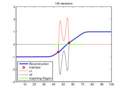
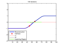
Figure 2: Here we present two numerical experiments related to the interpolation of a 1D signal by total variation minimization, provided only information only out of an interval (indicated in green color in the figures). On the left we show an application of algorithm (6) when no correction with the partition of unity is provided. In this case, the sequence of the local iterations u1(n),u2(n)superscriptsubscript𝑢1𝑛superscriptsubscript𝑢2𝑛u_{1}^{(n)},u_{2}^{(n)} is unbounded. On the right we show an application of algorithm (6) with the use of the partition of unity which enforces also the uniform boundedness of the local iterations u1(n),u2(n)superscriptsubscript𝑢1𝑛superscriptsubscript𝑢2𝑛u_{1}^{(n)},u_{2}^{(n)}.

A few technical tricks are additionally required for the boundedness of the iterations in algorithm (6) with respect to the nonoverlapping version. First of all the local minimizations are restricted to functions which vanish on the internal boundaries. Moreover since u(n)superscript𝑢𝑛u^{(n)} is formed as a sum of local components u1(n),u2(n)superscriptsubscript𝑢1𝑛superscriptsubscript𝑢2𝑛u_{1}^{(n)},u_{2}^{(n)} which are not uniquely determined on the overlapping part, we introduced a suitable correction by means of the partition of unity {χj:j=1,2}conditional-setsubscript𝜒𝑗𝑗12\{\chi_{j}:j=1,2\} in order to enforce the uniform boundedness of the sequences of the local iterations u1(n),u2(n)superscriptsubscript𝑢1𝑛superscriptsubscript𝑢2𝑛u_{1}^{(n)},u_{2}^{(n)}. With similar minor modifications, we can analogously formulate a parallel version of this algorithm as in (5).

4.2 The solution of the local iterations

The inner iterations

uj(n+1,+1)=argminΓjuj=0ujVj𝒥js(uj+ujˇ(n),uj(n+1,)),superscriptsubscript𝑢𝑗𝑛11subscriptargminsuperscriptsubscriptΓ𝑗subscript𝑢𝑗0subscript𝑢𝑗subscript𝑉𝑗superscriptsubscript𝒥𝑗𝑠subscript𝑢𝑗superscriptsubscript𝑢ˇ𝑗𝑛superscriptsubscript𝑢𝑗𝑛1u_{j}^{(n+1,\ell+1)}=\operatorname{argmin}_{\stackrel{{\scriptstyle u_{j}\in V_{j}}}{{\Gamma_{j}u_{j}=0}}}\mathcal{J}_{j}^{s}(u_{j}+u_{\check{j}}^{(n)},u_{j}^{(n+1,\ell)}),

where Γjuj=0subscriptΓ𝑗subscript𝑢𝑗0\Gamma_{j}u_{j}=0 is some linear constraint, are crucial for the concrete realizability of the algorithm. (Note that in the case of the nonoverlapping decomposition there is no additional linear constraint, whereas for the overlapping case we ask for the trace condition Γjuj=uj|Γj=0subscriptΓ𝑗subscript𝑢𝑗evaluated-atsubscript𝑢𝑗subscriptΓ𝑗0\Gamma_{j}u_{j}=u_{j}|_{\Gamma_{j}}=0.) Such iteration can be explicitely computed

uj(n+1,+1)superscriptsubscript𝑢𝑗𝑛11\displaystyle u_{j}^{(n+1,\ell+1)} =\displaystyle= [IπαK](uj(n+1,)+πVjT(gTujˇTuj(n+1,))\displaystyle\left[I-\pi_{\alpha K}\right]\left(u_{j}^{(n+1,\ell)}+\pi_{V_{j}}T^{*}(g-Tu_{\check{j}}-Tu_{j}^{(n+1,\ell)})\right.
+ujˇη(n+1,))ujˇ,\displaystyle\left.\phantom{XXXXXXXXX}+u_{\check{j}}-\eta^{(n+1,\ell)}\right)-u_{\check{j}},

for a suitable Lagrange multiplier η(n+1,)superscript𝜂𝑛1\eta^{(n+1,\ell)} which has the role of enforcing the linear constraints ujVjsubscript𝑢𝑗subscript𝑉𝑗u_{j}\in V_{j} and Γjuj=0subscriptΓ𝑗subscript𝑢𝑗0\Gamma_{j}u_{j}=0; η(n+1,)superscript𝜂𝑛1\eta^{(n+1,\ell)} can be approximated by an iterative algorithm, see [10, Proposition 4.6] for details. Note that we have to implement repeatedly the projection παKsubscript𝜋𝛼𝐾\pi_{\alpha K} for which the Chambolle’s algorithm (1) is used. More efficient algorithms can also be used such as iterative Bregman distance methods [12] or Nesterov’s algorithm [11].

5 Convergence properties

These algorithms share common convergence properties, which are listed in the following theorem.
Theorem. (Convergence properties) The algorithms (4), (5), and (6) produce a sequence (u(n))nsubscriptsuperscript𝑢𝑛𝑛(u^{(n)})_{n\in\mathbb{N}} in \mathcal{H} with the following properties:

(i)𝒥(u(n))>𝒥(u(n+1))𝒥superscript𝑢𝑛𝒥superscript𝑢𝑛1\mathcal{J}(u^{(n)})>\mathcal{J}(u^{(n+1)}) for all n𝑛n\in\mathbb{N} (unless u(n)=u(n+1)superscript𝑢𝑛superscript𝑢𝑛1u^{(n)}=u^{(n+1)});

(ii) limnu(n+1)u(n)2=0subscript𝑛subscriptnormsuperscript𝑢𝑛1superscript𝑢𝑛20\lim_{n\to\infty}\|u^{(n+1)}-u^{(n)}\|_{2}=0;

(iii) the sequence (u(n))nsubscriptsuperscript𝑢𝑛𝑛(u^{(n)})_{n\in\mathbb{N}} has subsequences which converge in \mathcal{H}; if (u(nk))ksubscriptsuperscript𝑢subscript𝑛𝑘𝑘(u^{(n_{k})})_{k\in\mathbb{N}} is a converging subsequence, and u()superscript𝑢u^{(\infty)} is its limit, then u()superscript𝑢u^{(\infty)} is always a minimizer of 𝒥𝒥\mathcal{J} in the case of algorithm (6) (overlapping case), whereas for algorithms (4), (5) (sequential and parallel nonoverlapping cases) this can be ensured under certain sufficient technical conditions, see [10, Theorem 5.1 and Theorem 6.1] for details.

6 Numerical experiments

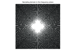
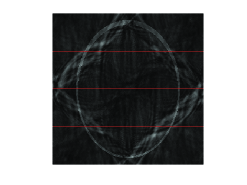
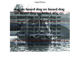
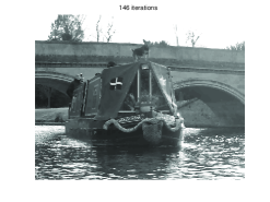
In the Figure 2, Figure 3, and Figure 4 we illustrate the results of several numerical experiments, showing the successful application of algorithms (4) and (6), for the restoration of 1D and 2D signals in interpolation/inpainting problems respectively, and for a compressed sensing problem.
Refer to caption
Refer to caption
Figure 3: This figure shows an application of algorithm (6) for an inpainting problem. In this simulation the problem was split via decomposition into four overlapping subdomains.
Refer to caption
Refer to caption
Refer to caption
Refer to caption
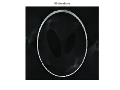
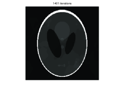
Figure 4: We show an application of algorithm (4) in a classical compressed sensing problem for recovering piecewise constant medical-type images from given partial Fourier data. In this simulation the problem was split via decomposition into four nonoverlapping subdomains. On the top-left figure, we show the sampling data of the image in the Fourier domain. On the top-right we show the back-projection provided by the sampled frequency data together with the highlighted partition of the physical domain into four subdomains. The bottom figures present intermediate iterations of the algorithm.

Acknowledgments

The authors acknowledge the support by the project WWTF Five senses-Call 2006, Mathematical Methods for Image Analysis and Processing in the Visual Arts. M. Fornasier acknowledges the financial support provided by START grant “Sparse Approximation and Optimization in High Dimensions” of the Austrian Science Fund. C.-B. Schönlieb acknowledges the financial support provided by KAUST (King Abdullah University of Science and Technology), by the Wissenschaftskolleg (Graduiertenkolleg, Ph.D. program) of the Faculty for Mathematics at the University of Vienna (funded by the Austrian Science Fund FWF), and by the FFG project Erarbeitung neuer Algorithmen zum Image Inpainting, projectnumber 813610.

References

  • [1] G. Aubert and P. Kornprobst, Mathematical Problems in Image Processing. Partial Differential Equations and the Calculus of Variation, Springer, 2002.
  • [2] E. J. Candés, J. Romberg, and T. Tao, Exact signal reconstruction from highly incomplete frequency information, IEEE Trans. Inf. Theory 52 (2006), no. 2, 489–509.
  • [3] A. Chambolle, An algorithm for total variation minimization and applications. J. Math. Imaging Vision 20 (2004), no. 1-2, 89–97.
  • [4] A. Chambolle and P.-L. Lions, Image recovery via total variation minimization and related problems., Numer. Math. 76 (1997), no. 2, 167–188.
  • [5] P. L. Combettes and V. R. Wajs, Signal recovery by proximal forward-backward splitting, Multiscale Model. Simul., 4 (2005), no. 4, 1168–1200.
  • [6] I. Daubechies, R. DeVore, M. Fornasier, and S. Güntürk, Iteratively re-weighted least squares minimization for sparse recovery, Commun. Pure Appl. Math. (2009) to appear, arXiv:0807.0575
  • [7] I. Daubechies, G. Teschke, and L. Vese, Iteratively solving linear inverse problems under general convex constraints, Inverse Probl. Imaging 1 (2007), no. 1, 29–46.
  • [8] D. L. Donoho, Compressed sensing, IEEE Trans. Inf. Theory 52 (2006), no. 4, 1289–1306.
  • [9] M. Fornasier, Domain decomposition methods for linear inverse problems with sparsity constraints, Inverse Problems 23 (2007), no. 6, 2505–2526.
  • [10] M. Fornasier and C.-B. Schönlieb, Subspace correction methods for total variation and 1limit-fromsubscript1\ell_{1}-minimization, arXiv:0712.2258 (2007)
  • [11] Y. Nesterov, Smooth minimization of non-smooth functions. Mathematic Programming, Ser. A, 103 (2005), 127–152.
  • [12] S. Osher, M. Burger, D. Goldfarb, J. Xu, and W. Yin, An Iterative Regularization Method for Total Variation-Based Image Restoration, Multiscale Model. Simul. 4, no. 2 (2005) 460-489.
  • [13] L. I. Rudin, S. Osher, and E. Fatemi, Nonlinear total variation based noise removal algorithms., Physica D 60 (1992), no. 1-4, 259–268.
  • [14] L. Vese, A study in the BV space of a denoising-deblurring variational problem., Appl. Math. Optim. 44 (2001), 131–161.
  • [15] P. Weiss, L. Blanc-Féraud, and G. Aubert, Efficient schemes for total variation minimization under constraints in image processing, SIAM J. Sci. Comput., (2009) to appear.