Cosmography and large scale structure by $f(R)$-gravity: new results

Abstract

The so called $f(R)$-gravity has recently attracted a lot of interest since it could be, in principle, able to explain the accelerated expansion of the Universe without adding unknown forms of dark energy/dark matter but, more simply, extending the General Relativity by generic functions of the Ricci scalar. However, apart several phenomenological models, there is no final $f(R)$-theory capable of fitting all the observations and addressing all the issues related to the presence of dark energy and dark matter. An alternative approach could be to "reconstruct" the form of $f(R)$ starting from data without imposing particular classes of model. In this review paper, we will consider two typical cosmological problems where the role of dark energy and dark matter is crucial. Firstly, assuming generic $f(R)$, we show that it is possible to relate the cosmographic parameters (namely the deceleration $q_{0}$, the jerk $j_{0}$, the snap $s_{0}$ and the lerk $l_{0}$ parameters) to the present day values of $f(R)$ and its derivatives $f^{(n)}(R)=d^{n}f/dR^{n}$ (with $n=1,2,3$) thus offering a new tool to constrain such higher order models. Our analysis gives the possibility to relate the model-independent results coming from cosmography to some theoretically motivated assumptions of $f(R)$ cosmology. Besides, adopting the same philosophy, we take into account the possibility that galaxy cluster masses, estimated at X-ray wavelengths, could be explained, without dark matter, reconstructing the weak-field limit of analytic $f(R)$ models. The corrected gravitational potential, obtained in this approximation, is used to estimate the total mass of a sample of $12$ well-shaped clusters of galaxies. Results show that such a gravitational potential provides a fair fit to the mass of visible matter (i.e. gas + stars) estimated by X-ray observations, without the need of additional dark matter while the size of the clusters, as already observed at different scale for galaxies, strictly depends on the interaction lengths of the corrections to the Newtonian potential. These two examples could be paradigmatic to overcome dark energy and dark matter problems by the extended gravity approach.

I Introduction

As soon as astrophysicists realized that Type Ia Supernovae (SNeIa) were standard candles, it appeared evident that their high luminosity should make it possible to build a Hubble diagram, i.e. a plot of the distance - redshift relation, over cosmologically interesting distance ranges. Motivated by this attractive consideration, two independent teams started SNeIa surveys leading to the unexpected discovery that the Universe expansion is speeding up rather than decelerating as assumed by the Cosmological Standard Model Perlm97 ; Perlm99 ; Riess98 ; Schmidt98 ; Garn98 . This surprising result has now been strengthened by more recent data coming from SNeIa surveys Knop03 ; Tonry03 ; Barris04 ; Riess04 ; R06 ; SNLS ; ESSENCE ; D07 , large scale structure Dode02 ; Perci02 ; Szal03 ; Hawk03 ; pope04 and cosmic microwave background (CMBR) anisotropy spectrum Boom ; Stomp01 ; Netter02 ; Rebo04 ; wmap ; WMAP ; WMAP3 . This large data set coherently points toward the picture of a spatially flat Universe undergoing an accelerated expansion driven by a dominant negative pressure fluid, typically referred to as dark energy copeland .

While there is a wide consensus on the above scenario depicted by such good quality data, there is a similarly wide range of contrasting proposals to solve the dark energy puzzle. Surprisingly, the simplest explanation, namely the cosmological constant $\Lambda$ CarLam ; Sahni , is also the best one from a statistical point of view Teg03 ; Teg06 ; Sel04 . Unfortunately, the well known coincidence and 120 orders of magnitude problems render $\Lambda$ a rather unattractive solution from a theoretical point of view. Inspired by the analogy with inflation, a scalar field $\phi$, dubbed quintessence PB03 ; Pad03 , has then been proposed to give a dynamical $\Lambda$ term in order to both fit the data and avoid the above problems. However, such models are still plagued by difficulties on their own, such as the almost complete freedom in the choice of the scalar field potential and the fine tuning of the initial conditions. Needless to say, a plethora of alternative models are now on the market all sharing the main property to be in agreement with observations, but relying on completely different physics.

Notwithstanding their differences, all dark energy models assume that the observed apparent acceleration is the outcome of some unknown ingredient, at fundamental level, to be added to the cosmic pie. In terms of the Einstein equations, $G_{\mu\nu}=\chi T_{\mu\nu}$, the right hand side should include something more than the usual matter and radiation components in the stress - energy tensor.

As a radically different approach, one can also try to leave unchanged the source side (actually "observed" since composed by radiation and baryonic matter), but rather modifying the left hand side. In a sense, one is therefore interpreting cosmic speed up as a first signal of the breakdown of the laws of physics as described by the standard General Relativity (GR). Since this theory has been experimentally tested only up to the Solar System scale, there is no a priori theoretical motivation to extend its validity to extraordinarily larger scales such as the extragalactic and cosmological ones (up to the last scattering surface!). Extending GR, not giving up to its positive results at local scales, opens the way to a large class of alternative theories of gravity ranging from extra - dimensions DGP ; DGP2 ; DGP3 ; Lue ; Lue2 to nonminimally coupled scalar fields stbook ; Care04 ; Petto05 ; Demia06 . In particular, we are interested here in fourth order theories alle04 ; capozzcurv ; noirev ; capfra ; noiijmpd ; cct ; sante ; cdtt ; Klein02 ; no03a ; odi03 ; nodi03 ; cdtt based on replacing the scalar curvature $R$ in the Hilbert–Einstein action with a generic analytic function $f(R)$ which should be reconstructed starting from data and physically motivated issues. Also referred to as $f(R)$-gravity, some of these models have been shown to be able to both fit the cosmological data and evade the Solar System constraints in several physically interesting cases Hu ; Starobinsky ; Appleby ; Odintsov ; Tsuji .

In this review paper, we will face two of the main problems directly related to the dark energy and dark matter issues: cosmography and clusters of galaxies. These are typical examples where the standard General Relativity and Newtonian potential schemes fail to describe dynamics since data present accelerated expansion and missing matter. Our goal is to address them by $f(R)$-gravity.

I.1 Cosmography: why?

It is worth noting that both dark energy models and modified gravity theories seem to be in agreement with data. As a consequence, unless higher precision probes of the expansion rate and the growth of structure will be available, these two rival approaches could not be discriminated. This confusion about the theoretical background suggests that a more conservative approach to the problem of cosmic acceleration, relying on as less model dependent quantities as possible, is welcome. A possible solution could be to come back to the cosmography W72 rather than finding out solutions of the Friedmann equations and testing them. Being only related to the derivatives of the scale factor, the cosmographic parameters make it possible to fit the data on the distance - redshift relation without any a priori assumption on the underlying cosmological model: in this case, the only assumption is that the metric is the Robertson - Walker one (and hence not relying on the solution of cosmological equations). Almost eighty years after Hubble discovery of the expansion of the Universe, we can now extend, in principle, cosmography well beyond the search for the value of the only Hubble constant. The SNeIa Hubble diagram extends up to $z=1.7$ thus invoking the need for, at least, a fifth order Taylor expansion of the scale factor in order to give a reliable approximation of the distance - redshift relation. As a consequence, it could be, in principle, possible to estimate up to five cosmographic parameters, although the still too small data set available does not allow to get a precise and realistic determination of all of them.

Once these quantities have been determined, one could use them to put constraints on the models. In a sense, we can revert the usual approach, consisting in deriving the cosmographic parameters as a sort of byproduct of an assumed theory. Here, we follow the other way around expressing the model characterizing quantities as a function of the cosmographic parameters. Such a program is particularly suited for the study of fourth order theories of gravity. As it is well known, the mathematical difficulties entering the solution of fourth order field equations make it quite problematic to find out analytical expressions for the scale factor and hence predict the values of the cosmographic parameters. A key role in $f(R)$-gravity is played by the choice of the $f(R)$ function. Under quite general hypotheses, we will derive useful relations among the cosmographic parameters and the present day value of $f^{(n)}(R)=d^{n}f/dR^{n}$, with $n=0,\ldots,3$, whatever $f(R)$ is. Once the cosmographic parameters will be determined, this method will allow us to investigate the cosmography of $f(R)$ theories.

It is worth stressing that the definition of the cosmographic parameters only relies on the assumption of the Robertson - Walker metric. As such, it is however difficult to state a priori to what extent the fifth order expansion provides an accurate enough description of the quantities of interest. Actually, the number of cosmographic parameters to be used depends on the problem one is interested in. As we will see later, we are here concerned only with the SNeIa Hubble diagram so that we have to check that the distance modulus $\mu_{cp}(z)$ obtained using the fifth order expansion of the scale factor is the same (within the errors) as the one $\mu_{DE}(z)$ of the underlying physical model. Being such a model of course unknown, one can adopt a phenomenological parameterization for the dark energy equation of state (EoS) and look at the percentage deviation $\Delta\mu/\mu_{DE}$ as function of the EoS parameters. We have carried out such exercise using the CPL model, introduced below, and verified that $\Delta\mu/\mu_{DE}$ is an increasing function of $z$ (as expected), but still remains smaller than $2\%$ up to $z\sim 2$ over a wide range of the CPL parameter space. On the other hand, halting the Taylor expansion to a lower order may introduce significant deviation for $z>1$ that can potentially bias the analysis if the measurement errors are as small as those predicted by future SNeIa surveys. We are therefore confident that our fifth order expansion is both sufficient to get an accurate distance modulus over the redshift range probed by SNeIa and necessary to avoid dangerous biases.

I.2 Clusters of galaxies: why?

In the second part of this review we will apply the $f(R)$-gravity approach to cluster of galaxies. In fact, changing the gravity sector has consequences not only at cosmological scales, but also at galactic and cluster scales so that it is mandatory to investigate the low energy limit of such theories. A strong debate is open with different results arguing in favor dick ; sotiriou ; cembranos ; navarro ; allrugg ; ppnantro or against dolgov ; chiba ; olmo such models at local scales. It is worth noting that, as a general result, higher order theories of gravity cause the gravitational potential to deviate from its Newtonian $1/r$ scaling b10 ; hj ; hjrev ; cb05 ; sobouti ; Mendoza even if such deviations may be vanishing.

In CapCardTro07 , the Newtonian limit of power law $f(R)=f_{0}R^{n}$ theories has been investigated, assuming that the metric in the low energy limit ($\Phi/c^{2}<<1$) may be taken as Schwarzschild - like. It turns out that a power law term $(r/r_{c})^{\beta}$ has to be added to the Newtonian $1/r$ term in order to get the correct gravitational potential. While the parameter $\beta$ may be expressed analytically as a function of the slope $n$ of the $f(R)$ theory, $r_{c}$ sets the scale where the correction term starts being significant. A particular range of values of $n$ has been investigated so that the corrective term is an increasing function of the radius $r$ thus causing an increase of the rotation curve with respect to the Newtonian one and offering the possibility to fit the galaxy rotation curves without the need of further dark matter components.

A set of low surface brightness (LSB) galaxies with extended and well measured rotation curves has been considered dbb02 ; db05 . These systems are supposed to be dark matter dominated, and successfully fitting data without dark matter is a strong evidence in favor of the approach (see also Frigerio for an independent analysis using another sample of galaxies). Combined with the hints coming from the cosmological applications, one should have, in principle, the possibility to address both the dark energy and dark matter problems resorting to the same well motivated fundamental theory fogdm ; prl ; Koivisto ; lobo . Nevertheless, the simple power law $f(R)$ gravity is nothing else but a toy-model which fail if one tries to achieve a comprehensive model for all the cosmological dynamics, ranging from the early Universe, to the large scale structure up to the late accelerated era prl ; Koivisto .

A fundamental issue is related to clusters and superclusters of galaxies. Such structures, essentially, rule the large scale structure, and are the intermediate step between galaxies and cosmology. As the galaxies, they appear dark-matter dominated but the distribution of dark matter component seems clustered and organized in a very different way with respect to galaxies. It seems that dark matter is ruled by the scale and also its fundamental nature could depend on the scale. For a comprehensive review see Bah96 .

In the philosophy of $f(R)$-gravity, the issue is to reconstruct the mass profile of clusters without dark matter, i.e. to find out corrections to the Newton potential producing the same dynamics as dark matter but starting from a well motivated theory.

In conclusion, $f(R)$-gravity, as the simplest approach to any extended or alternative gravity scheme, could be the paradigm to interpret dark energy and dark matter as curvature effects acting at scales larger than those where General Relativity has been actually investigated and probed.

Let us discuss now how cosmography and then galaxy clusters could be two main examples to realize this program.

II The cosmographic apparatus

The key rule in cosmography is the Taylor series expansion of the scale factor with respect to the cosmic time. To this aim, it is convenient to introduce the following functions:

$$H(t) \equiv +\frac{1}{a}\frac{da}{dt}\,,$$ (1)

$$q(t) \equiv -\frac{1}{a}\frac{d^{2}a}{dt^{2}}\frac{1}{H^{2}}\,,$$ (2)

$$j(t) \equiv +\frac{1}{a}\frac{d^{3}a}{dt^{3}}\frac{1}{H^{3}}\,,$$ (3)

$$s(t) \equiv +\frac{1}{a}\frac{d^{4}a}{dt^{4}}\frac{1}{H^{4}}\,,$$ (4)

$$l(t) \equiv +\frac{1}{a}\frac{d^{5}a}{dt^{5}}\frac{1}{H^{5}}\,,$$ (5)

which are usually referred to as the Hubble, deceleration, jerk, snap and lerk parameters, respectively. It is then a matter of algebra to demonstrate the following useful relations :

$$\dot{H} = -H^{2}(1+q)\ ,$$ (6)

$$\ddot{H} = H^{3}(j+3q+2)\ ,$$ (7)

$$d^{3}H/dt^{3} = H^{4}\left[s-4j-3q(q+4)-6\right]\ ,$$ (8)

$$d^{4}H/dt^{4} = H^{5}\left[l-5s+10(q+2)j+30(q+2)q+24\right]\ ,$$ (9)

where a dot denotes derivative with respect to the cosmic time $t$. Eqs.(6) - (9) make it possible to relate the derivative of the Hubble parameter to the other cosmographic parameters. The distance - redshift relation may then be obtained starting from the Taylor expansion of $a(t)$ along the lines described in Visser ; WM04 ; CV07 .

II.1 The scale-factor series

With these definitions the series expansion to the 5th order in time of the scale factor will be:

$$a(t) = a(t_{0})\left\{H_{0}(t-t_{0})-\frac{q_{0}}{2}H_{0}^{2}(t-t_{0})^{2}+\frac{j_{0}}{3!}H_{0}^{3}(t-t_{0})^{3}+\frac{s_{0}}{4!}H_{0}^{4}(t-t_{0})^{4}+\frac{l_{0}}{5!}H_{0}^{5}(t-t_{0})^{5}+\emph{O}[(t-t_{0})^{6}]\right\}$$ (10)

$$\frac{a(t)}{a(t_{0})} = 1+H_{0}(t-t_{0})-\frac{q_{0}}{2}H_{0}^{2}(t-t_{0})^{2}+\frac{j_{0}}{3!}H_{0}^{3}(t-t_{0})^{3}+\frac{s_{0}}{4!}H_{0}^{4}(t-t_{0})^{4}+\frac{l_{0}}{5!}H_{0}^{5}(t-t_{0})^{5}+\emph{O}[(t-t_{0})^{6}]$$ (11)

It’s easy to see that Eq.(11) is the inverse of redshift $z$, being the redshift defined by:

$$1+z=\frac{a(t_{0})}{a(t)}$$

The physical distance travelled by a photon that is emitted at time $t_{*}$ and absorbed at the current epoch $t_{0}$ is

$$D=c\int dt=c(t_{0}-t_{*})$$

Assuming $t_{*}=t_{0}-\frac{D}{c}$ and inserting in Eq.(11) we have:

$$1+z=\frac{a(t_{0})}{a(t_{0}-\frac{D}{c})}=\frac{1}{1-\frac{H_{0}}{c}D-\frac{q_{0}}{2}\left(\frac{H_{0}}{c}\right)^{2}D^{2}-\frac{j_{0}}{6}\left(\frac{H_{0}}{c}\right)^{3}D^{3}+\frac{s_{0}}{24}\left(\frac{H_{0}}{c}\right)^{4}D^{4}-\frac{l_{0}}{120}\left(\frac{H_{0}}{c}\right)^{5}D^{5}+\emph{O}[(\frac{H_{0}D}{c})^{6}]}$$ (12)

The inverse of this expression will be:

$$1+z = 1+\frac{H_{0}}{c}D+\left(1+\frac{q_{0}}{2}\right)\left(\frac{H_{0}}{c}\right)^{2}D^{2}+\left(1+q_{0}+\frac{j_{0}}{6}\right)\left(\frac{H_{0}}{c}\right)^{3}D^{3}+\left(1+\frac{3}{2}q_{0}+\frac{q_{0}^{2}}{4}+\frac{j_{0}}{3}-\frac{s_{0}}{24}\right)\left(\frac{H_{0}}{c}\right)^{4}D^{4}+$$ (13)

$$+ \left(1+2q_{0}+\frac{3}{4}q_{0}^{2}+\frac{q_{0}j_{0}}{6}+\frac{j_{0}}{2}-\frac{s}{12}+l_{0}\right)\left(\frac{H_{0}}{c}\right)^{5}D^{5}+\emph{O}\left[\left(\frac{H_{0}D}{c}\right)^{6}\right]$$

Then we reverse the series $z(D)\rightarrow D(z)$ to have the physical distance $D$ expressed as function of redshift $z$:

$$z(D) = \mathcal{Z}_{D}^{1}\left(\frac{H_{0}D}{c}\right)+\mathcal{Z}_{D}^{2}\left(\frac{H_{0}D}{c}\right)^{2}+\mathcal{Z}_{D}^{3}\left(\frac{H_{0}D}{c}\right)^{3}+\mathcal{Z}_{D}^{4}\left(\frac{H_{0}D}{c}\right)^{4}+\mathcal{Z}_{D}^{5}\left(\frac{H_{0}D}{c}\right)^{5}+\emph{O}\left[\left(\frac{H_{0}D}{c}\right)^{6}\right]$$ (14)

with:

$$\mathcal{Z}_{D}^{1} = 1$$ (15)

$$\mathcal{Z}_{D}^{2} = 1+\frac{q_{0}}{2}$$ (16)

$$\mathcal{Z}_{D}^{3} = 1+q_{0}+\frac{j_{0}}{6}$$ (17)

$$\mathcal{Z}_{D}^{4} = 1+\frac{3}{2}q_{0}+\frac{q_{0}^{2}}{4}+\frac{j_{0}}{3}-\frac{s_{0}}{24}$$ (18)

$$\mathcal{Z}_{D}^{5} = 1+2q_{0}+\frac{3}{4}q_{0}^{2}+\frac{q_{0}j_{0}}{6}+\frac{j_{0}}{2}-\frac{s}{12}+l_{0}$$ (19)

From this we have:

$$D(z) = \frac{cz}{H_{0}}\left\{\mathcal{D}_{z}^{0}+\mathcal{D}_{z}^{1}\ z+\mathcal{D}_{z}^{2}\ z^{2}+\mathcal{D}_{z}^{3}\ z^{3}+\mathcal{D}_{z}^{4}\ z^{4}+\emph{O}(z^{5})\right\}$$ (20)

with:

$$\mathcal{D}_{z}^{0} = 1$$ (21)

$$\mathcal{D}_{z}^{1} = -\left(1+\frac{q_{0}}{2}\right)$$ (22)

$$\mathcal{D}_{z}^{2} = 1+q_{0}+\frac{q_{0}^{2}}{2}-\frac{j_{0}}{6}$$ (23)

$$\mathcal{D}_{z}^{3} = -\left(1+\frac{3}{2}q_{0}+\frac{3}{2}q_{0}^{2}+\frac{5}{8}q_{0}^{3}-\frac{1}{2}j_{0}-\frac{5}{12}q_{0}j_{0}-\frac{s_{0}}{24}\right)$$ (24)

$$\mathcal{D}_{z}^{4} = 1+2q_{0}+3q_{0}^{2}+\frac{5}{2}q_{0}^{3}+\frac{7}{2}q_{0}^{4}-\frac{5}{3}q_{0}j_{0}-\frac{7}{8}q_{0}^{2}j_{0}-\frac{1}{8}q_{0}s_{0}-j_{0}+\frac{j_{0}^{2}}{12}-\frac{s_{0}}{6}-\frac{l_{0}}{120}$$ (25)

In typical applications, one is not interested in the physical distance $D(z)$, but other definitions:

• the luminosity distance:

  $$d_{L}=\frac{a(t_{0})}{a(t_{0}-\frac{D}{c})}\>(a(t_{0})r_{0})$$ (27)

• the angular-diameter distance:

  $$d_{A}=\frac{a(t_{0}-\frac{D}{c})}{a(t_{0})}\>(a(t_{0})r_{0})$$ (28)

where $r_{0}(D)$ is:

$$r_{0}(D)=\left\{\begin{array}[]{lr}\sin(\int_{t_{0}-\frac{D}{c}}^{t_{0}}\frac{c\ \mathrm{d}t}{a(t)})&k=+1;\\ &\\ \int_{t_{0}-\frac{D}{c}}^{t_{0}}\frac{c\ \mathrm{d}t}{a(t)}&k=0;\\ &\\ \sinh(\int_{t_{0}-\frac{D}{c}}^{t_{0}}\frac{c\ \mathrm{d}t}{a(t)})&k=-1.\end{array}\right.$$ (29)

If we make the expansion for short distances, namely if we insert the series expansion of $a(t)$ in $r_{0}(D)$, we have:

$$r_{0}(D) = \int_{t_{0}-\frac{D}{c}}^{t_{0}}\frac{c\ \mathrm{d}t}{a(t)}=\int_{t_{0}-\frac{D}{c}}^{t_{0}}\frac{c\ \mathrm{d}t}{a_{0}}\left\{1+H_{0}(t_{0}-t)+\left(1+\frac{q_{0}}{2}\right)H_{0}^{2}(t_{0}-t)^{2}+\left(1+q_{0}+\frac{j_{0}}{6}\right)H_{0}^{3}(t_{0}-t)^{3}+\right.$$ (30)

$$+ \left.\left(1+\frac{3}{2}q_{0}+\frac{q_{0}^{2}}{4}+\frac{j_{0}}{3}-\frac{s_{0}}{24}\right)H_{0}^{4}(t_{0}-t)^{4}+\left(1+2q_{0}+\frac{3}{4}q_{0}^{2}+\frac{q_{0}j_{0}}{6}+\frac{j_{0}}{2}-\frac{s}{12}+l_{0}\right)H_{0}^{5}(t_{0}-t)^{5}+\emph{O}[(t_{0}-t)^{6}]\right\}=$$

$$= \frac{D}{a_{0}}\left\{1+\frac{1}{2}\frac{H_{0}D}{c}+\left[\frac{2+q_{0}}{6}\right]\left(\frac{H_{0}D}{c}\right)^{2}+\left[\frac{6+6q_{0}+j_{0}}{24}\right]\left(\frac{H_{0}D}{c}\right)^{3}+\left[\frac{24+36q_{0}+6q_{0}^{2}+8j_{0}-s_{0}}{120}\right]\left(\frac{H_{0}D}{c}\right)^{4}+\right.$$

$$+ \left.\left[\frac{12+24q_{0}+9q_{0}^{2}+2q_{0}j_{0}+6j_{0}-s_{0}+12l_{0}}{72}\right]\left(\frac{H_{0}D}{c}\right)^{5}+\emph{O}\left[\left(\frac{H_{0}D}{c}\right)^{6}\right]\right\}$$

To convert from physical distance travelled to r coordinate traversed we have to consider that the Taylor series expansion of $\sin$-$\sinh$ functions is:

$$r_{0}(D)=\left[\int_{t_{0}-\frac{D}{c}}^{t_{0}}\frac{c\ \mathrm{d}t}{a(t)}\right]-\frac{k}{3!}\left[\int_{t_{0}-\frac{D}{c}}^{t_{0}}\frac{c\ \mathrm{d}t}{a(t)}\right]^{3}+\emph{O}\left(\left[\int_{t_{0}-\frac{D}{c}}^{t_{0}}\frac{c\ \mathrm{d}t}{a(t)}\right]^{5}\right)$$ (31)

so that Eq.(11) with curvature $k$ term becomes:

$$r_{0}(D) = \frac{D}{a_{0}}\left\{\mathcal{R}_{D}^{0}+\mathcal{R}_{D}^{1}\frac{H_{0}D}{c}+\mathcal{R}_{D}^{2}\left(\frac{H_{0}D}{c}\right)^{2}+\mathcal{R}_{D}^{3}\left(\frac{H_{0}D}{c}\right)^{3}+\right.$$ (32)

$$+ \left.\mathcal{R}_{D}^{4}\left(\frac{H_{0}D}{c}\right)^{4}+\mathcal{R}_{D}^{5}\left(\frac{H_{0}D}{c}\right)^{5}+\emph{O}\left[\left(\frac{H_{0}D}{c}\right)^{6}\right]\right\}$$

with:

$$\mathcal{R}_{D}^{0} = 1$$ (33)

$$\mathcal{R}_{D}^{1} = \frac{1}{2}$$ (34)

$$\mathcal{R}_{D}^{2} = \frac{1}{6}\left[2+q_{0}-\frac{kc^{2}}{H_{0}^{2}a_{0}^{2}}\right]$$ (35)

$$\mathcal{R}_{D}^{3} = \frac{1}{24}\left[6+6q_{0}+j_{0}-6\frac{kc^{2}}{H_{0}^{2}a_{0}^{2}}\right]$$ (36)

$$\mathcal{R}_{D}^{4} = \frac{1}{120}\left[24+36q_{0}+6q_{0}^{2}+8j_{0}-s_{0}-\frac{5kc^{2}(7+2q_{0})}{a_{0}^{2}H_{0}^{2}}\right]$$ (37)

$$\mathcal{R}_{D}^{5} = \frac{1}{144}\left[24+48q_{0}+18q_{0}^{2}+4q_{0}j_{0}+12j_{0}-2s_{0}+24l_{0}-\frac{3kc^{2}(15+10q_{0}+j_{0})}{a_{0}^{2}H_{0}^{2}}\right]$$ (38)

Using these one for luminosity distance we have:

$$d_{L}(z)=\frac{cz}{H_{0}}\left\{\mathcal{D}_{L}^{0}+\mathcal{D}_{L}^{1}\ z+\mathcal{D}_{L}^{2}\ z^{2}+\mathcal{D}_{L}^{3}\ z^{3}+\mathcal{D}_{L}^{4}\ z^{4}+\emph{O}(z^{5})\right\}$$ (39)

with:

$$\mathcal{D}_{L}^{0} = 1$$ (40)

$$\mathcal{D}_{L}^{1} = -\frac{1}{2}\left(-1+q_{0}\right)$$ (41)

$$\mathcal{D}_{L}^{2} = -\frac{1}{6}\left(1-q_{0}-3q_{0}^{2}+j_{0}+\frac{kc^{2}}{H_{0}^{2}a_{0}^{2}}\right)$$ (42)

$$\mathcal{D}_{L}^{3} = \frac{1}{24}\left(2-2q_{0}-15q_{0}^{2}-15q_{0}^{3}+5j_{0}+10q_{0}j_{0}+s_{0}+\frac{2kc^{2}(1+3q_{0})}{H_{0}^{2}a_{0}^{2}}\right)$$ (43)

$$\mathcal{D}_{L}^{4} = \frac{1}{120}\left[-6+6q_{0}+81q_{0}^{2}+165q_{0}^{3}+105q_{0}^{4}-110q_{0}j_{0}-105q_{0}^{2}j_{0}-15q_{0}s_{0}+\right.$$ (44)

$$- \left.27j_{0}+10j^{2}-11s_{0}-l_{0}-\frac{5kc^{2}(1+8q_{0}+9q_{0}^{2}-2j_{0})}{a_{0}^{2}H_{0}^{2}}\right]$$ (45)

While for the angular diameter distance it is:

$$d_{A}(z)=\frac{cz}{H_{0}}\left\{\mathcal{D}_{A}^{0}+\mathcal{D}_{A}^{1}\ z+\mathcal{D}_{A}^{2}\ z^{2}+\mathcal{D}_{A}^{3}\ z^{3}+\mathcal{D}_{A}^{4}\ z^{4}+\emph{O}(z^{5})\right\}$$ (46)

with:

$$\mathcal{D}_{A}^{0} = 1$$ (47)

$$\mathcal{D}_{A}^{1} = -\frac{1}{2}\left(3+q_{0}\right)$$ (48)

$$\mathcal{D}_{A}^{2} = \frac{1}{6}\left[11+7q_{0}+3q_{0}^{2}-j_{0}-\frac{kc^{2}}{H_{0}^{2}a_{0}^{2}}\right]$$ (49)

$$\mathcal{D}_{A}^{3} = -\frac{1}{24}\left[50+46q_{0}+39q_{0}^{2}+15q_{0}^{3}-13j_{0}-10q_{0}j_{0}-s_{0}-\frac{2kc^{2}(5+3q_{0})}{H_{0}^{2}a_{0}^{2}}\right]$$ (50)

$$\mathcal{D}_{A}^{4} = \frac{1}{120}\left[274+326q_{0}+411q_{0}^{2}+315q_{0}^{3}+105q_{0}^{4}-210q_{0}j_{0}-105q_{0}^{2}j_{0}-15q_{0}s_{0}+\right.$$ (51)

$$- \left.137j_{0}+10j^{2}-21s_{0}-l_{0}-\frac{5kc^{2}(17+20q_{0}+9q_{0}^{2}-2j_{0})}{a_{0}^{2}H_{0}^{2}}\right]$$ (52)

If we want to use the same notation of CV07 , we define $\Omega_{0}=1+\frac{kc^{2}}{H_{0}^{2}a_{0}^{2}}$, which can be considered a purely cosmographic parameter, or $\Omega_{0}=1-\Omega_{k}=\Omega_{m,0}+\Omega_{r,0}+\Omega_{X,0}$ if we consider the dynamics of the Universe. With this parameter Eqs.(26)-(28) become:

$$\mathcal{D}_{L,y}^{0} = 1$$ (53)

$$\mathcal{D}_{L,y}^{1} = -\frac{1}{2}\left(-3+q_{0}\right)$$ (54)

$$\mathcal{D}_{L,y}^{2} = -\frac{1}{6}\left(12-5q_{0}+3q_{0}^{2}-j_{0}-\Omega_{0}\right)$$ (55)

$$\mathcal{D}_{L,y}^{3} = \frac{1}{24}\left[52-20q_{0}+21q_{0}^{2}-15q_{0}^{3}-7j_{0}+10q_{0}j_{0}+s_{0}-2\Omega_{0}(1+3q_{0})\right]$$ (56)

$$\mathcal{D}_{L,y}^{4} = \frac{1}{120}\left[359-184q_{0}+186q_{0}^{2}-135q_{0}^{3}+105q_{0}^{4}+90q_{0}j_{0}-105q_{0}^{2}j_{0}-15q_{0}s_{0}+\right.$$ (57)

$$- \left.57j_{0}+10j^{2}+9s_{0}-l_{0}-5\Omega_{0}(17-6q_{0}+9q_{0}^{2}-2j_{0})\right]$$ (58)

and

$$\mathcal{D}_{A,y}^{0} = 1$$ (59)

$$\mathcal{D}_{A,y}^{1} = -\frac{1}{2}\left(1+q_{0}\right)$$ (60)

$$\mathcal{D}_{A,y}^{2} = -\frac{1}{6}\left[-q_{0}-3q_{0}^{2}+j_{0}+\Omega_{0}\right]$$ (61)

$$\mathcal{D}_{A,y}^{3} = -\frac{1}{24}\left[-2q_{0}+3q_{0}^{2}+15q_{0}^{3}-j_{0}-10q_{0}j_{0}-s_{0}+2\Omega_{0}\right]$$ (62)

$$\mathcal{D}_{A,y}^{4} = -\frac{1}{120}\left[1-6q_{0}+9q_{0}^{2}-15q_{0}^{3}-105q_{0}^{4}+10q_{0}j_{0}+105q_{0}^{2}j_{0}+15q_{0}s_{0}+\right.$$ (63)

$$- \left.3j_{0}-10j^{2}+s_{0}+l_{0}+5\Omega_{0}\right]$$ (64)

Previous relations in this section have been derived for any value of the curvature parameter; but since in the following we will assume a flat Universe, we will used the simplified versions for $k=0$. Now, since we are going to use supernovae data, it will be useful to give as well the Taylor series of the expansion of the luminosity distance at it enters the modulus distance, which is the quantity about which those observational data inform. The final expression for the modulus distance based on the Hubble free luminosity distance, $\mu(z)=5\log_{10}d_{L}(z)$, is:

$$\mu(z)=\frac{5}{\log 10}\cdot\left(\log z+\mathcal{M}^{1}z+\mathcal{M}^{2}z^{2}+\mathcal{M}^{3}z^{3}+\mathcal{M}^{4}z^{4}\right)\,,$$ (65)

with

$$\mathcal{M}^{1} = -\frac{1}{2}\left[-1+q_{0}\right]\,,$$ (66)

$$\mathcal{M}^{2} = -\frac{1}{24}\left[7-10q_{0}-9q_{0}^{2}+4j_{0}\right]\,,$$ (67)

$$\mathcal{M}^{3} = \frac{1}{24}\left[5-9q_{0}-16q_{0}^{2}-10q_{0}^{3}+7j_{0}+8q_{0}j_{0}+s_{0}\right]\,,$$ (68)

$$\mathcal{M}^{4} = \frac{1}{2880}\left[-469+1004q_{0}+2654q_{0}^{2}+3300q_{0}^{3}+1575q_{0}^{4}+200j_{0}^{2}-1148j_{0}+\right.$$ (69)

$$- \left.-2620q_{0}j_{0}-1800q_{0}^{2}j_{0}-300q_{0}s_{0}-324s_{0}-24l_{0}\right]\,.$$

III $f(R)$-gravity vs cosmography

III.1 $f(R)$ preliminaries

As discussed in the Introduction, much interest has been recently devoted to the possibility that dark energy could be nothing else but a curvature effect according to which the present Universe is filled by pressureless dust matter only and the acceleration is the result of modified Friedmann equations obtained by replacing the Ricci curvature scalar $R$ with a generic function $f(R)$ in the gravity action. Under the assumption of a flat Universe, the Hubble parameter is therefore determined by :

$$H^{2}=\frac{1}{3}\left[\frac{\rho_{m}}{f^{\prime}(R)}+\rho_{curv}\right]$$ (70)

where the prime denotes derivative with respect to $R$ and $\rho_{curv}$ is the energy density of an effective curvature fluid :

$$\rho_{curv}=\frac{1}{f^{\prime}(R)}\left\{\frac{1}{2}\left[f(R)-Rf^{\prime}(R)\right]-3H\dot{R}f^{\prime\prime}(R)\right\}\ .$$ (71)

Assuming there is no interaction between the matter and the curvature terms (we are in the so-called Jordan frame), the matter continuity equation gives the usual scaling $\rho_{M}=\rho_{M}(t=t_{0})a^{-3}=3H_{0}^{2}\Omega_{M}a^{-3}$, with $\Omega_{M}$ the present day matter density parameter. The continuity equation for $\rho_{curv}$ then reads :

$$\dot{\rho}_{curv}+3H(1+w_{curv})\rho_{curv}=\frac{3H_{0}^{2}\Omega_{M}\dot{R}f^{\prime\prime}(R)}{\left[f^{\prime}(R)\right]^{2}}a^{-3}$$ (72)

with

$$w_{curv}=-1+\frac{\ddot{R}f^{\prime\prime}(R)+\dot{R}\left[\dot{R}f^{\prime\prime\prime}(R)-Hf^{\prime\prime}(R)\right]}{\left[f(R)-Rf^{\prime}(R)\right]/2-3H\dot{R}f^{\prime\prime}(R)}$$ (73)

the barotropic factor of the curvature fluid. It is worth noticing that the curvature fluid quantities $\rho_{curv}$ and $w_{curv}$ only depends on $f(R)$ and its derivatives up to the third order. As a consequence, considering only their present day values (which may be naively obtained by replacing $R$ with $R_{0}$ everywhere), two $f(R)$ theories sharing the same values of $f(R_{0})$, $f^{\prime}(R_{0})$, $f^{\prime\prime}(R_{0})$, $f^{\prime\prime\prime}(R_{0})$ will be degenerate from this point of view.

Combining Eq.(72) with Eq.(70), one finally gets the following master equation for the Hubble parameter :

$$\dot{H} = -\frac{1}{2f^{\prime}(R)}\left\{3H_{0}^{2}\Omega_{M}a^{-3}+\ddot{R}f^{\prime\prime}(R)+\right.$$

$$\left.+\dot{R}\left[\dot{R}f^{\prime\prime\prime}(R)-Hf^{\prime\prime}(R)\right]\right\}\ .$$ (74)

Expressing the scalar curvature $R$ as function of the Hubble parameter as :

$$R=-6\left(\dot{H}+2H^{2}\right)$$ (75)

and inserting the result into Eq.(74), one ends with a fourth order nonlinear differential equation for the scale factor $a(t)$ that cannot be easily solved also for the simplest cases (for instance, $f(R)\propto R^{n}$). Moreover, although technically feasible, a numerical solution of Eq.(74) is plagued by the large uncertainties on the boundary conditions (i.e., the present day values of the scale factor and its derivatives up to the third order) that have to be set to find out the scale factor.

III.2 $f(R)$-derivatives and cosmography

Motivated by these difficulties, we approach now the problem from a different viewpoint. Rather than choosing a parameterized expression for $f(R)$ and then numerically solving Eq.(74) for given values of the boundary conditions, we try to relate the present day values of its derivatives to the cosmographic parameters $(q_{0},j_{0},s_{0},l_{0})$ so that constraining them in a model independent way gives us a hint for what kind of $f(R)$ theory could be able to fit the observed Hubble diagram.

As a preliminary step, it is worth considering again the constraint equation (75). Differentiating with respect to $t$, we easily get the following relations :

$$\begin{array}[]{l}\displaystyle{\dot{R}=-6\left(\ddot{H}+4H\dot{H}\right)}\\ \nobreak\leavevmode\\ \displaystyle{\ddot{R}=-6\left(d^{3}H/dt^{3}+4H\ddot{H}+4\dot{H}^{2}\right)}\\ \nobreak\leavevmode\\ \displaystyle{d^{3}R/dt^{3}{R}=-6\left(d^{4}H/dt^{4}+4Hd^{3}H/dt^{3}+12\dot{H}\ddot{H}\right)}\\ \end{array}\ .$$ (76)

Evaluating these at the present time and using Eqs.(6) - (9), one finally gets :

$$R_{0}=-6H_{0}^{2}(1-q_{0})\ ,$$ (77)

$$\dot{R}_{0}=-6H_{0}^{3}(j_{0}-q_{0}-2)\ ,$$ (78)

$$\ddot{R}_{0}=-6H_{0}^{4}\left(s_{0}+q_{0}^{2}+8q_{0}+6\right)\ ,$$ (79)

$$d^{3}R_{0}/dt^{3}=-6H_{0}^{5}\left[l_{0}-s_{0}+2(q_{0}+4)j_{0}-6(3q_{0}+8)q_{0}-24\right]\ ,$$ (80)

which will turn out to be useful in the following.

Let us now come back to the expansion rate and master equations (70) and (74). Since they have to hold along the full evolutionary history of the Universe, they naively hold also at the present day. As a consequence, we may evaluate them in $t=t_{0}$ thus easily obtaining :

$$H_{0}^{2}=\frac{H_{0}^{2}\Omega_{M}}{f^{\prime}(R_{0})}+\frac{f(R_{0})-R_{0}f^{\prime}(R_{0})-6H_{0}\dot{R}_{0}f^{\prime\prime}(R_{0})}{6f^{\prime}(R_{0})}\ ,$$ (81)

$$-\dot{H}_{0}=\frac{3H_{0}^{2}\Omega_{M}}{2f^{\prime}(R_{0})}+\frac{\dot{R}_{0}^{2}f^{\prime\prime\prime}(R_{0})+\left(\ddot{R}_{0}-H_{0}\dot{R_{0}}\right)f^{\prime\prime}(R_{0})}{2f^{\prime}(R_{0})}\ .$$ (82)

Using Eqs.(6) - (9) and (77) - (80), we can rearrange Eqs.(81) and (82) as two relations among the Hubble constant $H_{0}$ and the cosmographic parameters $(q_{0},j_{0},s_{0})$, on one hand, and the present day values of $f(R)$ and its derivatives up to third order. However, two further relations are needed in order to close the system and determine the four unknown quantities $f(R_{0})$, $f^{\prime}(R_{0})$, $f^{\prime\prime}(R_{0})$, $f^{\prime\prime\prime}(R_{0})$. A first one may be easily obtained by noting that, inserting back the physical units, the rate expansion equation reads :

$$H^{2}=\frac{8\pi G}{3f^{\prime}(R)}\left[\rho_{m}+\rho_{curv}f^{\prime}(R)\right]$$

which clearly shows that, in $f(R)$ gravity, the Newtonian gravitational constant $G$ is replaced by an effective (time dependent) $G_{eff}=G/f^{\prime}(R)$. On the other hand, it is reasonable to assume that the present day value of $G_{eff}$ is the same as the Newtonian one so that we get the simple constraint :

$$G_{eff}(z=0)=G\rightarrow f^{\prime}(R_{0})=1\ .$$ (83)

In order to get the fourth relation we need to close the system, we first differentiate both sides of Eq.(74) with respect to $t$. We thus get :

$$\ddot{H} = \frac{\dot{R}^{2}f^{\prime\prime\prime}(R)+\left(\ddot{R}-H\dot{R}\right)f^{\prime\prime}(R)+3H_{0}^{2}\Omega_{M}a^{-3}}{2\left[\dot{R}f^{\prime\prime}(R)\right]^{-1}\left[f^{\prime}(R)\right]^{2}}-\frac{\dot{R}^{3}f^{(iv)}(R)+\left(3\dot{R}\ddot{R}-H\dot{R}^{2}\right)f^{\prime\prime\prime}(R)}{2f^{\prime}(R)}$$

$$- \frac{\left(d^{3}R/dt^{3}-H\ddot{R}+\dot{H}\dot{R}\right)f^{\prime\prime}(R)-9H_{0}^{2}\Omega_{M}Ha^{-3}}{2f^{\prime}(R)}\ ,$$ (84)

with $f^{(iv)}(R)=d^{4}f/dR^{4}$. Let us now suppose that $f(R)$ may be well approximated by its third order Taylor expansion in $R-R_{0}$, i.e. we set :

$$f(R)=f(R_{0})+f^{\prime}(R_{0})(R-R_{0})+\frac{1}{2}f^{\prime\prime}(R_{0})(R-R_{0})^{2}+\frac{1}{6}f^{\prime\prime\prime}(R_{0})(R-R_{0})^{3}\ .$$ (85)

In such an approximation, it is $f^{(n)}(R)=d^{n}f/R^{n}=0$ for $n\geq 4$ so that naively $f^{(iv)}(R_{0})=0$. Evaluating then Eq.(84) at the present day, we get :

$$\ddot{H}_{0} = \frac{\dot{R}_{0}^{2}f^{\prime\prime\prime}(R_{0})+\left(\ddot{R}_{0}-H_{0}\dot{R}_{0}\right)f^{\prime\prime}(R_{0})+3H_{0}^{2}\Omega_{M}}{2\left[\dot{R}_{0}f^{\prime\prime}(R_{0})\right]^{-1}\left[f^{\prime}(R_{0})\right]^{2}}-\frac{\left(3\dot{R}_{0}\ddot{R}_{0}-H\dot{R}_{0}^{2}\right)f^{\prime\prime\prime}(R_{0})}{2f^{\prime}(R_{0})}$$

$$- \frac{\left(d^{3}R_{0}/dt^{3}-H_{0}\ddot{R}_{0}+\dot{H}_{0}\dot{R}_{0}\right)f^{\prime\prime}(R_{0})-9H_{0}^{3}\Omega_{M}}{2f^{\prime}(R_{0})}\ .$$ (86)

We can now schematically proceed as follows. Evaluate Eqs.(6) - (9) at $z=0$ and plug these relations into the left hand sides of Eqs.(81), (82), (86). Insert Eqs.(77) - (80) into the right hand sides of these same equations so that only the cosmographic parameters $(q_{0},j_{0},s_{0},l_{0})$ and the $f(R)$ related quantities enter both sides of these relations. Finally, solve them under the constraint (83) with respect to the present day values of $f(R)$ and its derivatives up to the third order. After some algebra, one ends up with the desired result :

$$\frac{f(R_{0})}{6H_{0}^{2}}=-\frac{{\cal{P}}_{0}(q_{0},j_{0},s_{0},l_{0})\Omega_{M}+{\cal{Q}}_{0}(q_{0},j_{0},s_{0},l_{0})}{{\cal{R}}(q_{0},j_{0},s_{0},l_{0})}\ ,$$ (87)

$$f^{\prime}(R_{0})=1\ ,$$ (88)

$$\frac{f^{\prime\prime}(R_{0})}{\left(6H_{0}^{2}\right)^{-1}}=-\frac{{\cal{P}}_{2}(q_{0},j_{0},s_{0})\Omega_{M}+{\cal{Q}}_{2}(q_{0},j_{0},s_{0})}{{\cal{R}}(q_{0},j_{0},s_{0},l_{0})}\ ,$$ (89)

$$\frac{f^{\prime\prime\prime}(R_{0})}{\left(6H_{0}^{2}\right)^{-2}}=-\frac{{\cal{P}}_{3}(q_{0},j_{0},s_{0},l_{0})\Omega_{M}+{\cal{Q}}_{3}(q_{0},j_{0},s_{0},l_{0})}{(j_{0}-q_{0}-2){\cal{R}}(q_{0},j_{0},s_{0},l_{0})}\ ,$$ (90)

where we have defined :

$${\cal{P}}_{0} = (j_{0}-q_{0}-2)l_{0}-(3s_{0}+7j_{0}+6q_{0}^{2}+41q_{0}+22)s_{0}-\left[(3q_{0}+16)j_{0}+20q_{0}^{2}+64q_{0}+12\right]j_{0}+$$ (91)

$$- \left(3q_{0}^{4}+25q_{0}^{3}+96q_{0}^{2}+72q_{0}+20\right)\ ,$$

$${\cal{Q}}_{0} = (q_{0}^{2}-j_{0}q_{0}+2q_{0})l_{0}+\left[3q_{0}s_{0}+(4q_{0}+6)j_{0}+6q_{0}^{3}+44q_{0}^{2}+22q_{0}-12\right]s_{0}$$

$$+ \left[2j_{0}^{2}+(3q_{0}^{2}+10q_{0}-6)j_{0}+17q_{0}^{3}+52q_{0}^{2}+54q_{0}+36\right]j_{0}+3q_{0}^{5}+28q_{0}^{4}+118q_{0}^{3}+$$ (92)

$$+ 72q_{0}^{2}-76q_{0}-64\ ,$$

$${\cal{P}}_{2}=9s_{0}+6j_{0}+9q_{0}^{2}+66q_{0}+42\ ,$$ (93)

$${\cal{Q}}_{2} = -\left\{6(q_{0}+1)s_{0}+\left[2j_{0}-2(1-q_{0})\right]j_{0}+6q_{0}^{3}+50q_{0}^{2}+74q_{0}+32\right\}\ ,$$ (94)

$${\cal{P}}_{3}=3l_{0}+3s_{0}-9(q_{0}+4)j_{0}-(45q_{0}^{2}+78q_{0}+12)\ ,$$ (95)

$${\cal{Q}}_{3} = -\left\{2(1+q_{0})l_{0}+2(j_{0}+q_{0})s_{0}-(2j_{0}+4q_{0}^{2}+12q_{0}+6)j_{0}-(30q_{0}^{3}+84q_{0}^{2}+78q_{0}+24)\right\}\,$$ (96)

$${\cal{R}} = (j_{0}-q_{0}-2)l_{0}-(3s_{0}-2j_{0}+6q_{0}^{2}+50q_{0}+40)s_{0}+\left[(3q_{0}+10)j_{0}+11q_{0}^{2}+4q_{0}+\right.$$ (97)

$$- \left.18\right]j_{0}-(3q_{0}^{4}+34q_{0}^{3}+246q_{0}+104)\ .$$

Eqs.(87) - (97) make it possible to estimate the present day values of $f(R)$ and its first three derivatives as function of the Hubble constant $H_{0}$ and the cosmographic parameters $(q_{0},j_{0},s_{0},l_{0})$ provided a value for the matter density parameter $\Omega_{M}$ is given. This is a somewhat problematic point. Indeed, while the cosmographic parameters may be estimated in a model independent way, the fiducial value for $\Omega_{M}$ is usually the outcome of fitting a given dataset in the framework of an assumed dark energy scenario. However, it is worth noting that different models all converge towards the concordance value $\Omega_{M}\simeq 0.25$ which is also in agreement with astrophysical (model independent) estimates from the gas mass fraction in galaxy clusters. On the other hand, it has been proposed that $f(R)$ theories may avoid the need for dark matter in galaxies and galaxy clusters noipla ; prl ; CapCardTro07 ; Frigerio ; sobouti ; Mendoza ; fogdm . In such a case, the total matter content of the Universe is essentially equal to the baryonic one. According to the primordial elements abundance and the standard BBN scenario, we therefore get $\Omega_{M}\simeq\omega_{b}/h^{2}$ with $\omega_{b}=\Omega_{b}h^{2}\simeq 0.0214$ Kirk and $h$ the Hubble constant in units of $100{\rm km/s/Mpc}$. Setting $h=0.72$ in agreement with the results of the HST Key project Freedman , we thus get $\Omega_{M}=0.041$ for a baryons only Universe. We will therefore consider in the following both cases when numerical estimates are needed.

It is worth noticing that $H_{0}$ only plays the role of a scaling parameter giving the correct physical dimensions to $f(R)$ and its derivatives. As such, it is not surprising that we need four cosmographic parameters, namely $(q_{0},j_{0},s_{0},l_{0})$, to fix the four $f(R)$ related quantities $f(R_{0})$, $f^{\prime}(R_{0})$, $f^{\prime\prime}(R_{0})$, $f^{\prime\prime\prime}(R_{0})$. It is also worth stressing that Eqs.(87) - (90) are linear in the $f(R)$ quantities so that $(q_{0},j_{0},s_{0},l_{0})$ uniquely determine the former ones. On the contrary, inverting them to get the cosmographic parameters as function of the $f(R)$ ones, we do not get linear relations. Indeed, the field equations in $f(R)$ theories are nonlinear fourth order differential equations in the scale factor $a(t)$ so that fixing the derivatives of $f(R)$ up to third order makes it possible to find out a class of solutions, not a single one. Each one of these solutions will be characterized by a different set of cosmographic parameters thus explaining why the inversion of Eqs.(87) - (97) does not give a unique result for $(q_{0},j_{0},s_{0},l_{0})$.

As a final comment, we reconsider the underlying assumptions leading to the above derived relations. While Eqs.(81) and (82) are exact relations deriving from a rigorous application of the field equations, Eq.(86) heavily relies on having approximated $f(R)$ with its third order Taylor expansion (85). If this assumption fails, the system should not be closed since a fifth unknown parameter enters the game, namely $f^{(iv)}(R_{0})$. Actually, replacing $f(R)$ with its Taylor expansion is not possible for all class of $f(R)$ theories. As such, the above results only hold in those cases where such an expansion is possible. Moreover, by truncating the expansion to the third order, we are implicitly assuming that higher order terms are negligible over the redshift range probed by the data. That is to say, we are assuming that :

$$f^{(n)}(R_{0})(R-R_{0})^{n}<<\sum_{m=0}^{3}{\frac{f^{(m)}(R_{0})}{m!}(R-R_{0})^{m}}\ \ {\rm for}\ n\geq 4$$ (98)

over the redshift range probed by the data. Checking the validity of this assumption is not possible without explicitly solving the field equations, but we can guess an order of magnitude estimate considering that, for all viable models, the background dynamics should not differ too much from the $\Lambda$CDM one at least up to $z\simeq 2$. Using then the expression of $H(z)$ for the $\Lambda$CDM model, it is easily to see that $R/R_{0}$ is a quickly increasing function of the redshift so that, in order Eq.(98) holds, we have to assume that $f^{(n)}(R_{0})<<f^{\prime\prime\prime}(R_{0})$ for $n\geq 4$. This condition is easier to check for many analytical $f(R)$ models.

Once such a relation is verified, we have still to worry about Eq.(83) relying on the assumption that the cosmological gravitational constant is exactly the same as the local one. Although reasonable, this requirement is not absolutely demonstrated. Actually, the numerical value usually adopted for the Newton constant $G_{N}$ is obtained from laboratory experiments in settings that can hardly be considered homogenous and isotropic. As such, the spacetime metric in such conditions has nothing to do with the cosmological one so that matching the two values of $G$ is strictly speaking an extrapolation. Although commonly accepted and quite reasonable, the condition $G_{local}=G_{cosmo}$ could (at least, in principle) be violated so that Eq.(83) could be reconsidered. Indeed, as we will see, the condition $f^{\prime}(R_{0})=1$ may not be verified for some popular $f(R)$ models recently proposed in literature. However, it is reasonable to assume that $G_{eff}(z=0)=G(1+\varepsilon)$ with $\varepsilon<<1$. When this be the case, we should repeat the derivation of Eqs.(87) - (90) now using the condition $f^{\prime}(R_{0})=(1+\varepsilon)^{-1}$. Taylor expanding the results in $\varepsilon$ to the first order and comparing with the above derived equations, we can estimate the error induced by our assumption $\varepsilon=0$. The resulting expressions are too lengthy to be reported and depend in a complicated way on the values of the matter density parameter $\Omega_{M}$, the cosmographic parameters $(q_{0},j_{0},s_{0},l_{0})$ and $\varepsilon$. However, we have numerically checked that the error induced on $f(R_{0})$, $f^{\prime\prime}(R_{0})$, $f^{\prime\prime\prime}(R_{0})$ are much lower than $10\%$ for value of $\varepsilon$ as high as an unrealistic $\varepsilon\sim 0.1$. We are confident that our results are reliable also for these cases.

IV $f(R)$-gravity and the CPL model

A determination of $f(R)$ and its derivatives in terms of the cosmographic parameters need for an estimate of these latter from the data in a model independent way. Unfortunately, even in the nowadays era of precision cosmology, such a program is still too ambitious to give useful constraints on the $f(R)$ derivatives, as we will see later. On the other hand, the cosmographic parameters may also be expressed in terms of the dark energy density and EoS parameters so that we can work out what are the present day values of $f(R)$ and its derivatives giving the same $(q_{0},j_{0},s_{0},l_{0})$ of the given dark energy model. To this aim, it is convenient to adopt a parameterized expression for the dark energy EoS in order to reduce the dependence of the results on any underlying theoretical scenario. Following the prescription of the Dark Energy Task Force DETF , we will use the Chevallier - Polarski - Linder (CPL) parameterization for the EoS setting CPL ; Linder03  :

$$w=w_{0}+w_{a}(1-a)=w_{0}+w_{a}z(1+z)^{-1}$$ (99)

so that, in a flat Universe filled by dust matter and dark energy, the dimensionless Hubble parameter $E(z)=H/H_{0}$ reads :

$$E^{2}(z)=\Omega_{M}(1+z)^{3}+\Omega_{X}(1+z)^{3(1+w_{0}+w_{a})}{\rm e}^{-\frac{3w_{a}z}{1+z}}$$ (100)

with $\Omega_{X}=1-\Omega_{M}$ because of the flatness assumption. In order to determine the cosmographic parameters for such a model, we avoid integrating $H(z)$ to get $a(t)$ by noting that $d/dt=-(1+z)H(z)d/dz$. We can use such a relation to evaluate $(\dot{H},\ddot{H},d^{3}H/dt^{3},d^{4}H/dt^{4})$ and then solve Eqs.(6) - (9), evaluated in $z=0$, with respect to the parameters of interest. Some algebra finally gives :

$$q_{0}=\frac{1}{2}+\frac{3}{2}(1-\Omega_{M})w_{0}\ ,$$ (101)

$$j_{0}=1+\frac{3}{2}(1-\Omega_{M})\left[3w_{0}(1+w_{0})+w_{a}\right]\ ,$$ (102)

$$s_{0} = -\frac{7}{2}-\frac{33}{4}(1-\Omega_{M})w_{a}-\frac{9}{4}(1-\Omega_{M})\left[9+(7-\Omega_{M})w_{a}\right]w_{0}-\frac{9}{4}(1-\Omega_{M})(16-3\Omega_{M})w_{0}^{2}-\frac{27}{4}(1-\Omega_{M})(3-\Omega_{M})w_{0}^{3}\ ,$$ (103)

$$l_{0} = \frac{35}{2}+\frac{1-\Omega_{M}}{4}\left[213+(7-\Omega_{M})w_{a}\right]w_{a}+\frac{1-\Omega_{M})}{4}\left[489+9(82-21\Omega_{M})w_{a}\right]w_{0}+$$ (104)

$$+ \frac{9}{2}(1-\Omega_{M})\left[67-21\Omega_{M}+\frac{3}{2}(23-11\Omega_{M})w_{a}\right]w_{0}^{2}+\frac{27}{4}(1-\Omega_{M})(47-24\Omega_{M})w_{0}^{3}+$$

$$+ \frac{81}{2}(1-\Omega_{M})(3-2\Omega_{M})w_{0}^{4}\ .$$

Inserting Eqs.(101) - (104) into Eqs.(87) - (97), we get lengthy expressions (which we do not report here) giving the present day values of $f(R)$ and its first three derivatives as function of $(\Omega_{M},w_{0},w_{a})$. It is worth noting that the $f(R)$ model thus obtained is not dynamically equivalent to the starting CPL one. Indeed, the two models have the same cosmographic parameters only today. As such, for instance, the scale factor is the same between the two theories only over the time period during which the fifth order Taylor expansion is a good approximation of the actual $a(t)$. It is also worth stressing that such a procedure does not select a unique $f(R)$ model, but rather a class of fourth order theories all sharing the same third order Taylor expansion of $f(R)$.

IV.1 The $\Lambda$CDM case

With these caveats in mind, it is worth considering first the $\Lambda$CDM model which is obtained by setting $(w_{0},w_{a})=(-1,0)$ in the above expressions thus giving :

$$\left\{\begin{array}[]{lll}\displaystyle{q_{0}}&=&\displaystyle{\frac{1}{2}-\frac{3}{2}(1-\Omega_{M})}\\ \nobreak\leavevmode&\nobreak\leavevmode&\\ \displaystyle{j_{0}}&=&\displaystyle{1}\\ \nobreak\leavevmode&\nobreak\leavevmode&\\ \displaystyle{s_{0}}&=&\displaystyle{1-\frac{9}{2}\Omega_{M}}\\ \nobreak\leavevmode&\nobreak\leavevmode&\\ \displaystyle{l_{0}}&=&\displaystyle{1+3\Omega_{M}+\frac{27}{2}\Omega_{M}^{2}}\\ \end{array}\right.\ .$$ (105)

When inserted into the expressions for the $f(R)$ quantities, these relations give the remarkable result :

$$f(R_{0})=R_{0}+2\Lambda\ \ ,\ \ f^{\prime\prime}(R_{0})=f^{\prime\prime\prime}(R_{0})=0\ ,$$ (106)

so that we obviously conclude that the only $f(R)$ theory having exactly the same cosmographic parameters as the $\Lambda$CDM model is just $f(R)\propto R$, i.e. GR. It is worth noticing that such a result comes out as a consequence of the values of $(q_{0},j_{0})$ in the $\Lambda$CDM model. Indeed, should we have left $(s_{0},l_{0})$ undetermined and only fixed $(q_{0},j_{0})$ to the values in (105), we should have got the same result in (106). Since the $\Lambda$CDM model fits well a large set of different data, we do expect that the actual values of $(q_{0},j_{0},s_{0},l_{0})$ do not differ too much from the $\Lambda$CDM ones. Therefore, we plug into Eqs.(87) - (97) the following expressions :

$$q_{0}=q_{0}^{\Lambda}{\times}(1+\varepsilon_{q})\ \ ,\ \ j_{0}=j_{0}^{\Lambda}{\times}(1+\varepsilon_{j})\ \ ,$$

$$s_{0}=s_{0}^{\Lambda}{\times}(1+\varepsilon_{s})\ \ ,\ \ l_{0}=l_{0}^{\Lambda}{\times}(1+\varepsilon_{l})\ \ ,$$

with $(q_{0}^{\Lambda},j_{0}^{\Lambda},s_{0}^{\Lambda},l_{0}^{\Lambda})$ given by Eqs.(105) and $(\varepsilon_{q},\varepsilon_{j},\varepsilon_{s},\varepsilon_{l})$ quantifyin the deviations from the $\Lambda$CDM values allowed by the data. A numerical estimate of these quantities may be obtained, e.g., from a Markov chain analysis, but this is outside our aims. Since we are here interested in a theoretical examination, we prefer to consider an idealized situation where the four quantities above all share the same value $\varepsilon<<1$. In such a case, we can easily investigate how much the corresponding $f(R)$ deviates from the GR one considering the two ratios $f^{\prime\prime}(R_{0})/f(R_{0})$ and $f^{\prime\prime\prime}(R_{0})/f(R_{0})$. Inserting the above expressions for the cosmographic parameters into the exact (not reported) formulae for $f(R_{0})$, $f^{\prime\prime}(R_{0})$ and $f^{\prime\prime\prime}(R_{0})$, taking their ratios and then expanding to first order in $\varepsilon$, we finally get :

$$\eta_{20}=\frac{64-6\Omega_{M}(9\Omega_{M}+8)}{\left[3(9\Omega_{M}+74)\Omega_{M}-556\right]\Omega_{M}^{2}+16}\ {\times}\ \frac{\varepsilon}{27}\ ,$$ (107)

$$\eta_{30}=\frac{6\left[(81\Omega_{M}-110)\Omega_{M}+40\right]\Omega_{M}+16}{\left[3(9\Omega_{M}+74)\Omega_{M}-556\right]\Omega_{M}^{2}+16}\ {\times}\ \frac{\varepsilon}{243\Omega_{M}^{2}}\ ,$$ (108)

having defined $\eta_{20}=f^{\prime\prime}(R_{0})/f(R_{0}){\times}H_{0}^{4}$ and $\eta_{30}=f^{\prime\prime\prime}(R_{0})/f(R_{0}){\times}H_{0}^{6}$ which, being dimensionless quantities, are more suited to estimate the order of magnitudes of the different terms. Inserting our fiducial values for $\Omega_{M}$, we get :

$$\left\{\begin{array}[]{ll}\displaystyle{\eta_{20}\simeq 0.15\ {\times}\ \varepsilon}&{\rm for}\ \ \Omega_{M}=0.041\\ \nobreak\leavevmode&\nobreak\leavevmode\\ \displaystyle{\eta_{20}\simeq-0.12\ {\times}\ \varepsilon}&{\rm for}\ \ \Omega_{M}=0.250\\ \end{array}\right.\ ,$$

$$\left\{\begin{array}[]{ll}\displaystyle{\eta_{30}\simeq 4\ {\times}\ \varepsilon}&{\rm for}\ \ \Omega_{M}=0.041\\ \nobreak\leavevmode&\nobreak\leavevmode\\ \displaystyle{\eta_{30}\simeq-0.18\ {\times}\ \varepsilon}&{\rm for}\ \ \Omega_{M}=0.250\\ \end{array}\right.\ .$$

For values of $\varepsilon$ up to 0.1, the above relations show that the second and third derivatives are at most two orders of magnitude smaller than the zeroth order term $f(R_{0})$. Actually, the values of $\eta_{30}$ for a baryon only model (first row) seems to argue in favor of a larger importance of the third order term. However, we have numerically checked that the above relations approximates very well the exact expressions up to $\varepsilon\simeq 0.1$ with an accuracy depending on the value of $\Omega_{M}$, being smaller for smaller matter density parameters. Using the exact expressions for $\eta_{20}$ and $\eta_{30}$, our conclusion on the negligible effect of the second and third order derivatives are significantly strengthened.

Such a result holds under the hypotheses that the narrower are the constraints on the validity of the $\Lambda$CDM model, the smaller are the deviations of the cosmographic parameters from the $\Lambda$CDM ones. It is possible to show that this indeed the case for the CPL parametrization we are considering. On the other hand, we have also assumed that the deviations $(\varepsilon_{q},\varepsilon_{j},\varepsilon_{s},\varepsilon_{l})$ take the same values. Although such hypothesis is somewhat ad hoc, we argue that the main results are not affected by giving it away. Indeed, although different from each other, we can still assume that all of them are very small so that Taylor expanding to the first order should lead to additional terms into Eqs.(107) - (108) which are likely of the same order of magnitude. We may therefore conclude that, if the observations confirm that the values of the cosmographic parameters agree within $\sim 10\%$ with those predicted for the $\Lambda$CDM model, we must conclude that the deviations of $f(R)$ from the GR case, $f(R)\propto R$, should be vanishingly small.

It is worth stressing, however, that such a conclusion only holds for those $f(R)$ models satisfying the constraint (98). It is indeed possible to work out a model having $f(R_{0})\propto R_{0}$, $f^{\prime\prime}(R_{0})=f^{\prime\prime\prime}(R_{0})=0$, but $f^{(n)}(R_{0})\neq 0$ for some $n$. For such a (somewhat ad hoc) model, Eq.(98) is clearly not satisfied so that the cosmographic parameters have to be evaluated from the solution of the field equations. For such a model, the conclusion above does not hold so that one cannot exclude that the resulting $(q_{0},j_{0},s_{0},l_{0})$ are within $10\%$ of the $\Lambda$CDM ones.

IV.2 The constant EoS model

Let us now take into account the condition $w=-1$, but still retains $w_{a}=0$ thus obtaining the so called quiessence models. In such a case, some problems arise because both the terms $(j_{0}-q_{0}-2)$ and ${\cal{R}}$ may vanish for some combinations of the two model parameters $(\Omega_{M},w_{0})$. For instance, we find that $j_{0}-q_{0}-2=0$ for $w_{0}=(w_{1},w_{2})$ with :

$$w_{1}=\frac{1}{1-\Omega_{M}+\sqrt{(1-\Omega_{M})(4-\Omega_{M})}}\ ,$$

$$w_{2}=-\frac{1}{3}\left[1+\frac{4-\Omega_{M}}{\sqrt{(1-\Omega_{M})(4-\Omega_{M})}}\right]\ .$$

On the other hand, the equation ${\cal{R}}(\Omega_{M},w_{0})=0$ may have different real roots for $w$ depending on the adopted value of $\Omega_{M}$. Denoting collectively with ${\bf w}_{null}$ the values of $w_{0}$ that, for a given $\Omega_{M}$, make $(j_{0}-q_{0}-2){\cal{R}}(\Omega_{M},w_{0})$ taking the null value, we individuate a set of quiessence models whose cosmographic parameters give rise to divergent values of $f(R_{0}$, $f^{\prime\prime}(R_{0})$ and $f^{\prime\prime\prime}(R_{0})$. For such models, $f(R)$ is clearly not defined so that we have to exclude these cases from further consideration. We only note that it is still possible to work out a $f(R)$ theory reproducing the same background dynamics of such models, but a different route has to be used.

Figure 1: The dimensionless ratio between the present day values of $f^{\prime\prime}(R)$ and $f(R)$ as function of the constant EoS $w_{0}$ of the corresponding quiessence model. Short dashed and solid lines refer to models with $\Omega_{M}=0.041$ and $0.250$ respectively.

Since both $q_{0}$ and $j_{0}$ now deviate from the $\Lambda$CDM values, it is not surprising that both $f^{\prime\prime}(R_{0})$ and $f^{\prime\prime\prime}(R_{0})$ take finite non null values. However, it is more interesting to study the two quantities $\eta_{20}$ and $\eta_{30}$ defined above to investigate the deviations of $f(R)$ from the GR case. These are plotted in Figs. 1 and 2 for the two fiducial $\Omega_{M}$ values. Note that the range of $w_{0}$ in these plots have been chosen in order to avoid divergences, but the lessons we will draw also hold for the other $w_{0}$ values.

As a general comment, it is clear that, even in this case, $f^{\prime\prime}(R_{0})$ and $f^{\prime\prime\prime}(R_{0})$ are from two to three orders of magnitude smaller that the zeroth order term $f(R_{0})$. Such a result could be yet guessed from the previous discussion for the $\Lambda$CDM case. Actually, relaxing the hypothesis $w_{0}=-1$ is the same as allowing the cosmographic parameters to deviate from the $\Lambda$CDM values. Although a direct mapping between the two cases cannot be established, it is nonetheless evident that such a relation can be argued thus making the outcome of the above plots not fully surprising. It is nevertheless worth noting that, while in the $\Lambda$CDM case, $\eta_{20}$ and $\eta_{30}$ always have opposite signs, this is not the case for quiessence models with $w>-1$. Indeed, depending on the value of $\Omega_{M}$, we can have $f(R)$ theories with both $\eta_{20}$ and $\eta_{30}$ positive. Moreover, the lower is $\Omega_{M}$, the higher are the ratios $\eta_{20}$ and $\eta_{30}$ for a given value of $w_{0}$. This can be explained qualitatively noticing that, for a lower $\Omega_{M}$, the density parameter of the curvature fluid (playing the role of an effective dark energy) must be larger thus claiming for higher values of the second and third derivatives (see also emilio for a different approach to the problem).

Figure 2: The dimensionless ratio between the present day values of $f^{\prime\prime\prime}(R)$ and $f(R)$ as function of the constant EoS $w_{0}$ of the corresponding quiessence model. Short dashed and solid lines refer to models with $\Omega_{M}=0.041$ and $0.250$ respectively.

IV.3 The general case

Finally, we consider evolving dark energy models with $w_{a}\neq 0$. Needless to say, varying three parameters allows to get a wide range of models that cannot be discussed in detail. Therefore, we only concentrate on evolving dark energy models with $w_{0}=-1$ in agreement with some most recent analysis. The results on $\eta_{20}$ and $\eta_{30}$ are plotted in Figs. 3 and 4 where these quantities as functions of $w_{a}$. Note that we are considering models with positive $w_{a}$ so that $w(z)$ tends to $w_{0}+w_{a}>w_{0}$ for $z\rightarrow\infty$ so that the EoS dark energy can eventually approach the dust value $w=0$. Actually, this is also the range favored by the data. We have, however, excluded values where $\eta_{20}$ or $\eta_{30}$ diverge. Considering how they are defined, it is clear that these two quantities diverge when $f(R_{0})=0$ so that the values of $(w_{0},w_{a})$ making $(\eta_{20},\eta_{30})$ to diverge may be found solving :

$${\cal{P}}_{0}(w_{0},w_{a})\Omega_{M}+{\cal{Q}}_{0}(w_{0},w_{a})=0$$

where ${\cal{P}}_{0}(w_{0},w_{a})$ and ${\cal{Q}}_{0}(w_{0},w_{a})$ are obtained by inserting Eqs.(101) - (104) into the defintions (91) - (92). For such CPL models, there is no any $f(R)$ model having the same cosmographic parameters and, at the same time, satisfying all the criteria needed for the validity of our procedure. Actually, if $f(R_{0})=0$, the condition (98) is likely to be violated so that higher than third order must be included in the Taylor expansion of $f(R)$ thus invalidating the derivation of Eqs.(87) - (90).

Under these caveats, Figs. 3 and 4 demonstrate that allowing the dark energy EoS to evolve does not change significantly our conclusions. Indeed, the second and third derivatives, although being not null, are nevertheless negligible with respect to the zeroth order term thus arguing in favour of a GR - like $f(R)$ with only very small corrections. Such a result is, however, not fully unexpected. From Eqs.(101) and (102), we see that, having setted $w_{0}=-1$, the $q_{0}$ parameter is the same as for the $\Lambda$CDM model, while $j_{0}$ reads $j_{0}^{\Lambda}+(3/2)(1-\Omega_{M})w_{a}$. As we have stressed above, the Hilbert - Einstein Lagrangian $f(R)=R+2\Lambda$ is recovered when $(q_{0},j_{0})=(q_{0}^{\Lambda},j_{0}^{\Lambda})$ whatever the values of $(s_{0},l_{0})$ are. Introducing a $w_{a}\neq 0$ makes $(s_{0},l_{0})$ to differ from the $\Lambda$CDM values, but the first two cosmographic parameters are only mildly affected. Such deviations are then partially washed out by the complicated way they enter in the determination of the present day values of $f(R)$ and its first three derivatives.

Figure 3: The dimensionless ratio between the present day values of $f^{\prime\prime}(R)$ and $f(R)$ as function of the $w_{a}$ parameter for models with $w_{0}=-1$. Short dashed and solid lines refer to models with $\Omega_{M}=0.041$ and $0.250$ respectively.

V Constraining $f(R)$ parameters

In the previous section, we have worked an alternative method to estimate $f(R_{0})$, $f^{\prime\prime}(R_{0})$, $f^{\prime\prime\prime}(R_{0})$ resorting to a model independent parameterization of the dark energy EoS. However, in the ideal case, the cosmographic parameters are directly estimated from the data so that Eqs.(87) - (97) can be used to infer the values of the $f(R)$ related quantities. These latter can then be used to put constraints on the parameters entering an assumed fourth order theory assigned by a $f(R)$ function characterized by a set of parameters ${\bf p}=(p_{1},\ldots,p_{n})$ provided that the hypotheses underlying the derivation of Eqs.(87) - (97) are indeed satisfied. We show below two interesting cases which clearly highlight the potentiality and the limitations of such an analysis.

V.1 Double power law Lagrangian

As a first interesting example, we set :

$$f(R)=R\left(1+\alpha R^{n}+\beta R^{-m}\right)$$ (109)

with $n$ and $m$ two positive real numbers (see, for example, double for some physical motivations). The following expressions are immediately obtained :

$$\left\{\begin{array}[]{lll}f(R_{0})&=&R_{0}\left(1+\alpha R_{0}^{n}+\beta R_{0}^{-m}\right)\\ \nobreak\leavevmode&\nobreak\leavevmode&\nobreak\leavevmode\\ f^{\prime}(R_{0})&=&1+\alpha(n+1)R_{0}^{n}-\beta(m-1)R_{0}^{-m}\\ \nobreak\leavevmode&\nobreak\leavevmode&\nobreak\leavevmode\\ f^{\prime\prime}(R_{0})&=&\alpha n(n+1)R_{0}^{n-1}+\beta m(m-1)R_{0}^{-(1+m)}\\ \nobreak\leavevmode&\nobreak\leavevmode&\nobreak\leavevmode\\ f^{\prime\prime\prime}(R_{0})&=&\alpha n(n+1)(n-1)R_{0}^{n-2}\\ \nobreak\leavevmode&-&\beta m(m+1)(m-1)R_{0}^{-(2+m)}\end{array}\right.\ .$$

Denoting by $\phi_{i}$ (with $i=0,\ldots,3$) the values of $f^{(i)}(R_{0})$ determined through Eqs.(87) - (97), we can solve :

Figure 4: The dimensionless ratio between the present day values of $f^{\prime\prime\prime}(R)$ and $f(R)$ as function of the $w_{a}$ parameter for models with $w_{0}=-1$. Short dashed and solid lines refer to models with $\Omega_{M}=0.041$ and $0.250$ respectively.

$$\left\{\begin{array}[]{lll}f(R_{0})&=&\phi_{0}\\ f^{\prime}(R_{0})&=&\phi_{1}\\ f^{\prime\prime}(R_{0})&=&\phi_{2}\\ f^{\prime\prime\prime}(R_{0})&=&\phi_{3}\\ \end{array}\right.$$

which is a system of four equations in the four unknowns $(\alpha,\beta,n,m)$ that can be analytically solved proceeding as follows. First, we solve the first and second equation with respect to $(\alpha,\beta)$ obtaining :

$$\left\{\begin{array}[]{lll}\alpha&=&\displaystyle{\frac{1-m}{n+m}\left(1-\frac{\phi_{0}}{R_{0}}\right)R_{0}^{-n}}\\ \nobreak\leavevmode&\nobreak\leavevmode&\nobreak\leavevmode\\ \beta&=&\displaystyle{-\frac{1+n}{n+m}\left(1-\frac{\phi_{0}}{R_{0}}\right)R_{0}^{m}}\\ \end{array}\right.\ ,$$ (110)

while, solving the third and fourth equations, we get :

$$\left\{\begin{array}[]{lll}\alpha&=&\displaystyle{\frac{\phi_{2}R_{0}^{1-n}\left[1+m+(\phi_{3}/\phi_{2})R_{0}\right]}{n(n+1)(n+m)}}\\ \nobreak\leavevmode&\nobreak\leavevmode&\nobreak\leavevmode\\ \beta&=&\displaystyle{\frac{\phi_{2}R_{0}^{1+n}\left[1-n+(\phi_{3}/\phi_{2})R_{0}\right]}{m(1-m)(n+m)}}\\ \end{array}\right.\ .$$ (111)

Equating the two solutions, we get a systems of two equations in the two unknowns $(n,m)$, namely :

$$\left\{\begin{array}[]{lll}\displaystyle{\frac{n(n+1)(1-m)\left(1-\phi_{0}/R_{0}\right)}{\phi_{2}R_{0}\left[1+m+(\phi_{3}/\phi_{2})R_{0}\right]}}&=&1\\ \nobreak\leavevmode&\nobreak\leavevmode&\nobreak\leavevmode\\ \displaystyle{\frac{m(n+1)(m-1)\left(1-\phi_{0}/R_{0}\right)}{\phi_{2}R_{0}\left[1-n+(\phi_{3}/\phi_{2})R_{0}\right]}}&=&1\end{array}\right.\ .$$ (112)

Solving with respect to $m$, we get two solutions, the first one being $m=-n$ which has to be discarded since makes $(\alpha,\beta)$ goes to infinity. The only acceptable solution is :

$$m=-\left[1-n+(\phi_{3}/\phi_{2})R_{0}\right]$$ (113)

which, inserted back into the above system, leads to a second order polynomial equation for $n$ with solutions :

$$n=\frac{1}{2}\left[1+\frac{\phi_{3}}{\phi_{2}}R_{0}{\pm}\frac{\sqrt{{\cal{N}}(\phi_{0},\phi_{2},\phi_{3})}}{\phi_{2}R_{0}(1+\phi_{0}/R_{0})}\right]$$ (114)

where we have defined :

$${\cal{N}}(\phi_{0},\phi_{2},\phi_{3}) = \left(R_{0}^{2}\phi_{0}^{2}-2R_{0}^{3}\phi_{0}+R_{0}^{4}\right)\phi_{3}^{2}$$

$$+ 6\left(R_{0}\phi_{0}^{2}-2R_{0}^{2}\phi_{0}+R_{0}^{3}\right)\phi_{2}\phi_{3}$$

$$+ 9\left(\phi_{0}^{2}-2R_{0}\phi_{0}+R_{0}^{2}\right)\phi_{2}^{2}$$

$$+ 4\left(R_{0}^{2}\phi_{0}-R_{0}^{3}\right)\phi_{2}^{3}\ .$$ (115)

Depending on the values of $(q_{0},j_{0},s_{0},l_{0})$, Eq.(114) may lead to one, two or any acceptable solution, i.e. real positive values of $n$. This solution has then to be inserted back into Eq.(113) to determine $m$ and then into Eqs.(110) or (111) to estimate $(\alpha,\beta)$. If the final values of $(\alpha,\beta,n,m)$ are physically viable, we can conclude that the model in Eq.(109) is in agreement with the data giving the same cosmographic parameters inferred from the data themselves. Exploring analytically what is the region of the $(q_{0},j_{0},s_{0},l_{0})$ parameter space which leads to acceptable $(\alpha,\beta,n,m)$ solutions is a daunting task far outside the aim of the present work.

V.2 The Hu and Sawicki model

One of the most pressing problems of $f(R)$ theories is the need to escape the severe constraints imposed by the Solar System tests. A successful model has been recently proposed by Hu and Sawicki Hu (HS) setting :

$$f(R)=R-R_{c}\frac{\alpha(R/R_{c})^{n}}{1+\beta(R/R_{c})^{n}}\ .$$ (116)

As for the double power law model discussed above, there are four parameters which we can be expressed in terms of the cosmographic parameters $(q_{0},j_{0},s_{0},l_{0})$.

As a first step, it is trivial to get :

$$\left\{\begin{array}[]{lll}f(R_{0})&=&\displaystyle{R_{0}-R_{c}\frac{\alpha R_{0c}^{n}}{1+\beta R_{0c}^{n}}}\\ \nobreak\leavevmode&\nobreak\leavevmode&\nobreak\leavevmode\\ f^{\prime}(R_{0})&=&\displaystyle{1-\frac{\alpha nR_{c}R_{0c}^{n}}{R_{0}(1+\beta R_{0c}^{n})^{2}}}\\ \nobreak\leavevmode&\nobreak\leavevmode&\nobreak\leavevmode\\ f^{\prime\prime}(R_{0})&=&\displaystyle{\frac{\alpha nR_{c}R_{0c}^{n}\left[(1-n)+\beta(1+n)R_{0c}^{n}\right]}{R_{0}^{2}(1+\beta R_{0c}^{n})^{3}}}\\ \nobreak\leavevmode&\nobreak\leavevmode&\nobreak\leavevmode\\ f^{\prime\prime\prime}(R_{0})&=&\displaystyle{\frac{\alpha nR_{c}R_{0c}^{n}(An^{2}+Bn+C)}{R_{0}^{3}(1+\beta R_{0c}^{n})^{4}}}\end{array}\right.$$ (117)

with $R_{0c}=R_{0}/R_{c}$ and :

$$\left\{\begin{array}[]{lll}A&=&-\beta^{2}R_{0c}^{2n}+4\beta R_{0c}^{n}-1\\ \nobreak\leavevmode&\nobreak\leavevmode&\nobreak\leavevmode\\ B&=&3(1-\beta^{2}R_{0c}^{2n})\\ \nobreak\leavevmode&\nobreak\leavevmode&\nobreak\leavevmode\\ C&=&-2(1-\beta R_{0c}^{n})^{2}\end{array}\right.\ .$$ (118)

Equating Eqs.(117) to the four quantities $(\phi_{0},\phi_{1},\phi_{2},\phi_{3})$ defined as above, we could, in principle, solve this system of four equations in four unknowns to get $(\alpha,\beta,R_{c},n)$ in terms of $(\phi_{0},\phi_{1},\phi_{2},\phi_{3})$ and then, using Eqs.(87) - (97) as functions of the cosmographic parameters. However, setting $\phi_{1}=1$ as required by Eq.(88) gives the only trivial solution $\alpha nR_{c}=0$ so that the HS model reduces to the Einstein - Hilbert Lagrangian $f(R)=R$. In order to escape this problem, we can relax the condition $f^{\prime}(R_{0})=1$ to $f^{\prime}(R_{0})=(1+\varepsilon)^{-1}$. As we have discussed in Sect. IV, this is the same as assuming that the present day effective gravitational constant $G_{eff,0}=G_{N}/f^{\prime}(R_{0})$ only slightly differs from the usual Newtonian one which seems to be a quite reasonable assumption. Under this hypothesis, we can analytically solve for $(\alpha,\beta,R_{c},n)$ in terms of $(\phi_{0},\varepsilon,\phi_{2},\phi_{3})$. The actual values of $(\phi_{0},\phi_{2},\phi_{3})$ will be no more given by Eqs.(87) - (90), but we have checked that they deviate from those expressions much less than $10\%$ for $\varepsilon$ up to $10\%$ well below any realistic expectation.

With this caveat in mind, we first solve

$$f(R_{0})=\phi_{0}\ \ ,\ \ f^{\prime\prime}(R_{0})=(1+\varepsilon)^{-1}$$

to get :

$$\alpha = \frac{n(1+\varepsilon)}{\varepsilon}\left(\frac{R_{0}}{R_{c}}\right)^{1-n}\left(1-\frac{\phi_{0}}{R_{0}}\right)^{2}\ ,$$

$$\beta = \frac{n(1+\varepsilon)}{\varepsilon}\left(\frac{R_{0}}{R_{c}}\right)^{-n}\left[1-\frac{\phi_{0}}{R_{0}}-\frac{\varepsilon}{n(1+\varepsilon)}\right]\ .$$

Inserting these expressions in Eqs.(117), it is easy to check that $R_{c}$ cancels out so that we can no more determine its value. Such a result is, however, not unexpected. Indeed, Eq.(116) can trivially be rewritten as :

$$f(R)=R-\frac{\tilde{\alpha}R^{n}}{1+\tilde{\beta}R^{n}}$$

with $\tilde{\alpha}=\alpha R_{c}^{1-n}$ and $\tilde{\beta}=\beta R_{c}^{-n}$ which are indeed the quantities that are determined by the above expressions for $(\alpha,\beta)$. Reversing the discussion, the present day values of $f^{(i)}(R)$ depend on $(\alpha,\beta,R_{c})$ only through the two parameters $(\tilde{\alpha},\tilde{\beta})$. As such, the use of cosmographic parameters is unable to break this degeneracy. However, since $R_{c}$ only plays the role of a scaling parameter, we can arbitrarily set its value without loss of generality.

On the other hand, this degeneracy allows us to get a consistency relation to immediately check whether the HS model is viable or not. Indeed, solving the equation $f^{\prime\prime}(R_{0})=\phi_{2}$, we get :

$$n=\frac{(\phi_{0}/R_{0})+[(1+\varepsilon)/\varepsilon](1-\phi_{2}R_{0})-(1-\varepsilon)/(1+\varepsilon)}{1-\phi_{0}/R_{0}}\ ,$$

which can then be inserted into the equations $f^{\prime\prime\prime}(R_{0})=\phi_{3}$ to obtain a complicated relation among $(\phi_{0},\phi_{2},\phi_{3})$ which we do not report for sake of shortness. Solving such a relation with respect to $\phi_{3}/\phi_{0}$ and Taylor expanding to first order in $\varepsilon$, the constraint we get reads :

$$\frac{\phi_{3}}{\phi_{0}}\simeq-\frac{1+\varepsilon}{\varepsilon}\frac{\phi_{2}}{R_{0}}\left[R_{0}\left(\frac{\phi_{2}}{\phi_{0}}\right)+\frac{\varepsilon\phi_{0}^{-1}}{1+\varepsilon}\left(1-\frac{2\varepsilon}{1-\phi_{0}/R_{0}}\right)\right]\ .$$

If the cosmographic parameters $(q_{0},j_{0},s_{0},l_{0})$ are known with sufficient accuracy, one could compute the values of $(R_{0},\phi_{0},\phi_{2}.\phi_{3})$ for a given $\varepsilon$ (eventually using the expressions obtained for $\varepsilon=0$) and then check if they satisfied this relation. If this is not the case, one can immediately give off the HS model also without the need of solving the field equations and fitting the data. Actually, given the still large errors on the cosmographic parameters, such a test only remains in the realm of (quite distant) future applications. However, the HS model works for other tests as shown in Hu and so a consistent cosmography analysis has to be combined with them.

VI Constraints on $f(R)$-derivatives from the data

Eqs.(87) - (97) relate the present day values of $f(R)$ and its first three derivatives to the cosmographic parameters $(q_{0},j_{0},s_{0},l_{0})$ and the matter density $\Omega_{M}$. In principle, therefore, a measurement of these latter quantities makes it possible to put constraints on $f^{(i)}(R_{0})$, with $i=\{0,\ldots,3\}$, and hence on the parameters of a given fourth order theory through the method shown in the previous section. Actually, the cosmographic parameters are affected by errors which obviously propagate onto the $f(R)$ quantities. Actually, the covariance matrix for the cosmographic parameters is not diagonal so that one has also take care of this to estimate the final errors on $f^{(i)}(R_{0})$. A similar discussion also holds for the errors on the dimensionless ratios $\eta_{20}$ and $\eta_{30}$ introduced above. As a general rule, indicating with $g(\Omega_{M},{\bf p})$ a generic $f(R)$ related quantity depending on $\Omega_{M}$ and the set of cosmographic parameters ${\bf p}$, its uncertainty reads :

$$\sigma_{g}^{2}=\left|\frac{\partial g}{\partial\Omega_{M}}\right|^{2}\sigma_{M}^{2}+\sum_{i=1}^{i=4}{\left|\frac{\partial g}{\partial p_{i}}\right|^{2}\sigma_{p_{i}}^{2}}+\sum_{i\neq j}{2\frac{\partial g}{\partial p_{i}}\frac{\partial g}{\partial p_{j}}C_{ij}}$$ (119)

where $C_{ij}$ are the elements of the covariance matrix (being $C_{ii}=\sigma_{p_{i}}^{2}$), we have set $(p_{1},p_{2},p_{3},p_{4})=(q_{0},j_{0},s_{0},l_{0})$. and assumed that the error $\sigma_{M}$ on $\Omega_{M}$ is uncorrelated with those on ${\bf p}$. Note that this latter assumption strictly holds if the matter density parameter is estimated from an astrophysical method (such as estimating the total matter in the Universe from the estimated halo mass function). Alternatively, we will assume that $\Omega_{M}$ is constrained by the CMBR related experiments. Since these latter mainly probes the very high redshift Universe ($z\simeq z_{lss}\simeq 1089$), while the cosmographic parameters are concerned with the present day cosmo, one can argue that the determination of $\Omega_{M}$ is not affected by the details of the model adopted for describing the late Universe. Indeed, we can reasonably assume that, whatever is the dark energy candidate or $f(R)$ theory, the CMBR era is well approximated by the standard GR with a model comprising only dust matter. As such, we will make the simplifying (but well motivated) assumption that $\sigma_{M}$ may be reduced to very small values and is uncorrelated with the cosmographic parameters.

Under this assumption, the problem of estimating the errors on $g(\Omega_{M},{\bf p})$ reduces to estimating the covariance matrix for the cosmographic parameters given the details of the data set used as observational constraints. We address this issue by computing the Fisher information matrix (see, e.g., Teg97 and references therein) defined as :

$$F_{ij}=\left\langle\frac{\partial^{2}L}{\partial\theta_{i}\partial\theta_{j}}\right\rangle$$ (120)

with $L=-2\ln{{\cal{L}}(\theta_{1},\ldots,\theta_{n})}$, ${\cal{L}}(\theta_{1},\ldots,\theta_{n})$ the likelihood of the experiment, $(\theta_{1},\ldots,\theta_{n})$ the set of parameters to be constrained, and $\langle\ldots\rangle$ denotes the expectation value. Actually, the expectation value is computed by evaluating the Fisher matrix elements for fiducial values of the model parameters $(\theta_{1},\ldots,\theta_{n})$, while the covariance matrix ${\bf C}$ is finally obtained as the inverse of ${\bf F}$.

A key ingredient in the computation of ${\bf F}$ is the definition of the likelihood which depends, of course, of what experimental constraint one is using. To this aim, it is worth remembering that our analysis is based on fifth order Taylor expansion of the scale factor $a(t)$ so that we can only rely on observational tests probing quantities that are well described by this truncated series. Moreover, since we do not assume any particular model, we can only characterize the background evolution of the Universe, but not its dynamics which, being related to the evolution of perturbations, unavoidably need the specification of a physical model. As a result, the SNeIa Hubble diagram is the ideal test to constrain the cosmographic parameters. We therefore defined the likelihood as :

$$\begin{array}[]{l}{\cal{L}}(H_{0},{\bf p})\propto\exp{-\chi^{2}(H_{0},{\bf p})/2}\\ \nobreak\leavevmode\\ \chi^{2}(H_{0},{\bf p})=\sum_{n=1}^{{\cal{N}}_{SNeIa}}{\displaystyle{\left[\frac{\mu_{obs}(z_{i})-\mu_{th}(z_{n},H_{0},{\bf p})}{\sigma_{i}(z_{i})}\right]^{2}}}\end{array}\ ,$$ (121)

where the distance modulus to redshift $z$ reads :

$$\mu_{th}(z,H_{0},{\bf p})=25+5\log{(c/H_{0})}+5\log{d_{L}(z,{\bf p})}\ ,$$ (122)

and $d_{L}(z)$ is the Hubble free luminosity distance :

$$d_{L}(z)=(1+z)\int_{0}^{z}{\frac{dz}{H(z)/H_{0}}}\ .$$ (123)

Using the fifth order Taylor expansion of the scale factor, we get for $d_{L}(z,{\bf p})$ an analytical expression (reported in Appendix A) so that the computation of $F_{ij}$ does not need any numerical integration (which makes the estimate faster). As a last ingredient, we need to specify the details of the SNeIa survey giving the redshift distribution of the sample and the error on each measurement. Following Kim , we adopt :

$$\sigma_{(}z)=\sqrt{\sigma_{sys}^{2}+\left(\frac{z}{z_{max}}\right)^{2}\sigma_{m}^{2}}$$

with $z_{max}$ the maximum redshift of the survey, $\sigma_{sys}$ an irreducible scatter in the SNeIa distance modulus and $\sigma_{m}$ to be assigned depending on the photometric accuracy.

In order to run the Fisher matrix calculation, we have to set a fiducial model which we set according to the $\Lambda$CDM predictions for the cosmographic parameters. For $\Omega_{M}=0.3$ and $h=0.72$ (with $h$ the Hubble constant in units of $100{\rm km/s/Mpc}$), we get :

$$(q_{0},j_{0},s_{0},l_{0})=(-0.55,1.0,-0.35,3.11)\ .$$

As a first consistency check, we compute the Fisher matrix for a survey mimicking the recent database in D07 thus setting $({\cal{N}}_{SNeIa},\sigma_{m})=(192,0.33)$. After marginalizing over $h$ (which, as well known, is fully degenerate with the SNeIa absolute magnitude ${\cal{M}}$), we get for the uncertainties :

$$(\sigma_{1},\sigma_{2},\sigma_{3},\sigma_{4})=(0.38,5.4,28.1,74.0)$$

where we are still using the indexing introduced above for the cosmographic parameters. These values compare reasonably well with those obtained from a cosmographic fitting of the Gold SNeIa dataset John04 ; John05  :

$$q_{0}=-0.90{\pm}0.65\ \ ,\ \ j_{0}=2.7{\pm}6.7\ \ ,$$

$$s_{0}=36.5{\pm}52.9\ \ ,\ \ l_{0}=142.7{\pm}320\ \ .$$

Because of the Gaussian assumptions it relies on, the Fisher matrix forecasts are known to be lower limits to the accuracy a given experiment can attain on the determination of a set of parameters. This is indeed the case with the comparison suggesting that our predictions are quite optimistic. It is worth stressing, however, that the analysis in John04 ; John05 used the Gold SNeIa dataset which is poorer in high redshift SNeIa than the D07 one we are mimicking so that larger errors on the higher order parameters $(s_{0},l_{0})$ are expected.

Rather than computing the errors on $f(R_{0})$ and its first three derivatives, it is more interesting to look at the precision attainable on the dimensionless ratios $(\eta_{20},\eta_{30}$ introduced above since they quantify how much deviations from the linear order are present. For the fiducial model we are considering, both $\eta_{20}$ and $\eta_{30}$ vanish, while, using the covariance matrix for a present day survey and setting $\sigma_{M}/\Omega_{M}\simeq 10\%$, their uncertainties read :

$$(\sigma_{20},\sigma_{30})=(0.04,0.04)\ .$$

As an application, we can look at Figs. 1 and 2 showing how $(\eta_{20},\eta_{30})$ depend on the present day EoS $w_{0}$ for $f(R)$ models sharing the same cosmographic parameters of a dark energy model with constant EoS. As it is clear, also considering only the $1\sigma$ range, the full region plotted is allowed by such large constraints on $(\eta_{20},\eta_{30})$ thus meaning that the full class of corresponding $f(R)$ theories is viable. As a consequence, we may conclude that the present day SNeIa data are unable to discriminate between a $\Lambda$ dominated Universe and this class of fourth order gravity theories.

As a next step, we consider a SNAP - like survey SNAP thus setting $({\cal{N}}_{SNeIa},\sigma_{m})=(2000,0.02)$. We use the same redshift distribution in Table 1 of Kim and add 300 nearby SNeIa in the redshift range $(0.03,0.08)$. The Fisher matrix calculation gives for the uncertainties on the cosmographic parameters :

$$(\sigma_{1},\sigma_{2},\sigma_{3},\sigma_{4})=(0.08,1.0,4.8,13.7)\ .$$

The significant improvement of the accuracy in the determination of $(q_{0},j_{0},s_{0},l_{0})$ translates in a reduction of the errors on $(\eta_{20},\eta_{30})$ which now read :

$$(\sigma_{20},\sigma_{30})=(0.007,0.008)$$

having assumed that, when SNAP data will be available, the matter density parameter $\Omega_{M}$ has been determined with a precision $\sigma_{M}/\Omega_{M}\sim 1\%$. Looking again at Figs. 1 and 2, it is clear that the situation is improved. Indeed, the constraints on $\eta_{20}$ makes it possible to narrow the range of allowed models with low matter content (the dashed line), while models with typical values of $\Omega_{M}$ are still viable for $w_{0}$ covering almost the full horizontal axis. On the other hand, the constraint on $\eta_{30}$ is still too weak so that almost the full region plotted is allowed.

Finally, we consider an hypothetical future SNeIa survey working at the same photometric accuracy as SNAP and with the same redshift distribution, but increasing the number of SNeIa up to ${\cal{N}}_{SNeIa}=6{\times}10^{4}$ as expected from, e.g., DES DES , PanSTARRS PanSTARRS , SKYMAPPER SKY , while still larger numbers may potentially be achieved by ALPACA ALPACA and LSST LSST . Such a survey can achieve :

$$(\sigma_{1},\sigma_{2},\sigma_{3},\sigma_{4})=(0.02,0.2,0.9,2.7)$$

so that, with $\sigma_{M}/\Omega_{M}\sim 0.1\%$, we get :

$$(\sigma_{20},\sigma_{30})=(0.0015,0.0016)\ .$$

Fig. 1 shows that, with such a precision on $\eta_{20}$, the region of $w_{0}$ values allowed essentially reduces to the $\Lambda$CDM value, while, from Fig. 2, it is clear that the constraint on $\eta_{30}$ definitively excludes models with low matter content further reducing the range of $w_{0}$ values to quite small deviations from the $w_{0}=-1$. We can therefore conclude that such a survey will be able to discriminate between the concordance $\Lambda$CDM model and all the $f(R)$ theories giving the same cosmographic parameters as quiessence models other than the $\Lambda$CDM itself.

A similar discussion may be repeated for $f(R)$ models sharing the same $(q_{0},j_{0},s_{0},l_{0})$ values as the CPL model even if it is less intuitive to grasp the efficacy of the survey being the parameter space multivalued. For the same reason, we have not explored what is the accuracy on the double power - law or HS models, even if this is technically possible. Actually, one should first estimate the errors on the present day value of $f(R)$ and its three time derivatives and then propagate them on the model parameters using the expressions obtained in Sect. VI. The multiparameter space to be explored makes this exercise quite cumbersome so that we leave it for a furthcoming work where we will explore in detail how these models compare to the present and future data.

VII What we have learnt from Cosmography

The recent amount of good quality data have given a new input to the observational cosmology. As often in science, new and better data lead to unexpected discoveries as in the case of the nowadays accepted evidence for cosmic acceleration. However, a fierce and strong debate is still open on what this cosmic speed up implies for theoretical cosmology. The equally impressive amount of different (more or less) viable candidates have also generated a great confusion so that model independent analyses are welcome. A possible solution could come from cosmography rather than assuming ad hoc solutions of the cosmological Friedmann equations. Present day and future SNeIa surveys have renewed the interest in the determination of the cosmographic parameters so that it is worth investigating how these quantities can constrain cosmological models.

Motivated by this consideration, in the framework of metric formulation of $f(R)$ gravity, we have here derived the expressions of the present day values of $f(R)$ and its first three derivatives as function of the matter density parameter $\Omega_{M}$, the Hubble constant $H_{0}$ and the cosmographic parameters $(q_{0},j_{0},s_{0},l_{0})$. Although based on a third order Taylor expansion of $f(R)$, we have shown that such relations hold for a quite large class of models so that they are valid tools to look for viable $f(R)$ models without the need of solving the mathematically difficult nonlinear fourth order differential field equations.

Notwithstanding the common claim that we live in the era of precision cosmology, the constraints on $(q_{0},j_{0},s_{0},l_{0})$ are still too weak to efficiently apply the program we have outlined above. As such, we have shown how it is possible to establish a link between the popular CPL parameterization of the dark energy equation of state and the derivatives of $f(R)$, imposing that they share the same values of the cosmographic parameters. This analysis has lead to the quite interesting conclusion that the only $f(R)$ function able to give the same values of $(q_{0},j_{0},s_{0},l_{0})$ as the $\Lambda$CDM model is indeed $f(R)=R+2\Lambda$. If future observations will tell us that the cosmographic parameters are those of the $\Lambda$CDM model, we can therefore rule out all $f(R)$ theories satisfying the hypotheses underlying our derivation of Eqs.(87) - (90). Actually, such a result should not be considered as a no way out for higher order gravity. Indeed, one could still work out a model with null values of $f^{\prime\prime}(R_{0})$ and $f^{\prime\prime\prime}(R_{0})$ as required by the above constraints, but non - vanishing higher order derivatives. One could well argue that such a contrived model could be rejected on the basis of the Occam razor, but nothing prevents from still taking it into account if it turns out to be both in agreement with the data and theoretically well founded.

If new SNeIa surveys will determine the cosmographic parameters with good accuracy, acceptable constraints on the two dimensionless ratios $\eta_{20}\propto f^{\prime\prime}(R_{0})/f(R_{0})$ and $\eta_{30}\propto f^{\prime\prime\prime}(R_{0})/f(R_{0})$ could be obtained thus allowing to discriminate among rival $f(R)$ theories. To investigate whether such a program is feasible, we have pursued a Fisher matrix based forecasts of the accuracy future SNeIa surveys can achieve on the cosmographic parameters and hence on $(\eta_{20},\eta_{30})$. It turns out that a SNAP - like survey can start giving interesting (yet still weak) constraints allowing to reject $f(R)$ models with low matter content, while a definitive improvement is achievable with future SNeIa survey observing $\sim 10^{4}$ objects thus making it possible to discriminate between $\Lambda$CDM and a large class of fourth order theories. It is worth stressing, however, that the measurement of $\Omega_{M}$ should come out as the result of a model independent probe such as the gas mass fraction in galaxy clusters which, at present, is still far from the $1\%$ requested precision. On the other hand, one can also rely on the $\Omega_{M}$ estimate from the CMBR anisotropy and polarization spectra even if this comes to the price of assuming that the physics at recombination is strictly described by GR so that one has to limit its attention to $f(R)$ models reducing to $f(R)\propto R$ during that epoch. However, such an assumption is quite common in many $f(R)$ models available in literature so that it is not a too restrictive limitation.

A further remark is in order concerning what kind of data can be used to constrain the cosmographic parameters. The use of the fifth order Taylor expansion of the scale factor makes it possible to not specify any underlying physical model thus relying on the minimalist assumption that the Universe is described by the flat Robertson - Walker metric. While useful from a theoretical perspective, such a generality puts severe limitations to the dataset one can use. Actually, we can only resort to observational tests depending only on the background evolution so that the range of astrophysical probes reduces to standard candles (such as SNeIa and possibly Gamma Ray Bursts izzo ) and standard rods (such as the angular size - redshift relation for compact radiosources). Moreover, pushing the Hubble diagram to $z\sim 2$ may rise the question of the impact of gravitational lensing amplification on the apparent magnitude of the adopted standard candle. The magnification probability distribution function depends on the growth of perturbations Holz ; Holz05 ; Hui ; Friem ; Coor so that one should worry about the underlying physical model in order to estimate whether this effect biases the estimate of the cosmographic parameters. However, it has been shown R06 ; Jon ; Gunna ; Nordin ; Sark that the gravitational lensing amplification does not alter significantly the measured distance modulus for $z\sim 1$ SNeIa. Although such an analysis has been done for GR based models, we can argue that, whatever is the $f(R)$ model, the growth of perturbations finally leads to a distribution of structures along the line of sight that is as similar as possible to the observed one so that the lensing amplification is approximately the same. We can therefore argue that the systematic error made by neglecting lensing magnification is lower than the statistical ones expected by the future SNeIa surveys. On the other hand, one can also try further reducing this possible bias using the method of flux averaging WangFlux even if, in such a case, our Fisher matrix calculation should be repeated accordingly. It is also worth noting that the constraints on the cosmographic parameters may be tightened by imposing some physically motivated priors in the parameter space. For instance, we can impose that the Hubble parameter $H(z)$ stays always positive over the full range probed by the data or that the transition from past deceleration to present acceleration takes place over the range probed by the data (so that we can detect it). Such priors should be included in the likelihood definition so that the Fisher matrix should be recomputed which is left for a forthcoming work.

Although the present day data are still too limited to efficiently discriminate among rival $f(R)$ models, we are confident that an aggressive strategy aiming at a very precise determination of the cosmographic parameters could offer stringent constraints on higher order gravity without the need of solving the field equations or addressing the complicated problems related to the growth of perturbations. Almost 80 years after the pioneering distance - redshift diagram by Hubble, the old cosmographic approach appears nowadays as a precious observational tool to investigate the new developments of cosmology.

VIII The weak-field limit of $f(R)$-gravity

Before facing the problem of galaxy clusters by $f(R)$-gravity, a discussion is due on the weak-field limit of such a theory which, being of fourth order in metric formalism, could lead to results radically different with respect to the case $f(R)=R$, the standard second order General Relativity.

Let us consider the general action :

$${\cal A}\,=\,\int d^{4}x\sqrt{-g}\left[f(R)+{\cal X}{\cal L}_{m}\right]\,,$$ (124)

where $f(R)$ is an analytic function of the Ricci scalar $R$, $g$ is the determinant of the metric $g_{\mu\nu}$, ${\displaystyle{\cal X}=\frac{16\pi G}{c^{4}}}$ is the coupling constant and ${\cal L}_{m}$ is the standard perfect-fluid matter Lagrangian. Such an action is the straightforward generalization of the Hilbert-Einstein action of GR obtained for $f(R)=R$. Since we are considering the metric approach, field equations are obtained by varying (124) with respect to the metric :

$$f^{\prime}R_{\mu\nu}-\frac{1}{2}fg_{\mu\nu}-f^{\prime}_{;\mu\nu}+g_{\mu\nu}\Box f^{\prime}=\frac{\mathcal{X}}{2}T_{\mu\nu}\,.$$ (125)

where $T_{\mu\nu}=\frac{-2}{\sqrt{-g}}\frac{\delta(\sqrt{-g}{\cal L}_{m})}{\delta g^{\mu\nu}}$ is the energy momentum tensor of matter, the prime indicates the derivative with respect to $R$ and $\Box={{}_{;\sigma}}^{;\sigma}$. We adopt the signature $(+,-,-,-)$.

As discussed in details in noi-prd , we deal with the Newtonian and the post-Newtonian limit of $f(R)$ - gravity on a spherically symmetric background. Solutions for the field equations can be obtained by imposing the spherical symmetry arturocqg :

$$ds^{2}\,=\,g_{00}(x^{0},r)d{x^{0}}^{2}+g_{rr}(x^{0},r)dr^{2}-r^{2}d\Omega$$ (126)

where $x^{0}\,=\,ct$ and $d\Omega$ is the angular element.

To develop the post-Newtonian limit of the theory, one can consider a perturbed metric with respect to a Minkowski background $g_{\mu\nu}\,=\,\eta_{\mu\nu}+h_{\mu\nu}$. The metric coefficients can be developed as:

$$\left\{\begin{array}[]{ll}g_{tt}(t,r)\simeq 1+g^{(2)}_{tt}(t,r)+g^{(4)}_{tt}(t,r)\\ \\ g_{rr}(t,r)\simeq-1+g^{(2)}_{rr}(t,r)\\ \\ g_{\theta\theta}(t,r)=-r^{2}\\ \\ g_{\phi\phi}(t,r)=-r^{2}\sin^{2}\theta\end{array}\right.\,,$$ (134)

where we put, for the sake of simplicity, $c\,=\,1$ , $x^{0}=ct\rightarrow t$. We want to obtain the most general result without imposing particular forms for the $f(R)$-Lagrangian. We only consider analytic Taylor expandable functions

$$f(R)\simeq f_{0}+f_{1}R+f_{2}R^{2}+f_{3}R^{3}+...\,.$$ (135)

To obtain the post-Newtonian approximation of $f(R)$ - gravity, one has to plug the expansions (134) and (135) into the field equations (125) and then expand the system up to the orders $O(0),\,O(2)$ and $O(4)$ . This approach provides general results and specific (analytic) Lagrangians are selected by the coefficients $f_{i}$ in (135) noi-prd .

If we now consider the $O(2)$ - order of approximation, the field equations (125), in the vacuum case, results to be

$$\left\{\begin{array}[]{ll}f_{1}rR^{(2)}-2f_{1}g^{(2)}_{tt,r}+8f_{2}R^{(2)}_{,r}-f_{1}rg^{(2)}_{tt,rr}+4f_{2}rR^{(2)}=0\\ \\ f_{1}rR^{(2)}-2f_{1}g^{(2)}_{rr,r}+8f_{2}R^{(2)}_{,r}-f_{1}rg^{(2)}_{tt,rr}=0\\ \\ 2f_{1}g^{(2)}_{rr}-r[f_{1}rR^{(2)}\\ \\ -f_{1}g^{(2)}_{tt,r}-f_{1}g^{(2)}_{rr,r}+4f_{2}R^{(2)}_{,r}+4f_{2}rR^{(2)}_{,rr}]=0\\ \\ f_{1}rR^{(2)}+6f_{2}[2R^{(2)}_{,r}+rR^{(2)}_{,rr}]=0\\ \\ 2g^{(2)}_{rr}+r[2g^{(2)}_{tt,r}-rR^{(2)}+2g^{(2)}_{rr,r}+rg^{(2)}_{tt,rr}]=0\end{array}\right.$$ (147)

It is evident that the trace equation (the fourth in the system (147)), provides a differential equation with respect to the Ricci scalar which allows to solve the system at $O(2)$ - order. One obtains the general solution :

$$\left\{\begin{array}[]{ll}g^{(2)}_{tt}=\delta_{0}-\frac{2GM}{f_{1}r}-\frac{\delta_{1}(t)e^{-r\sqrt{-\xi}}}{3\xi r}+\frac{\delta_{2}(t)e^{r\sqrt{-\xi}}}{6({-\xi)}^{3/2}r}\\ \\ g^{(2)}_{rr}=-\frac{2GM}{f_{1}r}+\frac{\delta_{1}(t)[r\sqrt{-\xi}+1]e^{-r\sqrt{-\xi}}}{3\xi r}-\frac{\delta_{2}(t)[\xi r+\sqrt{-\xi}]e^{r\sqrt{-\xi}}}{6\xi^{2}r}\\ \\ R^{(2)}=\frac{\delta_{1}(t)e^{-r\sqrt{-\xi}}}{r}-\frac{\delta_{2}(t)\sqrt{-\xi}e^{r\sqrt{-\xi}}}{2\xi r}\end{array}\right.$$ (153)

where $\xi\doteq\displaystyle\frac{f_{1}}{6f_{2}}$, $f_{1}$ and $f_{2}$ are the expansion coefficients obtained by the $f(R)$-Taylor series. In the limit $f\rightarrow R$, for a point-like source of mass $M$ we recover the standard Schwarzschild solution. Let us notice that the integration constant $\delta_{0}$ is dimensionless, while the two arbitrary time-functions $\delta_{1}(t)$ and $\delta_{2}(t)$ have respectively the dimensions of $lenght^{-1}$ and $lenght^{-2}$; $\xi$ has the dimension $lenght^{-2}$. As extensively discussed in noi-prd , the functions $\delta_{i}(t)$ ($i=1,2$) are completely arbitrary since the differential equation system (147) depends only on spatial derivatives. Besides, the integration constant $\delta_{0}$ can be set to zero, as in the standard theory of potential, since it represents an unessential additive quantity. In order to obtain the physical prescription of the asymptotic flatness at infinity, we can discard the Yukawa growing mode in (153) and then the metric is  :

$$ds^{2} = \biggl{[}1-\frac{2GM}{f_{1}r}-\frac{\delta_{1}(t)e^{-r\sqrt{-\xi}}}{3\xi r}\biggr{]}dt^{2}$$ (154)

$$- \biggl{[}1+\frac{2GM}{f_{1}r}-\frac{\delta_{1}(t)(r\sqrt{-\xi}+1)e^{-r\sqrt{-\xi}}}{3\xi r}\biggr{]}dr^{2}$$

$$- r^{2}d\Omega\,.$$

The Ricci scalar curvature is

$$R\,=\,\frac{\delta_{1}(t)e^{-r\sqrt{-\xi}}}{r}\,.$$ (155)

The solution can be given also in terms of gravitational potential. In particular, we have an explicit Newtonian-like term into the definition. The first of (153) provides the second order solution in term of the metric expansion (see the definition (134)). In particular, it is $g_{tt}\,=\,1+2\phi_{grav}\,=\,1+g_{tt}^{(2)}$ and then the gravitational potential of an analytic $f(R)$-theory is

$$\phi_{grav}\,=\,-\frac{GM}{f_{1}r}-\frac{\delta_{1}(t)e^{-r\sqrt{-\xi}}}{6\xi r}\,.$$ (156)

Among the possible analytic $f(R)$-models, let us consider the Taylor expansion where the cosmological term (the above $f_{0}$) and terms higher than second have been discarded. For the sake of simplicity, we rewrite the Lagrangian (135) as

$$f(R)\sim a_{1}R+a_{2}R^{2}+...$$ (157)

and specify the above gravitational potential (156), generated by a point-like matter distribution, as:

$$\phi(r)=-\frac{3GM}{4a_{1}r}\left(1+\frac{1}{3}e^{-\frac{r}{L}}\right)\,,$$ (158)

where

$$L\equiv L(a_{1},a_{2})=\left(-\frac{6a_{2}}{a_{1}}\right)^{1/2}\,.$$ (159)

$L$ can be defined as the interaction length of the problem due to the correction to the Newtonian potential. We have changed the notation to remark that we are doing only a specific choice in the wide class of potentials (156), but the following considerations are completely general.

IX Extended systems

The gravitational potential (158) is a point-like one. Now we have to generalize this solution for extended systems. Let us describe galaxy clusters as spherically symmetric systems and then we have to extend the above considerations to this geometrical configuration. We simply consider the system composed by many infinitesimal mass elements $dm$ each one contributing with a point-like gravitational potential. Then, summing up all terms, namely integrating them on a spherical volume, we obtain a suitable potential. Specifically, we have to solve the integral:

$$\Phi(r)=\int_{0}^{\infty}r^{\prime 2}dr^{\prime}\int_{0}^{\pi}\sin\theta^{\prime}d\theta^{\prime}\int_{0}^{2\pi}d\omega^{\prime}\hskip 2.84544pt\phi(r^{\prime})\,.$$ (160)

The point-like potential (158)can be split in two terms. The Newtonian component is

$$\phi_{N}(r)=-\frac{3GM}{4a_{1}r}$$ (161)

The extended integral of such a part is the well-known (apart from the numerical constant $\frac{3}{4a_{1}}$) expression. It is

$$\Phi_{N}(r)=-\frac{3}{4a_{1}}\frac{GM(<r)}{r}\\$$ (162)

where $M(<r)$ is the mass enclosed in a sphere with radius $r$. The correction term:

$$\phi_{C}(r)=-\frac{GM}{4a_{1}}\frac{e^{-\frac{r}{L}}}{r}$$ (163)

considering some analytical steps in the integration of the angular part, gives the expression:

$$\Phi_{C}(r)=-\frac{2\pi G}{4}\cdot L\int_{0}^{\infty}dr^{\prime}r^{\prime}\rho(r^{\prime})\cdot\frac{e^{-\frac{|r-r^{\prime}|}{L}}-e^{-\frac{|r+r^{\prime}|}{L}}}{r}$$ (164)

The radial integral is numerically estimated once the mass density is given. We underline a fundamental difference between such a term and the Newtonian one: while in the latter, the matter outside the spherical shell of radius $r$ does not contribute to the potential, in the former external matter takes part to the integration procedure. For this reason we split the corrective potential in two terms:

• if $r^{\prime}<r$:

  $$\Phi_{C,int}(r) = -\frac{2\pi G}{4}\cdot L\int_{0}^{r}dr^{\prime}r^{\prime}\rho(r^{\prime})\cdot\frac{e^{-\frac{|r-r^{\prime}|}{L}}-e^{-\frac{|r+r^{\prime}|}{L}}}{r}$$

  $$= -\frac{2\pi G}{4}\cdot L\int_{0}^{r}dr^{\prime}r^{\prime}\rho(r^{\prime})\cdot e^{-\frac{r+r^{\prime}}{L}}\left(\frac{-1+e^{\frac{2r^{\prime}}{L}}}{r}\right)$$

• if $r^{\prime}>r$:

  $$\Phi_{C,ext}(r) = -\frac{2\pi G}{4}\cdot L\int_{r}^{\infty}dr^{\prime}r^{\prime}\rho(r^{\prime})\cdot\frac{e^{-\frac{|r-r^{\prime}|}{L}}-e^{-\frac{|r+r^{\prime}|}{L}}}{r}=$$

  $$= -\frac{2\pi G}{4}\cdot L\int_{r}^{\infty}dr^{\prime}r^{\prime}\rho(r^{\prime})\cdot e^{-\frac{r+r^{\prime}}{L}}\left(\frac{-1+e^{\frac{2r}{L}}}{r}\right)$$

The total potential of the spherical mass distribution will be

$$\Phi(r)=\Phi_{N}(r)+\Phi_{C,int}(r)+\Phi_{C,ext}(r)$$ (165)

As we will show below, for our purpose, we need the gravitational potential derivative with respect to the variable $r$; the two derivatives may not be evaluated analytically so we estimate them numerically, once we have given an expression for the total mass density $\rho(r)$. While the Newtonian term gives the simple expression:

$$-\frac{\mathrm{d}\Phi_{N}}{\mathrm{d}r}(r)=-\frac{3}{4a_{1}}\frac{GM(<r)}{r^{2}}$$ (166)

The internal and external derivatives of the corrective potential terms are much longer. We do not give them explicitly for sake of brevity, but they are integral-functions of the form

$${\mathcal{F}}(r,r^{\prime})=\int_{\alpha(r)}^{\beta(r)}dr^{\prime}\ f(r,r^{\prime})$$ (167)

from which one has:

$$\frac{\mathrm{d}\mathcal{F}(r,r^{\prime})}{\mathrm{d}r} = \int_{\alpha(r)}^{\beta(r)}dr^{\prime}\frac{\mathrm{d}f(r,r^{\prime})}{\mathrm{d}r}+$$ (168)

$$- f(r,\alpha(r))\frac{\mathrm{d}\alpha}{\mathrm{d}r}(r)+f(r,\beta(r))\frac{\mathrm{d}\beta}{\mathrm{d}r}(r)$$

Such an expression is numerically derived once the integration extremes are given. A general consideration is in order at this point. Clearly, the Gauss theorem holds only for the Newtonian part since, for this term, the force law scales as $1/r^{2}$. For the total potential (158), it does not hold anymore due to the correction. From a physical point of view, this is not a problem because the full conservation laws are determined, for $f(R)$-gravity, by the contracted Bianchi identities which assure the self-consistency. For a detailed discussion, see CapCardTro07 ; capfra ; faraoni .

X The cluster mass profiles

Clusters of galaxies are generally considered self-bound gravitational systems with spherical symmetry and in hydrostatic equilibrium if virialized. The last two hypothesis are still widely used, despite of the fact that it has been widely proved that most clusters show more complex morphologies and/or signs of strong interactions or dynamical activity, especially in their innermost regions (Chak08 ; DeFil05 ).
Under the hypothesis of spherical symmetry in hydrostatic equilibrium, the structure equation can be derived from the collisionless Boltzmann equation

$$\frac{d}{dr}(\rho_{gas}(r)\hskip 2.84544pt\sigma^{2}_{r})+\frac{2\rho_{gas}(r)}{r}(\sigma^{2}_{r}-\sigma^{2}_{\theta,\omega})=-\rho_{gas}(r)\cdot\frac{d\Phi(r)}{dr}$$ (169)

where $\Phi$ is the gravitational potential of the cluster, $\sigma_{r}$ and $\sigma_{\theta,\omega}$ are the mass-weighted velocity dispersions in the radial and tangential directions, respectively, and $\rho$ is gas mass-density. For an isotropic system, it is

$$\sigma_{r}=\sigma_{\theta,\omega}$$ (170)

The pressure profile can be related to these quantities by

$$P(r)=\sigma^{2}_{r}\rho_{gas}(r)$$ (171)

Substituting Eqs. (170) and (171) into Eq. (169), we have, for an isotropic sphere,

$$\frac{dP(r)}{dr}=-\rho_{gas}(r)\frac{d\Phi(r)}{dr}$$ (172)

For a gas sphere with temperature profile $T(r)$, the velocity dispersion becomes

$$\sigma^{2}_{r}=\frac{kT(r)}{\mu m_{p}}$$ (173)

where $k$ is the Boltzmann constant, $\mu\approx 0.609$ is the mean mass particle and $m_{p}$ is the proton mass. Substituting Eqs. (171) and (173) into Eq. (172), we obtain

$$\frac{d}{dr}\left(\frac{kT(r)}{\mu m_{p}}\rho_{gas}(r)\right)=-\rho_{gas}(r)\frac{d\Phi}{dr}$$

or, equivalently,

$$-\frac{d\Phi}{dr}=\frac{kT(r)}{\mu m_{p}r}\left[\frac{d\ln\rho_{gas}(r)}{d\ln r}+\frac{d\ln T(r)}{d\ln r}\right]$$ (174)

Now the total gravitational potential of the cluster is:

$$\Phi(r)=\Phi_{N}(r)+\Phi_{C}(r)$$ (175)

with

$$\Phi_{C}(r)=\Phi_{C,int}(r)+\Phi_{C,ext}(r)$$ (176)

It is worth underlining that if we consider only the standard Newtonian potential, the total cluster mass $M_{cl,N}(r)$ is composed by gas mass $+$ mass of galaxies $+$ cD-galaxy mass $+$ dark matter and it is given by the expression:

$$M_{cl,N}(r) = M_{gas}(r)+M_{gal}(r)+M_{CDgal}(r)+M_{DM}(r)$$ (177)

$$= -\frac{kT(r)}{\mu m_{p}G}r\left[\frac{d\ln\rho_{gas}(r)}{d\ln r}+\frac{d\ln T(r)}{d\ln r}\right]$$

$M_{cl,N}$ means the standard estimated Newtonian mass. Generally the galaxy part contribution is considered negligible with respect to the other two components so we have:

$$M_{cl,N}(r)\approx M_{gas}(r)+M_{DM}(r)\approx$$

$$\hskip 38.41139pt\approx-\frac{kT(r)}{\mu m_{p}}r\left[\frac{d\ln\rho_{gas}(r)}{d\ln r}+\frac{d\ln T(r)}{d\ln r}\right]$$

Since the gas-mass estimates are provided by X-ray observations, the equilibrium equation can be used to derive the amount of dark matter present in a cluster of galaxies and its spatial distribution.

Inserting the previously defined extended-corrected potential of Eq. (175) into Eq. (174), we obtain:

$$-\frac{\mathrm{d}\Phi_{N}}{\mathrm{d}r}-\frac{\mathrm{d}\Phi_{C}}{\mathrm{d}r}=\frac{kT(r)}{\mu m_{p}r}\left[\frac{\mathrm{d}\ln\rho_{gas}(r)}{\mathrm{d}\ln r}+\frac{\mathrm{d}\ln T(r)}{\mathrm{d}\ln r}\right]$$ (178)

from which the extended-corrected mass estimate follows:

$$M_{cl,EC}(r) + \frac{4a_{1}}{3G}r^{2}\frac{\mathrm{d}\Phi_{C}}{\mathrm{d}r}(r)=$$ (179)

$$= \frac{4a_{1}}{3}\left[-\frac{kT(r)}{\mu m_{p}G}r\left(\frac{d\ln\rho_{gas}(r)}{d\ln r}+\frac{d\ln T(r)}{d\ln r}\right)\right]$$

Since the use of a corrected potential avoids, in principle, the additional requirement of dark matter, the total cluster mass, in this case, is given by:

$$M_{cl,EC}(r)=M_{gas}(r)+M_{gal}(r)+M_{CDgal}(r)$$ (180)

and the mass density in the $\Phi_{C}$ term is

$$\rho_{cl,EC}(r)=\rho_{gas}(r)+\rho_{gal}(r)+\rho_{CDgal}(r)$$ (181)

with the density components derived from observations.

In this work, we will use Eq. (179) to compare the baryonic mass profile $M_{cl,EC}(r)$, estimated from observations, with the theoretical deviation from the Newtonian gravitational potential, given by the expression ${\displaystyle-\frac{4a_{1}}{3G}r^{2}\frac{\mathrm{d}\Phi_{C}}{\mathrm{d}r}(r)}$. Our goal is to reproduce the observed mass profiles for a sample of galaxy clusters.

XI The Galaxy Cluster Sample

The formalism described in § X can be applied to a sample of $12$ galaxy clusters. We shall use the cluster sample studied in  Vik05 ; Vik06 which consists of $13$ low-redshift clusters spanning a temperature range $0.7\div 9.0\ {\rm keV}$ derived from high quality Chandra archival data. In all these clusters, the surface brightness and the gas temperature profiles are measured out to large radii, so that mass estimates can be extended up to r₅₀₀ or beyond.

XI.1 The Gas Density Model

The gas density distribution of the clusters in the sample is described by the analytic model proposed in Vik06 . Such a model modifies the classical $\beta-$model to represent the characteristic properties of the observed X-ray surface brightness profiles, i.e. the power-law-type cusps of gas density in the cluster center, instead of a flat core and the steepening of the brightness profiles at large radii. Eventually, a second $\beta-$model, with a small core radius, is added to improve the model close to the cluster cores. The analytical form for the particle emission is given by:

$$n_{p}n_{e}=n_{0}^{2}\cdot\frac{(r/r_{c})^{-\alpha}}{(1+r^{2}/r_{c}^{2})^{3\beta-\alpha/2}} \cdot \frac{1}{(1+r^{\gamma}/r_{s}^{\gamma})^{\epsilon/\gamma}}+$$ (182)

$$+ \frac{n_{02}^{2}}{(1+r^{2}/r_{c2}^{2})^{3\beta_{2}}}$$

which can be easily converted to a mass density using the relation:

$$\rho_{gas}=n_{T}\cdot\mu m_{p}=\frac{1.4}{1.2}n_{e}m_{p}$$ (183)

where $n_{T}$ is the total number density of particles in the gas. The resulting model has a large number of parameters, some of which do not have a direct physical interpretation. While this can often be inappropriate and computationally inconvenient, it suits well our case, where the main requirement is a detailed qualitative description of the cluster profiles.
In Vik06 , Eq. (182) is applied to a restricted range of distances from the cluster center, i.e. between an inner cutoff $r_{min}$, chosen to exclude the central temperature bin ($\approx 10\div 20\ {\rm kpc}$) where the ICM is likely to be multi-phase, and $r_{det}$, where the X-ray surface brightness is at least $3\sigma$ significant. We have extrapolated the above function to values outside this restricted range using the following criteria:

• for $r<r_{min}$, we have performed a linear extrapolation of the first three terms out to $r=0$ kpc;

• for $r>r_{det}$, we have performed a linear extrapolation of the last three terms out to a distance $\bar{r}$ for which $\rho_{gas}(\bar{r})=\rho_{c}$, $\rho_{c}$ being the critical density of the Universe at the cluster redshift: $\rho_{c}=\rho_{c,0}\cdot(1+z)^{3}$. For radii larger than $\bar{r}$, the gas density is assumed constant at $\rho_{gas}(\bar{r})$.

We point out that, in Table 1, the radius limit $r_{min}$ is almost the same as given in the previous definition. When the value given by Vik06 is less than the cD-galaxy radius, which is defined in the next section, we choose this last one as the lower limit. On the contrary, $r_{max}$ is quite different from $r_{det}$: it is fixed by considering the higher value of temperature profile and not by imaging methods.
We then compute the gas mass $M_{gas}(r)$ and the total mass $M_{cl,N}(r)$, respectively, for all clusters in our sample, substituting Eq. (182) into Eqs. (183) and (177), respectively; the gas temperature profile has been described in details in § XI.2. The resulting mass values, estimated at $r=r_{max}$, are listed in Table 1.

Table 1: Column 1: Cluster name. Column2: Richness. Column 3: cluster total mass. Column 4: gas mass. Column 5: galaxy mass. Column 6: cD-galaxy mass. All mass values are estimated at $r=r_{max}$. Column 7: ratio of total galaxy mass to gas mass. Column 8: minimum radius. Column 9: maximum radius.

name	R	$M_{cl,N}$	$M_{gas}$	$M_{gal}$	$M_{cDgal}$	$\frac{gal}{gas}$	$r_{min}$	$r_{max}$
		$(M_{\odot})$	($M_{\odot}$)	($M_{\odot}$)	($M_{\odot}$)		(kpc)	(kpc)
A133	0	$4.35874\cdot 10^{14}$	$2.73866\cdot 10^{13}$	$5.20269\cdot 10^{12}$	$1.10568\cdot 10^{12}$	$0.23$	$86$	$1060$
A262	0	$4.45081\cdot 10^{13}$	$2.76659\cdot 10^{12}$	$1.71305\cdot 10^{11}$	$5.16382\cdot 10^{12}$	$0.25$	$61$	$316$
A383	2	$2.79785\cdot 10^{14}$	$2.82467\cdot 10^{13}$	$5.88048\cdot 10^{12}$	$1.09217\cdot 10^{12}$	$0.25$	$52$	$751$
A478	2	$8.51832\cdot 10^{14}$	$1.05583\cdot 10^{14}$	$2.15567\cdot 10^{13}$	$1.67513\cdot 10^{12}$	$0.22$	$59$	$1580$
A907	1	$4.87657\cdot 10^{14}$	$6.38070\cdot 10^{13}$	$1.34129\cdot 10^{13}$	$1.66533\cdot 10^{12}$	$0.24$	$563$	$1226$
A1413	3	$1.09598\cdot 10^{15}$	$9.32466\cdot 10^{13}$	$2.30728\cdot 10^{13}$	$1.67345\cdot 10^{12}$	$0.26$	$57$	$1506$
A1795	2	$5.44761\cdot 10^{14}$	$5.56245\cdot 10^{13}$	$4.23211\cdot 10^{12}$	$1.93957\cdot 10^{12}$	$0.11$	$79$	$1151$
A1991	1	$1.24313\cdot 10^{14}$	$1.00530\cdot 10^{13}$	$1.24608\cdot 10^{12}$	$1.08241\cdot 10^{12}$	$0.23$	$55$	$618$
A2029	2	$8.92392\cdot 10^{14}$	$1.24129\cdot 10^{14}$	$3.21543\cdot 10^{13}$	$1.11921\cdot 10^{12}$	$0.27$	$62$	$1771$
A2390	1	$2.09710\cdot 10^{15}$	$2.15726\cdot 10^{14}$	$4.91580\cdot 10^{13}$	$1.12141\cdot 10^{12}$	$0.23$	$83$	$1984$
MKW4	-	$4.69503\cdot 10^{13}$	$2.83207\cdot 10^{12}$	$1.71153\cdot 10^{11}$	$5.29855\cdot 10^{11}$	$0.25$	$60$	$434$
RXJ1159	-	$8.97997\cdot 10^{13}$	$4.33256\cdot 10^{12}$	$7.34414\cdot 10^{11}$	$5.38799\cdot 10^{11}$	$0.29$	$64$	$568$

XI.2 The Temperature Profiles

As stressed in § XI.1, for the purpose of this work, we need an accurate qualitative description of the radial behavior of the gas properties. Standard isothermal or polytropic models, or even the more complex one proposed in Vik06 , do not provide a good description of the data at all radii and for all clusters in the present sample. We hence describe the gas temperature profiles using the straightforward X-ray spectral analysis results, without the introduction of any analytic model.
X-ray spectral values have been provided by A. Vikhlinin (private communication). A detailed description of the relative spectral analysis can be found in Vik05 .

XI.3 The Galaxy Distribution Model

The galaxy density can be modelled as proposed by Bah96 . Even if the galaxy distribution is a point-distribution instead of a continuous function, assuming that galaxies are in equilibrium with gas, we can use a $\beta-$model, $\propto r^{-3}$, for $r<R_{c}$ from the cluster center, and a steeper one, $\propto r^{-2.6}$, for $r>R_{c}$, where $R_{c}$ is the cluster core radius (its value is taken from Vikhlinin 2006). Its final expression is:

$$\rho_{gal}(r)=\left\{\begin{array}[]{ll}\rho_{gal,1}\cdot\left[1+\left(\frac{r}{R_{c}}\right)^{2}\right]^{-\frac{3}{2}}&\hbox{$r<R_{c}$}\\ \rho_{gal,2}\cdot\left[1+\left(\frac{r}{R_{c}}\right)^{2}\right]^{-\frac{2.6}{2}}&\hbox{$r>R_{c}$}\\ \end{array}\right.$$ (184)

where the constants $\rho_{gal,1}$ and $\rho_{gal,2}$ are chosen in the following way:

• Bah96 provides the central number density of galaxies in rich compact clusters for galaxies located within a $1.5$ h^-1Mpc radius from the cluster center and brighter than $m_{3}+2^{m}$ (where $m_{3}$ is the magnitude of the third brightest galaxy): $n_{gal,0}\sim 10^{3}h^{3}$ galaxies Mpc^-3. Then we fix $\rho_{gal,1}$ in the range $\sim 10^{34}\div 10^{36}$ kg/kpc³. For any cluster obeying the condition chosen for the mass ratio gal-to-gas, we assume a typical elliptical and cD galaxy mass in the range $10^{12}\div 10^{13}M_{\odot}$.

• the constant $\rho_{gal,2}$ has been fixed with the only requirement that the galaxy density function has to be continuous at $R_{c}$.

We have tested the effect of varying galaxy density in the above range $\sim 10^{34}\div 10^{36}$ kg/kpc³ on the cluster with the lowest mass, namely A262. In this case, we would expect great variations with respect to other clusters; the result is that the contribution due to galaxies and cD-galaxy gives a variation $\leq 1\%$ to the final estimate of fit parameters.
The cD galaxy density has been modelled as described in SA06 ; they use a Jaffe model of the form:

$$\rho_{CDgal}=\frac{\rho_{0,J}}{\left(\frac{r}{r_{c}}\right)^{2}\left(1+\frac{r}{r_{c}}\right)^{2}}$$ (185)

where $r_{c}$ is the core radius while the central density is obtained from ${\displaystyle M_{J}=\frac{4}{3}\pi R_{c}^{3}\rho_{0,J}}$. The mass of the cD galaxy has been fixed at $1.14\times 10^{12}$ $M_{\odot}$, with $r_{c}=R_{e}/0.76$, with $R_{e}=25$ kpc being the effective radius of the galaxy. The central galaxy for each cluster in the sample is assumed to have approximately this stellar mass.

We have assumed that the total galaxy-component mass (galaxies plus cD galaxy masses) is $\approx 20\div 25\%$ of the gas mass: in Schindler02 , the mean fraction of gas versus the total mass (with dark matter) for a cluster is estimated to be $15\div 20\%$, while the same quantity for galaxies is $3\div 5\%$. This means that the relative mean mass ratio gal-to-gas in a cluster is $\approx 20\div 25\%$. We have varied the parameters $\rho_{gal,1}$, $\rho_{gal,2}$ and $M_{J}$ in their previous defined ranges to obtain a mass ratio between total galaxy mass and total gas mass which lies in this range. Resulting galaxy mass values and ratios ${\displaystyle\frac{\mathrm{gal}}{\mathrm{gas}}}$, estimated at $r=r_{max}$, are listed in Table 1.

In Fig. (1), we show how each component is spatially distributed. The CD-galaxy is dominant with respect to the other galaxies only in the inner region (below $100$ kpc). As already stated in § XI.1, cluster innermost regions have been excluded from our analysis and so the contribution due to the cD-galaxy is practically negligible in our analysis. The gas is, as a consequence, clearly the dominant visible component, starting from innermost regions out to large radii, being galaxy mass only $20\div 25\%$ of gas mass. A similar behavior is shown by all the clusters considered in our sample.

Table 2: Column 1: Cluster name. Column 2: first derivative coefficient, $a_{1}$, of f(R) series. Column3: $1\sigma$ confidence interval for $a_{1}$. Column 4: second derivative coefficient, $a_{2}$, of f(R) series. Column 5: $1\sigma$ confidence interval for $a_{2}$. Column 6: characteristic length, L, of the modified gravitational potential, derived from $a_{1}$ and $a_{2}$. Column 7 : $1\sigma$ confidence interval for $L$.

name	$a_{1}$	[$a_{1}-1\sigma$, $a_{1}+1\sigma$]	$a_{2}$	[$a_{2}-1\sigma$, $a_{2}+1\sigma$]	$L$	[$L-1\sigma$, $L+1\sigma$]
			$({\mathrm{kpc}}^{2})$	$({\mathrm{kpc}}^{2})$	(kpc)	(kpc)
A133	$0.085$	[$0.078$, $0.091$]	$-4.98\cdot 10^{3}$	[$-2.38\cdot 10^{4}$, $-1.38\cdot 10^{3}$]	$591.78$	[$323.34$, $1259.50$]
A262	$0.065$	[$0.061$, $0.071$]	$-10.63$	[$-57.65$, $-3.17$]	$31.40$	[$17.28$, $71.10$]
A383	$0.099$	[$0.093$, $0.108$]	$-9.01\cdot 10^{2}$	[$-4.10\cdot 10^{3}$, $-3.14\cdot 10^{2}$]	$234.13$	[$142.10$, $478.06$]
A478	$0.117$	[$0.114$, $0.122$]	$-4.61\cdot 10^{3}$	[$-1.01\cdot 10^{4}$, $-2.51\cdot 10^{3}$]	$484.83$	[$363.29$, $707.73$]
A907	$0.129$	[$0.125$, $0.136$]	$-5.77\cdot 10^{3}$	[$-1.54\cdot 10^{4}$, $-2.83\cdot 10^{3}$]	$517.30$	[$368.84$, $825.00$]
A1413	$0.115$	[$0.110$, $0.119$]	$-9.45\cdot 10^{4}$	[$-4.26\cdot 10^{5}$, $-3.46\cdot 10^{4}$]	$2224.57$	[$1365.40$, $4681.21$]
A1795	$0.093$	[$0.084$, $0.103$]	$-1.54\cdot 10^{3}$	[$-1.01\cdot 10^{4}$, $-2.49\cdot 10^{2}$]	$315.44$	[$133.31$, $769.17$]
A1991	$0.074$	[$0.072$, $0.081$]	$-50.69$	[$-3.42\cdot 10^{2}$, $-13$]	$64.00$	[$32.63$, $159.40$]
A2029	$0.129$	[$0.123$, $0.134$]	$-2.10\cdot 10^{4}$	[$-7.95\cdot 10^{4}$, $-8.44\cdot 10^{3}$]	$988.85$	[$637.71$, $1890.07$]
A2390	$0.149$	[$0.146$, $0.152$]	$-1.40\cdot 10^{6}$	[$-5.71\cdot 10^{6}$, $-4.46\cdot 10^{5}$]	$7490.80$	[$4245.74$, $15715.60$]
MKW4	$0.054$	[$0.049$, $0.060$]	$-23.63$	[$-1.15\cdot 10^{2}$, $-8.13$]	$51.31$	[$30.44$, $110.68$]
RXJ1159	$0.048$	[$0.047$, $0.052$]	$-18.33$	[$-1.35\cdot 10^{2}$, $-4.18$]	$47.72$	[$22.86$, $125.96$]

XI.4 Uncertainties on mass profiles

Uncertainties on the cluster total mass profiles have been estimated performing Monte-Carlo simulations NeuBoh95 . We proceed to simulate temperature profiles and choose random radius-temperature values couples for each bin which we have in our temperature data given by Vik05 . Random temperature values have been extracted from a Gaussian distribution centered on the spectral values, and with a dispersion fixed to its $68\%$ confidence level. For the radius, we choose a random value inside each bin. We have performed 2000 simulations for each cluster and perform two cuts on the simulated profile. First, we exclude those profiles that give an unphysical negative estimate of the mass: this is possible when our simulated couples of quantities give rise to too high temperature-gradient. After this cut, we have $\approx 1500$ simulations for any cluster. Then we have ordered the resulting mass values for increasing radius values. Extreme mass estimates (outside the $10\div 90\%$ range) are excluded from the obtained distribution, in order to avoid other high mass gradients which give rise to masses too different from real data. The resulting limits provide the errors on the total mass. Uncertainties on the electron-density profiles has not been included in the simulations, being them negligible with respect to those of the gas-temperature profiles.

XI.5 Fitting the mass profiles

In the above sections, we have shown that, with the aid of X-ray observations, modelling theoretically the galaxy distribution and using Eq. (179), we obtain an estimate of the baryonic content of clusters.
We have hence performed a best-fit analysis of the theoretical Eq. (179)

$$M_{bar,th}(r) = \frac{4a_{1}}{3}\left[-\frac{kT(r)}{\mu m_{p}G}r\left(\frac{d\ln\rho_{gas}(r)}{d\ln r}+\frac{d\ln T(r)}{d\ln r}\right)\right]+$$ (186)

$$- \frac{4a_{1}}{3G}r^{2}\frac{\mathrm{d}\Phi_{C}}{\mathrm{d}r}(r)$$

versus the observed mass contributions

$$M_{bar,obs}(r)=M_{gas}(r)+M_{gal}(r)+M_{CDgal}(r)$$ (187)

Since not all the data involved in the above estimate have measurable errors, we cannot perform an exact $\chi$-square minimization: Actually, we can minimize the quantity:

$$\chi^{2}=\frac{1}{N-n_{p}-1}\cdot\sum_{i=1}^{N}\frac{(M_{bar,obs}-M_{bar,theo})^{2}}{M_{bar,theo}}$$ (188)

where $N$ is the number of data and $n_{p}=2$ the free parameters of the model. We minimize the $\chi$-square using the Markov Chain Monte Carlo Method (MCMC). For each cluster, we have run various chains to set the best parameters of the used algorithm, the Metropolis-Hastings one: starting from an initial parameter vector $\mathbf{p}$ (in our case ${\mathbf{p}}=(a_{1},a_{2})$), we generate a new trial point $\mathbf{p^{\prime}}$ from a tested proposal density $q(\mathbf{p^{\prime}},\mathbf{p})$, which represents the conditional probability to get $\mathbf{p^{\prime}}$, given $\mathbf{p}$. This new point is accepted with probability

$$\alpha({\mathbf{p}},{\mathbf{p^{\prime}}})=min\left\{1,\frac{L({\mathbf{d}}|{\mathbf{p^{\prime}}})P({\mathbf{p^{\prime}}})q({\mathbf{p^{\prime}}},{\mathbf{p}})}{L({\mathbf{d}}|{\mathbf{p}})P({\mathbf{p}})q({\mathbf{p}},{\mathbf{p^{\prime}}})}\ \right\}$$

where ${\mathbf{d}}$ are the data, $L({\mathbf{d}}|{\mathbf{p^{\prime}}})\propto\exp(-\chi^{2}/2)$ is the likelihood function, $P({\mathbf{p}})$ is the prior on the parameters. In our case, the prior on the fit parameters is related to Eq. (159): being $L$ a length, we need to force the ratio $a_{1}/a_{2}$ to be positive. The proposal density is Gaussian symmetric with respect of the two vectors $\mathbf{p}$ and $\mathbf{p^{\prime}}$, namely $q({\mathbf{p}},{\mathbf{p^{\prime}}})\propto\exp(-\Delta p^{2}/2\sigma^{2})$, with $\Delta{\mathbf{p}}={\mathbf{p}}-{\mathbf{p^{\prime}}}$; we decide to fix the dispersion $\sigma$ of any trial distribution of parameters equal to $20\%$ of trial $a_{1}$ and $a_{2}$ at any step. This means that the parameter $\alpha$ reduces to the ratio between the likelihood functions.

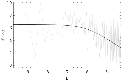
Figure 5: Left panel: histogram of the sample points for parameter $a_{1}$ in Abell 383 coming out the MCMC implementation used to estimate best fit values and errors for our fitting procedure as described in § XI.5. Binning (horizontal axis) and relative frequencies (vertical axis) are given by automatic procedure from Mathematica6.0. Right panel: power spectrum test on sample chain for parameter $a_{1}$ using the method described in § XI.5. Black line is the logarithm of the analytical template Eq. (191) for power spectrum; gray line is the discrete power spectrum obtained using Eq. (189) - (190).

We have run one chain of $10^{5}$ points for every cluster; the convergence of the chains has been tested using the power spectrum analysis from D05 . The key idea of this method is, at the same time, simple and powerful: if we take the power spectra of the MCMC samples, we will have a great correlation on small scales but, when the chain reaches convergence, the spectrum becomes flat (like a white noise spectrum); so that, by checking the spectrum of just one chain (instead of many parallel chains as in Gelmann-Rubin test) will be sufficient to assess the reached convergence. Remanding to D05 for a detailed discussion of all the mathematical steps. Here we calculate the discrete power spectrum of the chains:

$$P_{j}=|a_{N}^{j}|^{2}$$ (189)

with

$$a_{N}^{j}=\frac{1}{\sqrt{N}}\sum_{n=0}^{N-1}x_{n}\exp{\left[i\frac{2\pi j}{N}n\right]}$$ (190)

where $N$ and $x_{n}$ are the length and the element of the sample from the MCMC, respectively, $j=1,\ldots,\frac{N}{2}-1$. The wavenumber $k_{j}$ of the spectrum is related to the index $j$ by the relation $k_{j}=\frac{2\pi j}{N}$. Then we fit it with the analytical template:

$$P(k)=P_{0}\frac{(k^{*}/k)^{\alpha}}{1+(k^{*}/k)^{\alpha}}$$ (191)

or in the equivalent logarithmic form:

$$\ln P_{j}=\ln P_{0}+\ln\left[\frac{(k^{*}/k_{j})^{\alpha}}{1+(k^{*}/k_{j})^{\alpha}}\right]-\gamma+r_{j}$$ (192)

where $\gamma=0.57216$ is the Euler-Mascheroni number and $r_{j}$ are random measurement errors with $<r_{j}>=0$ and $<r_{i}r_{j}>=\delta_{ij}\pi^{2}/6$. From the fit, we estimate the two fundamental parameters, $P_{0}$ and $j^{*}$ (the index corresponding to $k^{*}$). The first one is the value of the power spectrum extrapolated for $k\rightarrow 0$ and, from it, we can derive the convergence ratio from ${\displaystyle r\approx\frac{P_{0}}{N}}$; if $r<0.01$, we can assume that the convergence is reached. The second parameter is related to the turning point from a power-law to a flat spectrum. It has to be $>20$ in order to be sure that the number of points in the sample, coming from the convergence region, are more than the noise points. If these two conditions are verified for all the parameters, then the chain has reached the convergence and the statistics derived from MCMC well describes the underlying probability distribution (typical results are shown in Figs. (2)-(3)). Following D05 prescriptions, we perform the fit over the range $1\leq j\leq j_{max}$, with $j_{max}\sim 10j^{*}$, where a first estimation of $j^{*}$ can be obtained from a fit with $j_{max}=1000$, and then performing a second iteration in order to have a better estimation of it. Even if the convergence is achieved after few thousand steps of the chain, we have decided to run longer chains of $10^{5}$ points to reduce the noise from the histograms and avoid under- or over- estimations of errors on the parameters. The $i-\sigma$ confidence levels are easily estimated deriving them from the final sample the $15.87$-th and $84.13$-th quantiles (which define the $68\%$ confidence interval) for $i=1$, the $2.28$-th and $97.72$-th quantiles (which define the $95\%$ confidence interval) for $i=2$ and the $0.13$-th and $99.87$-th quantiles (which define the $99\%$ confidence interval) for $i=3$.

After the description of the method, let us now comment on the achieved results.

XII Results

The numerical results of our fitting analysis are summarized in Table 2; we give the best fit values of the independent fitting parameters $a_{1}$ and $a_{2}$, and of the gravitational length $L$, considered as a function of the previous two quantities. In Figs. (3)- (5), we give the typical results of fitting, with histograms and power spectrum of samples derived by the MCMC, to assess the reached convergence (flat spectrum at large scales).

The goodness and the properties of the fits are shown in Figs. (6)- (17). The main property of our results is the presence of a typical scale for each cluster above which our model works really good (typical relative differences are less than $5\%$), while for lower scale there is a great difference. It is possible to see, by a rapid inspection, that this turning-point is located at a radius $\approx 150$ kpc. Except for very large clusters, it is clear that this value is independent of the cluster, being approximately the same for any member of the considered sample.

There are two main independent explanations that could justify this trend: limits due to a break in the state of hydrostatic equilibrium or limits in the series expansion of the $f(R)$-models.

If the hypothesis of hydrostatic equilibrium is not correct, then we are in a regime where the fundamental relations Eqs. (169)- (174), are not working. As discussed in Vik05 , the central (70 kpc) region of every cluster is strongly affected by radiative cooling and thus it cannot directly be related to the depth of the cluster potential well. This means that, in this region, the gas is not in hydrostatic equilibrium but in a multi-phase, turbulent state, mainly driven by some astrophysical, non-gravitational interaction. In this case, the gas cannot be used as a good standard tracer.

We have also to consider another limit of our modelling: the requirement that the $f(R)$-function is Taylor expandable. The corrected gravitational potential which we have considered is derived in the weak field limit, which means

$$R-R_{0}<<\frac{a_{1}}{a_{2}}$$ (193)

where $R_{0}$ is the background value of the curvature. If this condition is not satisfied, the approach does not work (see noi-prd for a detailed discussion of this point). Considering that $a_{1}/a_{2}$ has the dimension of $length^{-2}$ this condition defines the length scale where our series approximation can work. In other words, this indicates the limit in which the model can be compared with data.

For the considered sample, the fit of the parameters $a_{1}$ and $a_{2}$, spans the length range $\{19;200\}$ kpc (except for the biggest cluster). It is evident that every galaxy cluster has a proper gravitational length scale. It is worth noticing that a similar situation, but at completely different scales, has been found out for low surface brightness galaxies modelled by $f(R)$-gravity CapCardTro07 .

Considering the data at our disposal and the analysis which we have performed, it is not possible to quantify exactly the quantitative amount of these two different phenomena (i.e. the radiative cooling and the validity of the weak field limit). However, they are not mutually exclusive but should be considered in details in view of a more refined modelling .

Similar issues are present also in Brown06B : they use the the Metric - Skew - Tensor - Gravity (MSTG) as a generalization of the Einstein General Relativity and derive the gas mass profile of a sample of clusters with gas being the only baryonic component of the clusters. They consider some clusters included in our sample (in particular, A133, A262, A478, A1413, A1795, A2029, MKW4) and they find the same different trend for $r\leq 200$ kpc, even if with a different behavior with respect of us: our model gives lower values than X-ray gas mass data while their model gives higher values with respect to X-ray gas mass data. This stresses the need for a more accurate modelling of the gravitational potential.

However, our goal is to show that potential (158) is suitable to fit the mass profile of galaxy clusters and that it comes from a self-consistent theory.

In general, it can be shown that the weak field limit of extended theories of gravity has Yukawa-like corrections b10 ; kenmoku . Specifically, given theory of gravity of order $(2n+2)$, the Yukawa corrections to the Newtonian potential are $n$ Qua91 . This means that if the effective Lagrangian of the theory is

$${\cal L}=f(R,\Box R,..\Box^{k}R,..\Box^{n}R)\sqrt{-g}$$ (194)

we have

$$\phi(r)=-\frac{GM}{r}\left[1+\sum_{k=1}^{n}\alpha_{k}e^{-r/L_{k}}\right]\,.$$ (195)

Standard General Relativity, where Yukawa corrections are not present, is recovered for $n=0$ (second order theory) while the $f(R)$-gravity is obtained for $n=1$ (fourth-order theory). Any $\Box$ operator introduces two further derivation orders in the field equations. This kind of Lagrangian comes out when quantum field theory is formulated on curved spacetime birrell . In the series (195), $G$ is the value of the gravitational constant considered at infinity, $L_{k}$ is the interaction length of the $k$-th component of the non-Newtonian corrections. The amplitude $\alpha_{k}$ of each component is normalized to the standard Newtonian term; the sign of $\alpha_{k}$ tells us if the corrections are attractive or repulsive (see will for details). Moreover, the variation of the gravitational coupling is involved. In our case, we are taking into account only the first term of the series. It is the the leading term. Let us rewrite (158) as

$$\phi(r)=-\frac{GM}{r}\left[1+\alpha_{1}e^{-r/L_{1}}\right]\,.$$ (196)

The effect of non-Newtonian term can be parameterized by $\{\alpha_{1},\,L_{1}\}$ which could be a useful parameterisation which respect to our previous $\{a_{1},\,a_{2}\}$ or $\{G_{eff},\,L\}$ with $G_{eff}=3G/(4a_{1})$. For large distances, where $r\gg L_{1}$, the exponential term vanishes and the gravitational coupling is $G$. If $r\ll L_{1}$, the exponential becomes 1 and, by differentiating Eq.(196) and comparing with the gravitational force measured in laboratory, we get

$$G_{lab}=G\left[1+\alpha_{1}\left(1+\frac{r}{L_{1}}\right)e^{-r/L_{1}}\right]\simeq G(1+\alpha_{1})\,,$$ (197)

where $G_{lab}=6.67\times 10^{-8}$ g^-1cm³s^-2 is the usual Newton constant measured by Cavendish-like experiments. Of course, $G$ and $G_{lab}$ coincide in the standard Newtonian gravity. It is worth noticing that, asymptotically, the inverse square law holds but the measured coupling constant differs by a factor $(1+\alpha_{1})$. In general, any correction introduces a characteristic length that acts at a certain scale for the self-gravitating systems as in the case of galaxy cluster which we are examining here. The range of $L_{k}$ of the $k$th-component of non-Newtonian force can be identified with the mass $m_{k}$ of a pseudo-particle whose effective Compton’s length can be defined as

$$L_{k}=\frac{\hbar}{m_{k}c}\,.$$ (198)

The interpretation of this fact is that, in the weak energy limit, fundamental theories which attempt to unify gravity with the other forces introduce, in addition to the massless graviton, particles with mass which also carry the gravitational interaction gibbons . See, in particular, PPNfelix for $f(R)$-gravity. These masses are related to effective length scales which can be parameterized as

$$L_{k}=2\times 10^{-5}\left(\frac{1\,\mbox{eV}}{m_{k}}\right)\mbox{cm}\,.$$ (199)

There have been several attempts to experimentally constrain $L_{k}$ and $\alpha_{k}$ (and then $m_{k}$) by experiments on scales in the range $1\,\mbox{cm}<r<1000\,\mbox{km}$, using different techniques fischbach ; speake ; eckhardt . In this case, the expected masses of particles which should carry the additional gravitational force are in the range $10^{-13}\mbox{eV}<m_{k}<10^{-5}\,\mbox{eV}$. The general outcome of these experiments, even retaining only the term $k=1$, is that geophysical window between the laboratory and the astronomical scales has to be taken into account. In fact, the range

$$|\alpha_{1}|\sim 10^{-2}\,,\qquad L_{1}\sim 10^{2}\div 10^{3}\,\,\mbox{m}\,,$$ (200)

is not excluded at all in this window. An interesting suggestion has been given by Fujii fujii1 , which proposed that the exponential deviation from the Newtonian standard potential could arise from the microscopic interaction which couples the nuclear isospin and the baryon number.

The astrophysical counterparts of these non-Newtonian corrections seemed ruled out till some years ago due to the fact that experimental tests of General Relativity seemed to predict the Newtonian potential in the weak energy limit, ”inside" the Solar System. However, as it has been shown, several alternative theories seem to evade the Solar System constraints (see PPNfelix ; lecian and the references therein for recent results) and, furthermore, indications of an anomalous, long–range acceleration revealed from the data analysis of Pioneer 10/11, Galileo, and Ulysses spacecrafts (which are now almost outside the Solar System) makes these Yukawa–like corrections come again into play anderson . Besides, it is possible to reproduce phenomenologically the flat rotation curves of spiral galaxies considering the values

$$\alpha_{1}=-0.92\,,\qquad L_{1}\sim 40\,\,\mbox{kpc}\,.$$ (201)

The main hypothesis of this approach is that the additional gravitational interaction is carried by some ultra-soft boson whose range of mass is $m_{1}\sim 10^{-27}\div 10^{-28}$eV. The action of this boson becomes efficient at galactic scales without the request of enormous amounts of dark matter to stabilize the systems sanders .

Furthermore, it is possible to use a combination of two exponential correction terms and give a detailed explanation of the kinematics of galaxies and galaxy clusters, again without dark matter model eckhardt .

It is worthwhile to note that both the spacecrafts measurements and galactic rotation curves indications come from ”outside" the usual Solar System boundaries used up to now to test General Relativity. However, the above results do not come from any fundamental theory to explain the outcome of Yukawa corrections. In their contexts, these terms are phenomenological.

Another important remark in this direction deserves the fact that some authors mcgaugh interpret also the experiments on cosmic microwave background like the experiment BOOMERANG and WMAP Boom ; WMAP in the framework of modified Newtonian dynamics again without invoking any dark matter model.

All these facts point towards the line of thinking that also corrections to the standard gravity have to be seriously taken into account beside dark matter searches.

In our case, the parameters $a_{1,2}$, which determine the gravitational correction and the gravitational coupling, come out "directly" from a field theory with the only requirement that the effective action of gravity could be more general than the Hilbert-Einstein theory $f(R)=R$. This main hypothesis comes from fundamental physics motivations due to the fact that any unification scheme or quantum field theory on curved space have to take into account higher order terms in curvature invariants birrell . Besides, several recent results point out that such corrections have a main role also at astrophysical and cosmological scales. For a detailed discussion, see odi ; capfra ; faraoni .

Figure 6: Density vs $a_{1}$: predictions on the behavior of $a_{1}$. The horizontal black bold line indicates the Newtonian-limit, $a_{1}\rightarrow 3/4$ which we expect to be realized on scales comparable with Solar System. Vertical lines indicate typical approximated values of matter density (without dark matter) for different gravitational structures: Universe (large dashed) with critical density $\rho_{crit}\approx 10^{-26}$ $\mathrm{kg/m^{3}}$; galaxy clusters (short dashed) with $\rho_{cl}\approx 10^{-23}$ $\mathrm{kg/m^{3}}$; galaxies (dot-dashed) with $\rho_{gal}\approx 10^{-11}$ $\mathrm{kg/m^{3}}$; sun (dotted) with $\rho_{sun}\approx 10^{3}$ $\mathrm{kg/m^{3}}$. Arrows and boxes show the predicted trend for $a_{1}$.

With this philosophy in mind, we have plotted the trend of $a_{1}$ as a function of the density in Fig.6. As one can see, its values are strongly constrained in a narrow region of the parameter space, so that $a_{1}$ can be considered a "tracer" for the size of gravitational structures. The value of $a_{1}$ range between $\{0.8\div 0.12\}$ for larger clusters and $\{0.4\div 0.6\}$ for poorer structures (i.e. galaxy groups like MKW4 and RXJ1159). We expect a particular trend when applying the model to different gravitational structures. In Fig. 6, we give characteristic values of density which range from the biggest structure, the observed Universe (large dashed vertical line), to the smallest one, the Sun (vertical dotted line), through intermediate steps like clusters (vertical short dashed line) and galaxies (vertical dot-dashed line). The bold black horizontal line represents the Newtonian limit $a_{1}=3/4$ and the boxes indicate the possible values of $a_{1}$ that we obtain by applying our theoretical model to different structures.

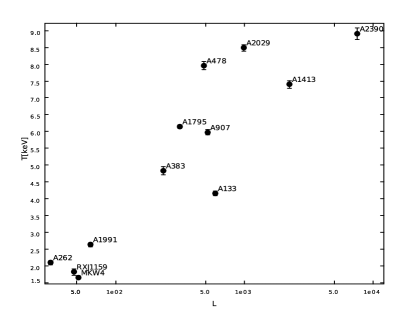
Figure 7: Single temperature fit to the total cluster spectrum (upper panel) and total cluster mass within r₅₀₀ (given as a function of M_⊙) (lower panel) are plotted as a function of the characteristic gravitational length $L$. Temperature and mass values are from Vik06 .

Similar considerations hold also for the characteristic gravitational length $L$ directly related to both $a_{1}$ and $a_{2}$. The parameter $a_{2}$ shows a very large range of variation $\{-10^{6}\div-10\}$ with respect to the density (and the mass) of the clusters. The value of $L$ changes with the sizes of gravitational structure (see Fig. 7), so it can be considered, beside the Schwarzschild radius, a sort of additional gravitational radius. Particular care must be taken when considering Abell 2390, which shows large cavities in the X-ray surface brightness distribution, and whose central region, highly asymmetric, is not expected to be in hydrostatic equilibrium. All results at small and medium radii for this cluster could hence be strongly biased by these effects Vik06 ; the same will hold for the resulting exceptionally high value of $L$. Fig. 7 shows how observational properties of the cluster, which well characterize its gravitational potential (such as the average temperature and the total cluster mass within r₅₀₀, plotted in the left and right panel, respectively), well correlate with the characteristic gravitational length $L$.

For clusters, we can define a gas-density-weighted and a gas-mass-weighted mean, both depending on the series parameters $a_{1,2}$. We have:

$$<L>_{\rho} = 318\;\mathrm{kpc}\qquad<a_{2}>_{\rho}=-3.40\cdot 10^{4}$$

$$<L>_{M} = 2738\;\mathrm{kpc}\qquad<a_{2}>_{M}=-4.15\cdot 10^{5}$$ (202)

It is straightforward to note the correlation with the sizes of the cluster cD-dominated-central region and the "gravitational" interaction length of the whole cluster. In other words, the parameters $a_{1,2}$, directly related to the first and second derivative of a given analytic $f(R)$-model determine the characteristic sizes of the self gravitating structures.

XIII What we have learnt from clusters

We have investigated the possibility that the high observational mass-to-light ratio of galaxy clusters could be addressed by $f(R)$- gravity without assuming huge amounts of dark matter. We point out that this proposal comes out from the fact that, up to now, no definitive candidate for dark-matter has been observed at fundamental level and then alternative solutions to the problem should be viable. Furthermore, several results in $f(R)$-gravity seem to confirm that valid alternatives to $\Lambda$CDM can be achieved in cosmology. Besides, as discussed in the Introduction, the rotation curves of spiral galaxies can be explained in the weak field limit of $f(R)$-gravity. Results of our analysis go in this direction.

We have chosen a sample of relaxed galaxy clusters for which accurate spectroscopic temperature measurements and gas mass profiles are available. For the sake of simplicity, and considered the sample at our disposal, every cluster has been modelled as a self-bound gravitational system with spherical symmetry and in hydrostatic equilibrium. The mass distribution has been described by a corrected gravitational potential obtained from a generic analytic $f(R)$-theory. In fact, as soon as $f(R)\neq R$, Yukawa-like exponential corrections emerge in the weak field limit while the standard Newtonian potential is recovered only for $f(R)=R$, the Hilbert-Einstein theory.

Our goal has been to analyze if the dark-matter content of clusters can be addressed by these correction potential terms. As discussed in detail in the previous sections and how it is possible to see by a rapid inspection of figures, the clusters of the sample are consistent with the proposed model at $1\sigma$ confidence level. This shows, at least qualitatively, that the high mass-to-light ratio of clusters can be explained by using a modified gravitational potential. The good agreement is achieved on distance scales starting from $150$ kpc up to $1000$ kpc. The differences observed at smaller scales can be ascribed to non-gravitational phenomena, such as cooling flows, or to the fact that the gas mass is not a good tracer at this scales. The remarkable result is that we have obtained a consistent agreement with data only using the corrected gravitational potential in a large range of radii. In order to put in evidence this trend, we have plotted the baryonic mass vs radii considering, for each cluster, the scale where the trend is clearly evident.

In our knowledge, the fact that $f(R)$-gravity could work at these scales has been only supposed but never achieved by a direct fitting with data (see fogdm ; lobo for a review). Starting from the series coefficients $a_{1}$ and $a_{2}$, it is possible to state that, at cluster scales, two characteristic sizes emerge from the weak field limit of the theory. However, at smaller scales, e.g. Solar System scales, standard Newtonian gravity has to be dominant in agreement with observations and experiments.

In summary, if our considerations are right, gravitational interaction depends on the scale and the infrared limit is led by the series coefficient of the considered effective gravitational Lagrangian. Roughly speaking, we expect that starting from cluster scale to galaxy scale, and then down to smaller scales as Solar System or Earth, the terms of the series lead the clustering of self-gravitating systems beside other non-gravitational phenomena. In our case, the Newtonian limit is recovered for $a_{1}\rightarrow 3/4$ and $L(a_{1},a_{2})\gg r$ at small scales and for $L(a_{1},a_{2})\ll r$ at large scales. In the first case, the gravitational coupling has to be redefined, in the second $G_{\infty}\simeq G$. In these limits, the linear Ricci term is dominant in the gravitational Lagrangian and the Newtonian gravity is restored Qua91 . Reversing the argument, this could be the starting point to achieve a theory capable of explaining the strong segregation in masses and sizes of gravitationally-bound systems.

Figure 8: As an example of the above results, we have plotted the baryonic mass vs radii for Abell A133. Dashed line is the experimental-observed estimation Eq. (187) of baryonic matter component (i.e. gas, galaxies and cD-galaxy); solid line is the theoretical estimation Eq. (186) for baryonic matter component. Dotted lines are the 1-$\sigma$ confidence levels given by errors on fitting parameters plus statistical errors on mass profiles as discussed in § XI.4 in the right panel.

Figure 9: As the above case, for cluster Abell 383.

Figure 10: As the above cases, for cluster Abell 478.

Figure 11: As the above cases, for cluster Abell 1413.

Figure 12: As the above cases, for cluster Abell 2029.

XIV Conclusions

The present status of art of cosmology shows that the Standard Cosmological Model, based on General Relativity, nucleosynthesis, cosmic abundances and large scale structure, has some evident difficulties. These ones, first of all, rely on some lack of a self-consistent formulation of missing matter and cosmic acceleration issues; such shortcomings give rise to further difficulties in interpreting observational data. With an aphorism, one can say that we have a book, but not the alphabet to read it.

Nowadays there two main philosophical approaches aimed to solve this problem. From one side, there are researchers which try to solve shortcomings of Standard Cosmological Model assuming that General Relativity is right but we need some exotic, invisible kinds of energy and matter to explain cosmic dynamics and large scale structure. On the other side, there are people which believe that General Relativity is not the definitive and comprehensive theory of gravity, and that it should be revised at ultraviolet scales (quantum gravity) and infrared scales (extragalactic and cosmic scales). In the latter case, dark energy and dark matter could be nothing else but the signals that we need a more general theory at large scales, also if General Relativity works very well up to Solar System scales. To some extent, this could be seen as a sort of philosophical debate without solution, but there are possibilities to move the question toward a physical viewpoint.

The $f(R)$-gravity is strictly related to the second point of view. It is a fruitful approach to generalize General Relativity towards the solution also if, most of the models in literature are nothing else but phenomenological models. It is interesting to note that as soon as Einstein formulated his General Relativity, many authors (and Einstein himself) started to explore other possibilities (see capfra for a review). At the beginning, these researches were mainly devoted to check the mathematical consistency of General Relativity but the issues to achieve the unification of gravity with the other interactions (e.g. electromagnetism) pushed several authors to develop alternative gravity theories. Today, one of the goals of alternative gravity is to understand the effective content and dynamics of the Universe. This question is recently become dramatic since assuming that more than 95% of cosmic matter-energy is unknown at fundamental level is highly disturbing. Alternative gravity could be a way out to this situation. The present status of observations, also if we are living in the era of Precision Cosmology, does not allow in discriminating between alternative gravity, from one side, and the presence of dark energy and dark matter, from the other side (the forthcoming LHC experiments should aid in this sense if new fundamental particles will be detected).

However, as discussed in this review, cosmography may be a useful tool to discriminate among different cosmological models being, by definition, a model-independent approach: any cosmographic parameter can be estimated without assigning an a priori cosmological model. So cosmography can be used in two ways:

• One can use it to discriminate between General Relativity and alternative theories. This issue strictly depends on the possibility to have good quality data at disposal. We need some minimum sensibility and error requirements on data surveys to solve this question. At the moment, we have not them and we are not able to do this since standard candles are not available at very high red shifts izzo .

• We can use the cosmographic parameters to constraint cosmological models as we have done in this paper for $f(R)$-gravity. Being these parameters model-independent, they results natural "priors" to any theory. As above, the accuracy in estimating them is a crucial issue.

We have used, essentially, SNeIa but other classes of objects have to be considered in order to improve such an accuracy (e.g. CMBR, bright galaxies, GRBs, BAOs, weak lensing and so on). Forthcoming space missions will be extremely useful in this sense.

Beside cosmography, we have discussed also if $f(R)$-gravity could be useful to address the problem of mass profile and dynamics of galaxy clusters. This issue is crucial in view of achieving any correct model for large scale structure.

Taking into account the weak-field limit of a generic analytic $f(R)$-function, it is possible to obtain a scale-dependent gravity, where scales of self-gravitating systems could naturally emerge. In this way, one could successfully explain dark matter profiles ranging from galaxies to clusters of galaxies. The results are preliminary but seems to indicate a way in which the dark matter puzzle could be completely solved.

In conclusion, the main lesson of this work is that since it is very difficult to discriminate among the huge amount of cosmological models which try to explain the data (deductive approach), it could be greatly fruitful to "reconstruct" the final cosmological model by an inductive approach, that is without imposing it a priori but adopting the philosophy to use the minimum number of parameters . This "inverse scattering approach" could be not fully satisfactory but could lead to self-consistent results.

References

• (1) Alam, U., Sahni, V., Saini, T.D., Starobinsky, A.A., 2003, MNRAS, 344, 1057
• (2) Albrecht et al., Dark energy task force final report, FERMILAB-FN-0793-A, astro-ph/0609591, 2006
• (3) Aldering G. et al., astroโ€‰-โ€‰ph/0405232, 2004; see also snap.lbl.gov
• (4) Allemandi, G., Borowiec, A., Francaviglia, M., 2004, Phys. Rev. D 70, 103503
• (5) Allemandi, G., Francaviglia, M., Ruggiero, M., Tartaglia, A. 2005, Gen. Rel. Grav., 37, 1891
• (6) Anderson J.D., et al., 1998, Phys. Rev. Lett. 81, 2858
• (7) Appleby, S.A., Battye, R.A., 2007, Phys. Lett. B, 654, 7
• (8) ast05 Astier, P. et al. 2006, A&A, 447, 31
• (9) Bahcall N.ย A., 1996, in "Formation of structure in the Universe, 1995, Jerusalem Winter School", astro-ph/9611148,
• (10) Bahcall, N.A. et al. 2003, ApJ, 585, 182
• (11) Bahcall, N.A., Bode, P. 2003, ApJ, 588, 1
• (12) Barris, B.J., et al., 2004, ApJ, 602, 571
• (13) Bautz, L.ย P., Morgan, W.ย W., 1970, ApJ, 162, L149
• (14) Bennett C.L. et al., 2003, ApJS, 148, 1
• (15) Birrell, N.D. and Davies, P.C.W., 1982, Quantum Fields in Curved Space, Cambridge Univ. Press, Cambridge
• (16) Boehmer, C.G., Harko, T., Lobo, F.S.N., 2008, Astropart. Phys. 29, 386
• (17) Borowiec, A., Godlowski, W., Szydlowski, M. 2006, Phys. Rev. D, 74, 043502
• (18) Brownstein, J.ย R., Moffat, J.ย W., 2006, ApJ, 636, 721
• (19) Brownstein, J.ย R., Moffat, J.ย W., 2006, MNRAS, 367, 527
• (20) Brownstein, J.ย R., Moffat, astro-ph/0702146
• (21) Capozziello, S. 2002, Int. J. Mod. Phys. D, 11, 483
• (22) Capozziello, S., Cardone, V.F., Carloni, S., Troisi, A. 2003, Int. J. Mod. Phys. D, 12, 1969
• (23) Capozziello, S., Cardone, V.F., Francaviglia, M. 2006, Gen. Rel. Grav., 38, 711
• (24) Capozziello, S., Cardone, V.F., Troisi, A. 2005, Phys. Rev. D, 71, 043503
• (25) Capozziello, S., Cardone, V.F., Troisi, A. 2006, JCAP, 0608, 001
• (26) Capozziello, S., Cardone, V.ย F., Troisi, A., 2007, MNRAS, 375, 1423
• (27) Capozziello, S., Cardone, V.F., Carloni, S., Troisi, A. 2004, Phys. Lett. A, 326, 292
• (28) Capozziello, S., Cardone, V.F., Elizalde, E., Nojiri, S., Odintsov, S.D., 2006, Phys. Rev. D 73, 043512
• (29) Capozziello, S., Stabile A., Troisi, A., 2007, Class. quant. grav., 24, 2153
• (30) Capozziello, S., Stabile, A., Troisi, A., 2008, Physical Review D, 76, 104019
• (31) Capozziello, S., De Laurentis, M., Nojiri, S., Odintsov, S.D., 2008, arXiv:0808.1335 [hep-th]
• (32) Capozziello, S., Carloni, S., Troisi, A. 2003, Rec. Res. Devel. Astronomy. & Astrophys., 1, 625, astroโ€‰-โ€‰ph/0303041
• (33) Capozziello S. and Francaviglia M., 2008, Gen. Rel. Grav.: Special Issue on Dark Energy 40, 357.
• (34) Capozziello S. and Izzo L., 2008, A&A, 490, 31.
• (35) Capozziello, S., Troisi, A. 2005, Phys. Rev. D, 72, 044022
• (36) Caresia, P., Matarrese, S., Moscardini, L., 2004, ApJ, 605, 21
• (37) Carloni, S., Dunsby, P.K.S., Capozziello, S., Troisi, A. 2005, Class. Quantum Grav. 22, 2839
• (38) Carroll, S.M., Duvvuri, V., Trodden, M., Turner, M.S. 2004, Phys. Rev. D, 70, 043528
• (39) Carroll, S.M., Press, W.H., Turner, E.L. 1992, ARA&A, 30, 499
• (40) Cattoen, C., Visser, M., 2007, Class. Quant. Grav., 24, 5985
• (41) Cembranos, J.A.R. 2006, Phys. Rev. D, 73, 064029
• (42) Chakrabarty, D., de Filippis, E.,& Russell, H.ย 2008, A&A, 487, 75
• (43) Chevallier, M., Polarski, D., 2001, Int. J. Mod. Phys. D, 10, 213
• (44) Chiba, T. 2003, Phys. Lett. B, 575, 1
• (45) Clifton, T., Barrow, J.D. 2005, Phys. Rev. D, 72, 103005
• (46) Clocchiati, A. et al. 2006, APJ, 642, 1
• (47) Cognola, G., Elizalde, E., Nojiri, S., Odintsov, S.D., Sebastiani, L., Zerbini, S., 2008, Phys. Rev. D, 77, 046009
• (48) Cole, S. et al. 2005, MNRAS, 362, 505
• (49) Cooray, A., Huterer, D., Holz, D.E., 2006, Phys. Rev. Lett., 96, 021301
• (50) Copeland E.J., Sami M., Tsujikawa S., 2006, Int. Jou. Mod. Phys. D 15, 1753
• (51) Corasaniti, P.S., LoVerde, M., Crotts, A. et al., 2006, MNRAS, 369, 798
• (52) Croft, R.A.C., Hu, W., Dave, R. 1999, Phys. Rev. Lett., 83, 1092
• (53) de Bernardis, P. et al. 2000, Nature, 404, 955
• (54) de Blok, W.J.G., Bosma, A. 2002, A&A, 385, 816
• (55) de Blok, W.J.G. 2005, ApJ, 634, 227
• (56) De Filippis, E., Sereno, M., Bautz, Longo G., M.ย W., 2005, ApJ, 625, 108
• (57) Dabrowski, M.P., 2005, Phys. Lett. B, 625, 184
• (58) Dabrowski, M.P., Stachowiak, T., 2006, Annals of Physics, 321, 771
• (59) Dabrowski, M.P., 2006, Annalen der Physik, 15, 352
• (60) Davis, T., et al., 2007, ApJ, 666, 716
• (61) Demianski, M., Piedipalumbo, E., Rubano, C., Tortora, C., 2006, A&A, 454, 55
• (62) Dick, R. 2004, Gen. Rel. Grav., 36, 217
• (63) Dodelson S. et al., 2002, ApJ, 572, 140
• (64) Dolgov, A.D., Kawasaki, M. 2003, Phys. Lett. B, 573, 1
• (65) Dunkley, J., Bucher, M., Ferreira, P.ย G., Moodley, K., Skordis, C., 2005, MNRAS, 356, 925
• (66) Dvali, G.R., Gabadadze G., Porrati M., 2000, Phys. Lett. B, 485, 208
• (67) Dvali, G.R., Gabadadze, G., Kolanovic, M., Nitti, F., 2001, Phys. Rev. D, 64, 084004
• (68) Dvali, G.R., Gabadadze, G., Kolanovic, M., Nitti, F., 2002, Phys. Rev. D, 64, 024031
• (69) Eckhardt, D.H., 1993 Phys. Rev. 48 D, 3762.
• (70) Eisenstein, D. et al. 2005, ApJ, 633, 560
• (71) Eke, V.R., Cole, S., Frenk, C.S., Petrick, H.J. 1998, MNRAS, 298, 1145
• (72) Sotiriou, T.P. and Faraoni, V., 2008, arXiv:0805.1726 [gr-qc]
• (73) E. Fischbach, E., Sudarsky, D., Szafer, A., Talmadge, C. and Aroson, S.H., 1986, Phys. Rev. Lett. 56, 3
• (74) Freedman, W.L. et al., 2001, ApJ, 553, 47
• (75) Frieman, J.A., 1997, Comments Astrophys., 18, 323
• (76) Frigerio Martins C. and Salucci P., 2007, Mon.Not.Roy.Astron.Soc. 381, 1103
• (77) Y. Fujii, Y., 1988, Phys. Lett. B 202, 246
• (78) Fujii, I., Maeda, K., The scalarโ€‰-โ€‰tensor theory of gravity, Cambridge University Press, Cambridge (UK), 2003
• (79) Garnavich P.M. et al., 1998, ApJ, 509, 74
• (80) G.W. Gibbons, G.W. and Whiting, B.F., 1981, Nature 291, 636
• (81) Gunnarsson, C., Dahlen, T., Goobar, A., Jรถnsson, J., Mรถrtsell, E., 2006, ApJ, 640, 417
• (82) John, M.V., 2004, ApJ, 614, 1
• (83) John, M.V., 2005, ApJ, 630, 667
• (84) Jรถnsson, J., Dahlen, T., Goobar, A., Gunnarsson, C., Mรถrtsell, E., Lee, K., 2006, ApJ, 639, 991
• (85) Hawkins E. et al., 2003, MNRAS, 346, 78
• (86) Holz, D.E., Wald, R.M., 1998, Phys. Rev. D, 58, 063501
• (87) Holz, D.E., Linder, E.V., 2005, ApJ, 631, 678
• (88) Hu, W., Sawicki, I., 2007, Phys. Rev. D, 76, 064004
• (89) Hui, L., Greene, P.B., 2006, Phys. Rev. D, 73, 123526
• (90) Kaiser N. and the PanSTARRS Team, in Bullettin of the Americal Astronomical Society, page 1049, 2005
• (91) M. Kenmoku, M., Okamoto, Y. and Shigemoto, K., 1993, Phys. Rev. 48 D, 578
• (92) Kim, A.G., Linder, E.V., Miquel, R., Mostek, N., 2004, MNRAS, 347, 909
• (93) Kirkman, D., Tyler, D., Suzuki, N., Oโ€™Meara, J.M., Lubin, D., 2003, ApJS, 149, 1
• (94) Kleinert H., Schmidt, H.-J., 2002, Gen. Rel. Grav. 34, 1295
• (95) Kluske, S., Schmidt, H.J. 1996, Astron. Nachr., 37, 337
• (96) Knop R.A. et al., 2003, ApJ, 598, 102
• (97) Koivisto T., 2007, Phys.Rev.D76, 043527
• (98) Lecian O.M. and Montani G., arXiv:0807.4428 [gr-qc](2008)
• (99) Linder, E.V., 2003, Phys. Rev. Lett., 90, 091301
• (100) Lobo F.S.N., arXiv: 0807.1640[gr-qc] (2008)
• (101) Lue, A., Scoccimarro, R., Starkman, G., 2004, Phys. Rev. D, 69, 044005
• (102) Lue, A., Scoccimarro, R., Starkman, G., 2004, Phys. Rev. D, 69, 124015
• (103) McDonald, P. et al. 2005, ApJ, 635, 761
• (104) S.S. McGaugh, 2000, Ap. J. Lett. 541, L33
• (105) Mendoza S. and Rosas-Guevara Y.M., 2007, Astron.ย Astrophys.ย 472, 367
• (106) Navarro, I., van Acoleyen, K. 2005, Phys. Lett. B, 622, 1
• (107) Netterfield C.B. et al., 2002, ApJ, 571, 604
• (108) Neumann., D.ย M., Bรถhringer, H., 1995, Astron. Astrophys., 301, 865
• (109) Nojiri, S., Odintsov, S.D. 2003, Phys. Lett. B, 576, 5
• (110) Nojiri S., Odintsov, S.D., 2003, Mod. Phys. Lett. A, 19, 627
• (111) Nojiri S., Odintsov, S.D., 2003, Phys. Rev. D, 68, 12352
• (112) Nojiri S. and Odintsov S.D. 2007, Int.ย J.ย Geom.ย Meth.ย Mod.ย Phys.ย 4, 115
• (113) Nojiri, S., Odintsov, S.D., 2007, Phys. Lett. B, 652, 343
• (114) Nojiri, S., Odintsov, S.D., 2007, Phys. Lett. B, 657, 238
• (115) Nojiri S., Odintsov, S.D., Phys. Rev. D accepted (arXiv:0710.1738 [hep-th]) 2007
• (116) Nojiri, S., Odintsov, S. D., arXiv:0801.4843 [astro-ph] 2008
• (117) Nordin, J., Goobar, A., Jรถnsson, J., 2008, JCAP, 02, 008
• (118) Olmo, G.J. 2005, Phys. Rev. D, 72, 083505
• (119) Padmanabhan, T. 2003, Phys. Rept., 380, 235
• (120) Peebles, P.J.E., Rathra, B. 2003, Rev. Mod. Phys., 75, 559
• (121) Percival W.J. et al., 2002, MNRAS, 337, 1068
• (122) Perez Bergliaffa, S.E., 2006, Phys. Lett. B, 642, 311
• (123) Perlmutter S. et al., 1997, ApJ, 483, 565
• (124) Perlmutter S. et al., 1999, ApJ, 517, 565
• (125) Pettorino, V., Baccigalupi, C., Mangano, G., 2005, JCAP, 0501, 014
• (126) Pope, A.C. et al. 2005, ApJ, 607, 655
• (127) Poplawski, N., 2006, Phys. Lett. B, 640, 135
• (128) Poplawski, N., 2007, Class. Quant. Grav., 24, 3013
• (129) Quandt, I., Schmidt H.ย J., 1991, Astron. Nachr., 312, 97
• (130) Rebolo R. et al., 2004, MNRAS, 353, 747
• (131) Refregier, A. 2003, ARA&A, 41, 645
• (132) Riess A.G. et al., 1998, AJ, 116, 1009
• (133) Riess, A.G. et al. 2004, ApJ, 607, 665
• (134) Riess, A.G. et al., 2007, ApJ, 659, 98
• (135) Sahni, V., Starobinski, A. 2000, Int. J. Mod. Phys. D, 9, 373
• (136) Sahni, V., Saini, T.D., Starobinsky, A.A., Alam, U., 2003, JETP Lett., 77, 201
• (137) Sanchez, A.G. et al. 2006, MNRAS, 366, 189
• (138) Sanders, R.H., 1990, Ann. Rev. Astr. Ap. 2, 1
• (139) Sarkar, D., Amblard, A., Holz, D.E., Cooray, A., 2008, ApJ, 678, 1
• (140) Schindler, S., 2004, Astrophys.Space Sci., 28, 419
• (141) Schmidt B.P. et al., 1998, ApJ, 507, 46
• (142) Schmidt, H.J. 2004, Lectures on mathematical cosmology, grโ€‰-โ€‰qc/0407095
• (143) Schmidt, R.ย W., Allen S.ย W., 2007 MNRAS 379, 209
• (144) Schmidt, B.P., Keller, S.C., Francis P.J. et al., Bullettin of the Americal Astronomical Society, 37, 457, 2005
• (145) Seljak, U. et al. 2005, Phys. Rev. D, 71, 103515
• (146) Sobouti, Y. 2007, A & A, 464, 921
• (147) Sotiriou, T.P. 2006, Gen. Rel. Grav., 38, 1407
• (148) Speake, C.C. and Quinn, T.J., 1988, Phys. Rev. Lett. 61, 1340
• (149) Spergel, D.N. et al. 2003, ApJS, 148, 175
• (150) Spergel, D.N. et al., 2007, ApJS, 170, 377
• (151) Starobinsky, A.A., 2007, JETP Lett., 86, 157
• (152) Stelle, K., 1978, Gen. Relat. Grav., 9, 353
• (153) Stompor R. et al., 2001, ApJ, 561, L7
• (154) Szalay A.S. et al., 2003, ApJ, 591, 1
• (155) The Dark Energy Survey Collaboration, astroโ€‰-โ€‰ph/0510346, 2005
• (156) Tegmark, M. et al. 2004, Phys. Rev. D, 69, 103501
• (157) Tegmark M. et al., 2006, Phys. Rev. D, 74, 123507
• (158) Tegmark, M., Taylor, A.N., Heavens, A.F., 2007, ApJ, 4802, 22
• (159) Tonry J.L. et al., 2003, ApJ, 594, 1
• (160) Tsujikawa, S., 2008, Phys. Rev. D 77, 023507
• (161) Tyson, J.A. in Survey and Other Telescope Technologies and Discoveries, ed. J.A. Tyson and S.Wolff, page 10, Sidney, 2002
• (162) van Waerbecke, L. et al. 2001, A&A, 374, 757
• (163) Viana, P.T.P., Nichol, R.C., Liddle, A.R. 2002, ApJ, 569, 75
• (164) Vikhlinin, A., Markevitch, M., Murray, S.ย S., Jones, C., Forman, W., Van Speybroeck, L., 2005, ApJ, 628, 655
• (165) Vikhlinin, A., Kravtsov, A., Forman, W., Jones, C., Markevitch, M., Murray, S.ย S., Van Speybroeck, L., 2006, ApJ, 640, 691
• (166) Visser, M., 2004, Class. Quant. Grav., 21, 2603
• (167) Wambsganss, J., Cen, R., Gu, X., Ostriker, J.P., 1997, ApJ, 475, L81
• (168) Wang, Y., ApJ, 536, 531
• (169) Wang, Y., Mukherejee, P., 2004, ApJ, 606, 654
• (170) Weinberg, S., Gravitation and cosmology, Wiley, New York, 1972
• (171) Will C.M., 1993, Theory and Experiments in Gravitational Physics, Cambridge Univ. Press, Cambridge.
• (172) Woodโ€‰-โ€‰Vasey, W.M., et al., 2007, ApJ, 666, 694
• (173) Zwicky, F., 1933, Helv. Phys. Acta, 6, 110