Spherical volume averages of static electric and magnetic fields using Coulomb and Biot-Savart laws

Abstract

We present derivations of the expressions for the spherical volume averages of static electric and magnetic fields that are virtually identical. These derivations utilize the Coulomb and Biot-Savart laws, and make no use of vector calculus identities or potentials.

I Introduction

The average of static electric or magnetic fields over a sphere has been used to obtain important results, such as the macroscopic electric field inside a dielectricgriffiths and the presence of $\delta$-function electric (magnetic) fields at the position of electric (magnetic) point dipoles.jackson In both electric and magnetic cases, if the sources of the fields are outside the averaging sphere, the average field equals the value of the field at the center of the sphere, whereas for sources inside the averaging sphere, the average electric and magnetic fields are proportional to the electric and magnetic dipole moments of the sources, respectively.

Textbooks typically only treat the electric field case.electric_only Only a handful of authors jackson ; both treat both electric and magnetic cases, probably because the magnetic field case is considered to be “tough” by undergraduate standards,griffiths1 since the derivations typically employ the magnetic vector potential and vector calculus identities. This paper presents derivations of both the electric and magnetic field cases that are virtually identical and are elementary, in the sense that they rely on Coulomb’s and the Biot-Savart laws and make no use of vector calculus identities or potentials.

Coulomb’s law states that the electric field for a unit point charge is

$${\bm{G}}(\bm{r})=k\frac{\bm{r}}{r^{3}},$$ (1)

where $\bm{r}$ is a displacement vector from the point charge, $r=|\bm{r}\,|$ and $k=(4\pi\epsilon_{0})^{-1}$ and $1$ in SI and Gaussian units, respectively. In terms of $\bm{G}$, the electric field the electric field ${\bm{E}}$ at point $\bm{s}$ due to a static charge distribution $\rho(\bm{r}^{\prime})$ is

$$\bm{E}(\bm{s}) =\int d\bm{r}^{\prime}\ \rho(\bm{r}^{\prime})\,\bm{G}(\bm{s}-\bm{r}^{\prime})=-\int d\bm{r}^{\prime}\ \rho(\bm{r}^{\prime})\,\bm{G}(\bm{r}^{\prime}-\bm{s}).$$ (2)

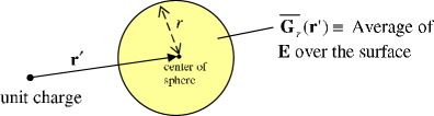
Figure 1: Definition of $\overline{\bm{G}}_{r}(\bm{r}^{\prime})$: the average of the electric field of a unit charge about a spherical surface of radius $r$, centered at $\bm{r}^{\prime}$ relative to the charge.

Define $\overline{\bm{G}_{r}}(\bm{r}^{\prime})$ to be the average of $\bm{G}$ over a spherical surface of radius $r$ around a point $\bm{r}^{\prime}$, as shown in Fig. 1. An apparently little-known result that is critical in following discussion is (see the appendix for derivations)

$$\overline{\bm{G}_{r}}(\bm{r}^{\prime})=k\frac{\bm{r}^{\prime}}{r^{\prime 3}}\;\Theta(r^{\prime}-r)$$ (3)

where $\Theta$ is the Heavyside step function.heavyside Eq. (3) implies that the average of the electric field over the surface of the sphere for a point charge outside the sphere ($r^{\prime}>r$) equals the electric field at the center of the sphere, whereas a point charge inside a sphere ($r^{\prime}<r$) contributes zero to the average of the electric field over the surface of the sphere. In a sense, this result is the antithesis of the integral form of Gauss’ law,difference but it is not as general as Gauss’ law because it applies only to spherical surfaces.

II Volume averages of static electric fields

Let $\langle\bm{E}\rangle_{R}$ to be average of the electric field $\bm{E}$ about a spherical volume of radius $R$ and $\overline{\bm{E}_{r}}(\bm{0})$ be the average electric field over a spherical shell of radius $r$, both centered around the origin. Then,

$$\langle\bm{E}\rangle_{R} \equiv \frac{3}{4\pi R^{3}}\int_{r=0}^{R}\!d{\bm{r}}\ \bm{E}(\bm{r})=\frac{3}{R^{3}}\int_{0}^{R}dr\ r^{2}\;\overline{\bm{E}_{r}}(\bm{0}).$$ (4)

For a given charge distribution $\rho(\bm{r}^{\prime})$, $\overline{\bm{E}_{r}}(\bm{0})$ can be obtained by setting $\bm{s}=\bm{0}$ and averaging both sides of Eq. (2) over a spherical shell of radius $r$, yielding

$$\overline{\bm{E}_{r}}(\bm{0}) =-\int d\bm{r}^{\prime}\ \rho(\bm{r}^{\prime})\,\overline{\bm{G}_{r}}(\bm{r}^{\prime}).$$ (5)

II.1 Single point charge

We first examine the case of a single point charge. Because electric fields obey the principle of linear superposition, what holds for a single point charge is generalizable to cases of many charges and/or continuous charge distributions. Substituting the charge distribution for a point charge $q$ at $\bm{d}$, $\rho(\bm{r}^{\prime})=q\,\delta(\bm{r}^{\prime}-\bm{d})$, into Eq. (5) gives $\overline{\bm{E}_{r}}(\bm{0})=-q\overline{\bm{G}_{r}}(\bm{d})$. Substituting this into Eq. (4) and using Eq. (3) gives

$$\langle\bm{E}\rangle_{R}=-\frac{3kq\bm{d}}{d^{3}R^{3}}\int_{0}^{R}dr\ r^{2}\;\Theta(d-r).$$ (6)

If the point charge is outside the averaging sphere of radius $R$, then $d>R$ and the integral in Eq. (6) equals $R^{3}/3$. Hence, $\langle\bm{E}\rangle_{R}^{\rm(out)}=-kq\bm{d}/d^{3}=\bm{E}(\bm{0})$, the electric field at the center of the sphere due to the point charge. On the other hand, if the point charge is inside the averaging sphere, then $d<R$ and the integral in Eq. (6) equals $d^{3}/3$, in which case $\langle\bm{E}\rangle^{\rm(in)}_{R}=-k\bm{p}/R^{3}$, where $\bm{p}=q\bm{d}$ is the dipole moment of the point charge relative to the center of the sphere.

II.2 Arbitrary charge distribution

We now obtain these results more rigorously for an arbitrary charge distribution $\rho(\bm{r}^{\prime})$. Substituting Eqs. (3) and (5) into Eq. (4) yields,

$$\langle{\bm{E}}\rangle_{R} =-\frac{3}{R^{3}}\int_{0}^{R}dr\ r^{2}\left[\int_{r^{\prime}=r}^{\infty}d\bm{r}^{\prime}\ \frac{k\,\rho(\bm{r}^{\prime})\;\bm{r}^{\prime}}{r^{\prime 3}}\right].$$ (7)

where the effect of the $\Theta$ function in Eq. (3) is to restrict the $\bm{r}^{\prime}$ integration to the region $|\bm{r}^{\prime}|>r$. We now consider separately the contribution of the charges outside and inside the sphere.

II.2.1 Sources outside the sphere

The contribution due to charges outside the sphere of radius $R$ corresponds to $\int_{r^{\prime}=R}^{\infty}d\bm{r}^{\prime}$ in Eq. (7), which makes the term in square parentheses independent of $r$. The integration over $r$ gives $R^{3}/3$, yielding

$$\langle\bm{E}\rangle^{\rm(out)}_{R}=-\int_{r^{\prime}=R}^{\infty}\!d\bm{r}^{\prime}\ \frac{k\,\rho(\bm{r}^{\prime})\;\bm{r}^{\prime}}{r^{\prime 3}}=\bm{E}^{\rm(out)}(\bm{0})$$ (8)

the electric field at the origin. Therefore, in general, $\langle\bm{E}\rangle_{R}^{\rm(out)}=\bm{E}^{\rm(out)}$ at the center of the sphere.

II.2.2 Sources inside the sphere

Sources inside the sphere of radius $R$ correspond to $|\bm{r}^{\prime}|<R$ in Eq. (7). This gives

$$\langle\bm{E}\rangle_{R}^{\rm(in)} =-\frac{3}{R^{3}}\int_{0}^{R}dr\ r^{2}\int_{r^{\prime}=r}^{R}d\bm{r}^{\prime}\ \frac{k\,\rho(\bm{r}^{\prime})\;\bm{r}^{\prime}}{r^{\prime 3}}$$

$$=-\frac{3k}{R^{3}}\int_{r^{\prime}=0}^{R}d\bm{r}^{\prime}\ \frac{\rho(\bm{r}^{\prime})\;\bm{r}^{\prime}}{r^{\prime 3}}\int_{0}^{r^{\prime}}dr\ r^{2}$$

$$=-\frac{k}{R^{3}}\int_{r^{\prime}=0}^{R}d\bm{r}^{\prime}\;\rho(\bm{r}^{\prime})\;{\bm{r}^{\prime}}=-\frac{k\,\bm{p}}{R^{3}},$$ (9)

where $\bm{p}=\int d\bm{r}^{\prime}\ \rho(\bm{r}^{\prime})\,\bm{r}^{\prime}$ is the dipole moment relative to the center of the sphere, and we have used $\int_{0}^{R}dr\int_{r}^{R}dr^{\prime}=\int_{0}^{R}dr^{\prime}\int_{0}^{r^{\prime}}dr$, as shown in Fig. 2.

III Magnetic field case

A static magnetic field $\bm{B}$ is related to the charge current density $\bm{J}$ by the Biot-Savart law,

$$\bm{B}(\bm{s})=\int d\bm{r}^{\prime}\ \bm{J}(\bm{r}^{\prime})\bm{\times}\bm{G}(\bm{s}-\bm{r}^{\prime}),$$ (10)

where $k=\mu_{0}/(4\pi)$ or $c^{-1}$ for SI or gaussian, respectively. Comparison of Eq. (10) with Eq. (2) shows that the derivation for the magnetic field case can be copied wholesale from the electric field case by substituting $\bm{E}\rightarrow\bm{B}$ and $\rho\rightarrow\bm{J}\bm{\times}$ at every step. (The only point of caution is that the cross product anti-commutes, so care must be taken to preserve the order of $\bm{J}$ and $\overline{\bm{G}}$ or $\bm{r}^{\prime}$.) Using these substitutions in Eq. (8) gives, for current sources outside the averaging sphere,

$$\langle\bm{B}\rangle_{R}^{\rm(out)} =-\int_{r^{\prime}=R}^{\infty}d\bm{r}^{\prime}\ \frac{k\,\bm{J}(\bm{r}^{\prime})\times\bm{r}^{\prime}}{r^{\prime 3}}=\bm{B}(\bm{0}),$$ (11)

the magnetic field at the center of the sphere. For current sources inside the averaging sphere, using the substitutions in Eq. (9) gives

$$\langle\bm{B}\rangle_{R}^{\rm(in)} =-\frac{k}{R^{3}}\int_{r^{\prime}=0}^{R}d\bm{r}^{\prime}\bm{J}(\bm{r}^{\prime})\times{\bm{r}^{\prime}}=\frac{\,2k\bm{m}}{R^{3}},$$ (12)

where $\bm{m}=\frac{1}{2}\int d\bm{r}^{\prime}\ \bm{r}^{\prime}\bm{\times}\bm{J}(\bm{r}^{\prime})$ is the magnetic dipole moment.jackson1

Appendix A Derivation of Eq. (3)

By definition,

$$\overline{\bm{G}_{r}}(\bm{r}^{\prime})=\frac{1}{4\pi r^{2}}\int dA^{\prime\prime}\ \bm{G}(\bm{r}^{\prime\prime}),$$ (13)

where the integral is over the spherical shell of radius $r$ around $\bm{r}^{\prime}$. Choose $\bm{r}^{\prime}=r^{\prime}\hat{\bm{z}}$, where $\hat{\bm{z}}$ is the unit vector in the $z$-direction. By azimuthal symmetry, $\overline{\bm{G}_{r}}(r^{\prime}\hat{\bm{z}})=\overline{G_{r}}_{,z}\hat{\bm{z}}=(4\pi r^{2})^{-1}\int dA^{\prime\prime}\,G_{z}(\bm{r}^{\prime\prime})\hat{\bm{z}}$, where $G_{z}$ is the $z$-component of $\bm{G}$. By dividing the spherical surface into strips $dA^{\prime\prime}=r^{2}\sin\theta\,d\theta$ (see Fig. 3), $\overline{G_{r}}_{,z}=\frac{1}{2}\int_{0}^{\pi}d\theta\ \sin\theta\ G_{z}(\bm{r}^{\prime\prime})$. Letting $\mu=\cos\theta$, and using $G_{z}(\bm{r}^{\prime\prime})=kr_{z}^{\prime\prime}/|\bm{r}^{\prime\prime}|^{3}$ gives

$$\overline{G_{r}}_{,z} =\frac{k}{2}\int_{-1}^{1}d\mu\ \frac{r\mu+r^{\prime}}{(r^{2}+r^{\prime 2}+2r^{\prime}r\mu)^{3/2}}$$

$$=-\frac{k}{2}\frac{\partial}{\partial r^{\prime}}\left[\int_{-1}^{1}d\mu\ \frac{1}{(r^{2}+r^{\prime 2}+2r^{\prime}r\mu)^{1/2}}\right]$$

$$=-\frac{k}{2}\frac{\partial}{\partial r^{\prime}}\left[\frac{\sqrt{r^{2}+r^{\prime 2}+2r^{\prime}r\mu}}{r^{\prime}r}\right]_{\mu=-1}^{1}=-\frac{k}{2}\frac{\partial}{\partial r^{\prime}}\left[\frac{|r+r^{\prime}|-|r-r^{\prime}|}{r^{\prime}r}\right]$$

$$=\begin{cases}{-\displaystyle k\,\frac{\partial r^{-1}}{\partial r^{\prime}}=0}&\mbox{for $r^{\prime}<r$};\\ \vspace{-0.6cm}\\ {-\displaystyle k\,\frac{\partial r^{\prime-1}}{\partial r^{\prime}}=\frac{k}{r^{\prime 2}}}&\mbox{for $r^{\prime}>r$},\end{cases}$$ (14)

which implies Eq. (3).

This result can also be obtained by using the well known property that the average of an electrostatic potential of a point charge $Q$ over the surface of a sphere of radius $r$ equals the potential at the center if the charge is outside the sphere, and $Q/(4\pi\epsilon_{0}r)$ if the charge is inside.griffiths2 Stated mathematically, if $V(\bm{r}^{\prime\prime})=k/|\bm{r}^{\prime\prime}|$, then the average of $V$ over a spherical shell of radius $r$ around $\bm{r}^{\prime}$ is

$$\overline{V_{r}}(\bm{r}^{\prime})=k\begin{cases}r^{\prime-1}&\mbox{for $|\bm{r}^{\prime}|>r$};\\ r^{-1}&\mbox{for $|\bm{r}^{\prime}|<r$}.\end{cases}$$ (15)

Averaging over spherical shells on both sides of the relation $\bm{G}(\bm{r}^{\prime})=-\nabla^{\prime}V(\bm{r}^{\prime})$ yields $\overline{\bm{G}_{r}}(\bm{r}^{\prime})=-\nabla^{\prime}\,\overline{V_{r}}(\bm{r}^{\prime})$. Using Eq. (15) in this gives Eq. (3).

Figures

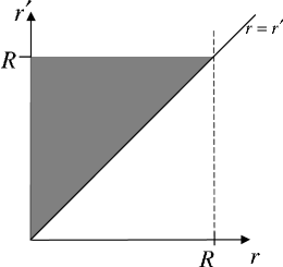
Figure 2: Integration region for the limits $\int_{0}^{R}dr\int_{r}^{R}dr^{\prime}$ (grey region). Integration over this region can also be written as $\int_{0}^{R}dr^{\prime}\int_{0}^{r^{\prime}}dr.$

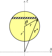
Figure 3: Spherical surface over which $G_{z}$ is averaged to obtain $\overline{G_{r}}_{,z}$. The hatched strip indicates the area element $dA^{\prime\prime}$ on the sphere with constant $G_{z}(\theta)=kr_{z}^{\prime\prime}/|\bm{r}^{\prime\prime}|^{3}$ where $r^{\prime\prime}_{z}=r^{\prime}+r\cos\theta$ and $|\bm{r}^{\prime\prime}|=\sqrt{r^{\prime 2}+r^{2}+2rr^{\prime}\cos\theta}$.

References

- (1) David J. Griffiths, Introduction to Electrodynamics (Prentice-Hall, New Jersey, 1999) 3rd ed., pp. 173 – 175.
- (2) John D. Jackson, Classical Electrodynamics (Wiley, New York, 1999) 3rd ed., pp. 148 – 150 and pp. 187 – 188.
- (3) See e.g., Wolfgang Pauli, Electrodynamics (MIT Press, Cambridge, MA, 1973) pp. 37-39; Paul Lorrain, Dale P. Corson, and François Lorrain, Electromagnetic Fields and Waves (W. H. Freeman, New York, 1988) 3rd ed., pp. 56-57; B. K. P. Scaife, Principles of Dielectrics (Oxford University Press, Oxford, 1989), appendix F; Evaristo Riande and Ricardo D az-Calleja, Electrical Properties of Polymers (Marcel Dekker, New York, 2004) p. 44; Saunak Palit, Principles of Electricity and Magnetism (Alpha Science International, Harrow, U.K., 2005) pp. 61-63; Tai L. Chow, Introduction to Electromagnetic Theory: A Modern Perspective (Jones and Bartlett, Boston, 2006) p. 86, problem 9.
- (4) See, e.g., Ref. griffiths, , pp. 156 – 157, p. 253 and David J. Griffiths, Instructor’s Solutions Manual: Introduction to Electrodynamics (Prentice Hall, Englewood Cliffs, NJ, 1999), pp. 108 – 109; A. Z. Capri and P. V. Panat, Introduction to Electrodynamics (Narosa, New Delhi, 2002), pp. 155-158 and pp. 242-246; Ben Yu-Kuang Hu, “Averages of static electric and magnetic fields over a spherical region: A derivation based on the mean-value theorem,” Am. J. Phys. 68, 1058–1060 (2000).
- (5) Ref. griffiths, , p. 253, problem 5.57.
- (6) The Heavyside function is defined to be for , for and .
- (7) Note the difference between the average of a vector field over a surface , (where is the area of surface ), and the flux of through the surface, (where is a unit vector perpendicular to area element ). This paper deals with the former, while Gauss’ law pertains to the latter.
- (8) See e.g., Ref. griffiths, , p. 254; Ref. jackson, , p. 186.
- (9) See e.g., Ref. griffiths, , pp. 114 – 115.