Intersecting branes and Nambu$-$Jona-Lasinio model

Abstract

We discuss chiral symmetry breaking in the intersecting brane model of Sakai and Sugimoto at weak coupling for a generic value of separation $L$ between the flavour $D8$ and anti-$D8$-branes. For any finite value of the radius $R$ of the circle around which the colour $D4$-branes wrap, a non-local Nambu$-$Jona-Lasinio (NJL) type short-range interaction couples the flavour branes and anti-branes. We argue that chiral symmetry is broken in this model only above a certain critical value of the $4$-dimensional ’t Hooft coupling and confirm this through numerical calculations of solutions to the gap equation. We also numerically investigate chiral symmetry breaking in the limit $R\rightarrow\infty$ keeping $L$ fixed, but find that simple ways of implementing this limit do not lead to a consistent picture of chiral symmetry breaking in the non-compact version of the non-local NJL model.

Contents

1. 1 Introduction
2. 2 NJL model from QCD
   1. 2.1 Extension to a non-local NJL model
3. 3 NJL model from weakly coupled SS model
   1. 3.1 Non-local NJL from SS model
4. 4 $\chi$SB in non-local NJL model
   1. 4.1 Gap equation and order parameter of $\chi$SB
   2. 4.2 Solutions of the gap equation
   3. 4.3 Numerical solutions
5. 5 The non-compact limit
6. 6 Summary

1 Introduction

The Nambu$-$Jona-Lasinio (NJL) model [2] provides an example of dynamical chiral symmetry breaking ($\chi$SB) and fermion mass generation in a simple effective field theory setting. In the original model, the fermions in the four-fermi interaction were taken to be the nucleons. Interest in the model has endured for two main reasons: (i) It appears to give a rather accurate description of chiral symmetry breaking and its consequences for low-energy hadron phenomenology; (ii) Appropriately replacing the original nucleons by coloured quarks, the model can be argued to describe all of the low-energy physics of QCD, including the anomaly term [3, 4, 5] .

Recently, versions of the NJL model have emerged in a string theory setting [7, 8], involving intersecting brane configurations. One such configuration is the model of Sakai and Sugimoto (SS) [9], which involves a system of intersecting $D4$, $D8$ and anti-$D8$-branes. The SS model has been very successful in reproducing many of the qualitative features of non-abelian chiral symmetry breaking in QCD. In this model, the ‘colour’ Yang-Mills fields are provided by the massless open string fluctuations of a stack of $N_{c}$ $D4$-branes, which are extended along the four space-time directions and in addition wrap a thermal circle of radius $R$. At scales much larger than string length, the theory on the $D4$-branes is $(4+1)$-dimensional pure Yang-Mills with coupling $g_{5}^{2}=(2\pi)^{2}g_{s}l_{s}$ of length dimension. In the strong coupling limit, $g_{5}^{2}N_{c}>>2\pi R$, this stack of $D4$-branes has a dual description in terms of a classical gravity theory [10] with the background geometry of a Euclidean black hole. Flavour degrees of freedom [11, 12, 13] are provided by the massless open string fluctuations between the colour branes and the ‘flavour’ $D8$ and anti-$D8$-branes, which intersect the thermal circle at points separated by a distance $L\leq\pi R$. Various aspects of chiral symmetry breaking in this model have been discussed in [9, 14, 7, 8, 15, 16, 17, 18, 19, 20, 21, 22, 23, 24, 25, 26, 27, 28, 29, 30, 31, 32].

It was pointed out in [7] that the brane configuration of the SS model decouples the scales of chiral symmetry breaking and confinement . The additional parameter in the SS model (as compared to QCD) which makes this possible is the ratio $L/R$. The authors of [7] argued that in the limit $R\rightarrow\infty$ with $L$ kept fixed (non-compact SS model), the effective low-energy description of the SS model at weak coupling is given by a non-local version of the NJL model, which breaks chiral symmetry spontaneously at arbitrarily weak coupling. This result is surprising in view of our field theoretic intuition, which would suggest that chiral symmetry is not broken at weak coupling and that there is a transition to the broken phase at some critical value. One might suspect that this unexpected result is connected with the absence of a mass gap in the non-compact SS model, which results in a long-range four-fermi interaction. One way to test this hypothesis would be to work with a finite, but possibly very large, value of $R$, which corresponds to a confining theory with possibly a small, but non-zero, mass gap. From general arguments, one would expect chiral symmetry to be broken in this model at a length scale of the order of or smaller than the confinement scale . However, in the corresponding effective non-local NJL model which describes the flavour brane-antibrane interactions, $\chi$SB could be associated with length scales even larger than the confinement scale. This is because the NJL model does not incorporate confinement. Now, the point is that for solutions which have $\chi$SB scale larger than the confinement scale, an effective local NJL model should be adequate. But this latter model shows a critical coupling for $\chi$SB. This argument suggests that an effective non-local NJL model for the SS model would show $\chi$SB only beyond a critical value of the coupling.

In this paper we analyze $\chi$SB at weak coupling in the brane configuration of the SS model, with a finite value of $R$ and a generic value of $L$. This theory has a mass gap, which gives the scale over which the four-fermi coupling of the flavour branes extends. We obtain the leading order (in gauge coupling) approximation to the effective fermion action, including the exact contribution due to the Kaluza-Klein modes. We expand on the plausibility argument given above that in the resulting non-local NJL model chiral symmetry is spontaneously broken only above a certain critical coupling. We then verify this by obtaining numerical solutions to the gap equation derived from the effective fermi theory. The plan of this paper is as follows. In the next section we first briefly review the argument of [4] for the emergence of local NJL model from QCD and then extend it to a non-local model. We use this in Section 3 to derive the non-local NJL model as the leading approximation to the coupling of the flavour branes in the weakly coupled SS model. In Section 4, we discuss $\chi$SB in the non-local NJL model. We derive the gap equation in the large $N_{c}$ limit and present numerical solutions which show that chiral symmetry is spontaneously broken only above a certain critical coupling. A discussion of the non-compact case is given in Section 5. We end with a summary in Section 6.

2 NJL model from QCD

The Yang-Mills action for $U(N_{c})$ gauge group (indices $a,b$) and $N_{f}$ massless quark flavours (indices $\alpha,\beta$) is

$$S_{0}=-\frac{1}{4g_{4}^{2}}\int d^{4}x\ (F_{\mu\nu}^{a}(x))^{2}+\int d^{4}x\ {\bar{q}}^{\alpha}(x)\gamma^{\mu}\biggl{(}i\partial_{\mu}+t^{a}A^{a}_{\mu}(x)\biggr{)}q^{\alpha}(x).$$ (1)

This theory confines and develops a mass scale $\Lambda$, given by

$$\Lambda\sim m\ e^{-\frac{1}{\beta_{0}g_{4}^{2}}},\qquad\beta_{0}=\frac{1}{24\pi^{2}}(11N_{c}-2N_{f}).$$ (2)

It is generally believed that at energies below the confining scale, an effective NJL model for quarks captures the dynamics of the theory. There is no systematic way of integrating out the Yang-Mills degrees of freedom from QCD to get an effective fermion action. A scenario outlining how one might think about doing this was presented in [4]. The basic point is that integration of Yang-Mills degrees of freedom would lead to effective multi-quark interactions. The range of these interactions must be short, of the order of $1/\Lambda$, because of confinement, and so at energies below $\Lambda$ a local approximation would be adequate. The NJL interaction between gauge-invariant quark bilinears is the leading term compatible with gauge symmetry and global symmetries of QCD.

2.1 Extension to a non-local NJL model

In QCD it is generally believed that the mass scale $M$ associated with $\chi$SB coincides with the confinement scale $\Lambda$. Suppose, however, we can deform QCD in such a way that the two scales are separated by some new physics (as in the SS intersecting brane configuration discussed in the next section). In this case, for studying $\chi$SB we need the effective four-fermi theory at energies larger than the mass gap $\Lambda$. If $\Lambda<<M$, the energies of quarks involved in the four-fermi interaction are much larger than $\Lambda$. Because of asymptotic freedom, for energies much larger than $\Lambda$ we can present a more precise derivation of the effective interaction. The leading contribution to the effective interaction comes from a one-gluon exchange approximation, which can be calculated exactly. The result is

$$S_{0~{}{\rm eff}}=-\frac{g_{4}^{2}}{2}\int d^{4}x\ d^{4}y\ \Delta_{0}(x-y)\ J^{a\mu}(x)J^{a}_{\mu}(y)$$ (3)

where

$$J^{a\mu}(x)=\biggl{(}q^{\dagger}_{L}(x){\bar{\sigma}}^{\mu}t^{a}q_{L}(x)+q^{\dagger}_{R}(x)\sigma^{\mu}t^{a}q_{R}(x)\biggr{)},$$ (4)

and

$$\Delta_{0}(x)=\int\frac{d^{4}k}{(2\pi)^{4}}\frac{e^{ik.x}}{{\bar{k}}^{2}},\qquad{\bar{k}}^{2}\equiv{\vec{k}}^{2}-k_{0}^{2}-i\epsilon.$$ (5)

is the Feynman propagator for a massless scalar . Using the Fierz identities given in equations (3.77) and (3.80) of [34] and retaining only interaction terms between left and right-handed Weyl components , the effective action (3) becomes

$$S_{0~{}{\rm eff}}=g_{4}^{2}\int d^{4}x\ d^{4}y\ \Delta_{0}(x-y)[q^{\dagger\alpha}_{L}(x)q^{\beta}_{R}(y)][q^{\dagger\beta}_{R}(y)q^{\alpha}_{L}(x)],$$ (6)

The bilocal fermion products in square brackets are singlets of the (global) colour $U(N_{c})$ group and transform as $({\bar{N}_{f}},N_{f})$ under the flavour $U(N_{f})\times U(N_{f})$ group.

The above discussion may be summarized as follows. The effective four-fermi theory resulting from integrating out the gluon degrees of freedom is

$$S_{0~{}{\rm eff}} = i\int\ d^{4}x\biggl{(}q^{\dagger\alpha}_{L}(x){\bar{\sigma}}^{\mu}\partial_{\mu}q^{\alpha}_{L}(x)+q^{\dagger\alpha}_{R}(x)\sigma^{\mu}\partial_{\mu}q^{\alpha}_{R}(x)\biggr{)}$$ (7)

$$+g_{4}^{2}\int d^{4}x\ d^{4}y\ G_{0}(x-y)[q^{\dagger\alpha}_{L}(x)q^{\beta}_{R}(y)][q^{\dagger\beta}_{R}(y)q^{\alpha}_{L}(x)],$$

where

$$G_{0}(x)=\int\frac{d^{4}k}{(2\pi)^{4}}\ e^{ik.x}\ \tilde{G}_{0}(k),$$ (8)

$\tilde{G}_{0}(k)$ satisfies:

• For ${\bar{k}}<<\Lambda$, $\tilde{G}_{0}(k)\sim$ constant. This is ensured by the property of confinement of the action (1), which leads to the generation of a mass gap. The constant has length dimension two and we may take it to be $1/\Lambda^{2}$. In a sense, this provides a definition of the mass scale $\Lambda$ for us.

• For $\Lambda<<{\bar{k}}<<M$, $\tilde{G}_{0}(k)\sim 1/{\bar{k}}^{2}$. This follows from the asymptotic freedom property of the action (1) and the added new physics which separates the $\chi$SB scale from the mass gap of (1).

A simple example of a function $\tilde{G}_{0}(k)$ which satisfies these two properties is

$$\tilde{G}_{0}(k)=\frac{1}{{\bar{k}}^{2}+\Lambda^{2}}.$$ (9)

A cut-off scale of order $M$ on (9) is understood. A more complicated function could be devised to take into account the running of the coupling. In any case, the process of integrating out gluon degrees of freedom in a confining theory is expected to give rise to a far more complicated effective fermion action than in the model given by (7), (8) and (9). However, one might hope that the essential features for studying qualitative questions about $\chi$SB are present in this model. In the next section, we will see that a very similar non-local NJL interaction between the flavour branes emerges as the leading approximation to the weakly coupled SS model.

3 NJL model from weakly coupled SS model

At scales much smaller than the string length, the dynamics of the weakly coupled SS model is governed by the action

$$S = -\frac{1}{4g_{5}^{2}}\int d^{4}x\int_{0}^{2\pi R}\ dx^{4}\ (F_{MN}^{a}(x,x^{4}))^{2}+\int\ d^{4}x\ q^{\alpha\dagger}_{L}(x){\bar{\sigma}}^{\mu}\biggl{(}i\partial_{\mu}+t^{a}A^{a}_{\mu}(x,-L/2)\biggr{)}q^{\alpha}_{L}(x)$$ (10)

$$\hskip 113.81102pt+\int\ d^{4}x\ q^{\alpha\dagger}_{R}(x)\sigma^{\mu}\biggl{(}i\partial_{\mu}+t^{a}A^{a}_{\mu}(x,L/2)\biggr{)}q^{\alpha}_{R}(x).$$

Only the space-time components $A_{\mu}(x,\mp L/2)$ of the $(4+1)$-dimensional $U(N_{c})$ gauge field $A_{M}(x,x^{4})$ interact with the massless Weyl fermions $q^{\alpha}_{L,R}(x)$. Substituting the Kaluza-Klein expansion

$$A^{a}_{M}(x,x^{4})=A_{M}^{a(0)}(x)+\sum_{n=1}^{\infty}\biggl{(}A_{M}^{a(n)}(x)e^{inx^{4}/R}+{A_{M}^{a(n)}}^{*}(x)e^{-inx^{4}/R}\biggr{)}$$ (11)

in this action, we get

$$S=S_{0}+S_{1}+\cdots$$ (12)

$S_{0}$ becomes identical to the action (1), after identifying the gauge potential $A^{a}_{\mu}(x)$ of the latter with the zero mode $A^{a(0)}_{\mu}(x)$ and setting

$$g_{4}^{2}=g_{5}^{2}/2\pi R.$$ (13)

Also, it is now natural to identify the mass scale $m$ in (2) with $1/\pi R$ since the $4$-dimensional description breaks down beyond this scale. $S_{1}$ is given by

$$S_{1} = \frac{1}{g_{4}^{2}}\sum_{n=1}^{\infty}\int d^{4}x\biggl{(}-\frac{1}{2}|\partial_{\mu}A_{\nu}^{a(n)}(x)-\partial_{\nu}A_{\mu}^{a(n)}(x)|^{2}+\frac{n^{2}}{R^{2}}|A_{\mu}^{a(n)}(x)|^{2}\biggr{)}$$ (14)

$$+\sum_{n=1}^{\infty}\int\ d^{4}x\biggl{(}{J_{n}^{a\mu}}^{*}(x)A_{\mu}^{a(n)}(x)+J_{n}^{a\mu}(x){A_{\mu}^{a(n)}}^{*}(x)\biggr{)},$$

where we have used the notation

$$J_{n}^{a\mu}(x)=\biggl{(}q^{\dagger}_{L}(x){\bar{\sigma}}^{\mu}t^{a}q_{L}(x)e^{inL/2R}+q^{\dagger}_{R}(x)\sigma^{\mu}t^{a}q_{R}(x)e^{-inL/2R}\biggr{)}.$$ (15)

The dots in (12) represent cubic and quartic interactions of the gauge fields. These will not be relevant to the leading order analysis in the weak coupling limit discussed below.

We have already discussed the integration of the massless gluon degrees of freedom from the action $S_{0}$. Integrating out the massive Kaluza-Klein modes from the action (14) is a much simpler task. To leading order in the gauge coupling, the effective four-fermi interaction due to the exchange of these modes is given by

$$S_{1~{}{\rm eff}}=-g_{4}^{2}\sum_{n=1}^{\infty}\int d^{4}x\ d^{4}y\ \Delta_{n}(x-y){J_{n\mu}^{a}}^{*}(x)J_{n}^{a\mu}(y),$$ (16)

where

$$\Delta_{n}(x-y)=\int\frac{d^{4}k}{(2\pi)^{4}}\frac{e^{ik.(x-y)}}{({\bar{k}}^{2}+\frac{n^{2}}{R^{2}})},\qquad{\bar{k}}^{2}\equiv{\vec{k}}^{2}-k_{0}^{2}-i\epsilon.$$ (17)

is the Feynman propagator for a scalar of mass $\frac{n}{R}$. Using the Fierz identities (3.77) and (3.80) of [34] and, as before, retaining only interaction terms between left and right-handed Weyl components, the effective action (16) becomes

$$S_{1~{}{\rm eff}}=2g_{4}^{2}\int d^{4}x\ d^{4}y\biggl{(}\sum_{n=1}^{\infty}\cos(\frac{nL}{R})\Delta_{n}(x-y)\biggr{)}[q^{\dagger\alpha}_{L}(x)q^{\beta}_{R}(y)][q^{\dagger\beta}_{R}(y)q^{\alpha}_{L}(x)].$$ (18)

Now, using the identity 1.445.2 of [35],

$$\sum_{n=1}^{\infty}\frac{\cos ns}{n^{2}+a^{2}}=\frac{\pi}{2a}\frac{\cosh a(\pi-s)}{\sinh\pi a}-\frac{1}{2a^{2}}\ ,$$

we get

$$S_{1~{}{\rm eff}}=g_{4}^{2}\int d^{4}x\ d^{4}y\ G_{1}(x-y)[q^{\dagger\alpha}_{L}(x)q^{\beta}_{R}(y)][q^{\dagger\beta}_{R}(y)q^{\alpha}_{L}(x)],$$ (19)

where

$$G_{1}(x)=\int\frac{d^{4}k}{(2\pi)^{4}}\ e^{ik.x}\ \tilde{G}_{1}(k),\qquad\tilde{G}_{1}(k)=\frac{\pi R\cosh{\bar{k}}(\pi R-L)}{{\bar{k}}\sinh{\bar{k}}\pi R}-\frac{1}{{\bar{k}}^{2}}.$$ (20)

A few comments are in order:

• The interaction in (19), (20) is exact for all values of $L$ and $R$, since we have summed over the exchange of all the Kaluza-Klein modes. In particular, in the limit $R\rightarrow\infty$, keeping $L$ fixed, we get

  $$\tilde{G}_{1}(k)\rightarrow\frac{\pi R}{\bar{k}}e^{-{\bar{k}}L}.$$ (21)

• For finite $R$, howsoever large, the second term in $\tilde{G}_{1}(k)$ cancels the singularity in the first term in the limit ${\bar{k}}<<1/\pi R$. This is consistent with our expectation that the range of the effective interaction (19) should be of order the Kaluza-Klein radius $R$. In fact, for fermion momenta much smaller than $1/R$, one can approximate this non-local interaction by a local NJL term, with small derivative corrections.

• For ${\bar{k}}>>1/L$, the second term on the right hand side in (20) dominates, giving rise to a potentially problematic short-distance interaction with a ‘wrong’ sign. However, this term is cancelled by the large $\bar{k}$ contribution to the total effective action coming from the zero mode action, (5) and (6). The net result is that for $\bar{k}>>1/L$, $G_{1}(k)$ has the behaviour given in (21).

3.1 Non-local NJL from SS model

Combining (19) with (7), we get the total effective fermion action

$$S_{\rm eff} = i\int\ d^{4}x\biggl{(}q^{\dagger\alpha}_{L}(x){\bar{\sigma}}^{\mu}\partial_{\mu}q^{\alpha}_{L}(x)+q^{\dagger\alpha}_{R}(x)\sigma^{\mu}\partial_{\mu}q^{\alpha}_{R}(x)\biggr{)}$$ (22)

$$+g_{4}^{2}\int d^{4}x\ d^{4}y\ G(x-y)[q^{\dagger\alpha}_{L}(x)q^{\beta}_{R}(y)][q^{\dagger\beta}_{R}(y)q^{\alpha}_{L}(x)],$$

where

$$G(x) = \int\frac{d^{4}k}{(2\pi)^{4}}\ e^{ik.x}\ \tilde{G}(k),$$ (23)

and $\tilde{G}(k)=\tilde{G}_{0}(k)+\tilde{G}_{1}(k)$. Although a precise derivation of $\tilde{G}_{0}(k)$ does not exist, it must satisfy certain conditions which we discussed in the previous section. As a result of these, $\tilde{G}(k)$ must satisfy:

• For ${\bar{k}}\sim\Lambda$, $\tilde{G}(k)\sim 1/(k^{2}+\Lambda^{2})$. This follows from the hierarchy of scales $\Lambda<<1/\pi R\leq 1/L$ and the fact that the range of the non-local quartic fermion interaction in (22) is set by the mass gap dynamically generated in the $4$-dimensional Yang-Mills action (1), which is of order the glueball mass $\sim\Lambda$.

• For $\Lambda<<{\bar{k}}<<1/\pi R$, $\tilde{G}(k)\sim 1/{\bar{k}}^{2}$. This is because for these values of $\bar{k}$, the $4$-dimensional description continues to be valid and we are in the asymptotically free regime.

• For ${\bar{k}}>>1/\pi R$, $\tilde{G}(k)\sim\pi Re^{-{\bar{k}}L}/{\bar{k}}$. Here we have assumed $L<<\pi R$ (which is automatically satisfied in the limit of large $R$, keeping $L$ fixed). In this regime, the $4$-dimensional description is inadequate since the Kaluza-Klein states can be easily excited. We must now use the full $5$-dimensional description. The exponential fall-off implies that the quartic fermion interaction in (22) has a short-distance cut-off as well. The effective scale here is of order $L$, the separation between flavour $D8$ and anti-$D8$-branes.

A simple function that contains all the three scales and seems to capture all the essential features discussed above is

$$\tilde{G}(k)=\biggl{(}\frac{1+\pi R\bar{k}}{\bar{k}^{2}+\Lambda^{2}}\biggr{)}e^{-{\bar{k}}L}.$$ (24)

This differs from (9) in that $1/L$ enters as a smooth ultraviolet scale, as opposed to the hard cut-off $M$ that came with (9). Moreover, it contains the additional scale $R$, which has to do with the underlying $5$-dimensional origin of the model. We will use this simpler function in the analysis that follows. Also, throughout the following we will assume $L<<\pi R$.

4 $\chi$SB in non-local NJL model

As usual, we first introduce scalars to rewrite (22) in the equivalent form

$$S_{\rm eff} = i\int\ d^{4}x\biggl{(}q^{\dagger\alpha}_{L}(x){\bar{\sigma}}^{\mu}\partial_{\mu}q^{\alpha}_{L}(x))+q^{\dagger\alpha}_{R}(x)\sigma^{\mu}\partial_{\mu}q^{\alpha}_{R}(x)\biggr{)}$$ (25)

$$+\int d^{4}x\int d^{4}y\biggl{[}-\frac{{T^{\alpha\beta}}^{*}(x,y)T^{\alpha\beta}(x,y)}{g_{4}^{2}G(x-y)}+{T^{\alpha\beta}}^{*}(x,y)q^{\dagger\beta}_{R}(y)q^{\alpha}_{L}(x)$$

$$\hskip 113.81102pt+T^{\alpha\beta}(x,y)q^{\dagger\alpha}_{L}(x)q^{\beta}_{R}(y)\biggr{]}.$$

It is easy to verify the equivalence of this action to (22) by using the equations of motion of the scalars,

$$T^{\alpha\beta}(x,y)=g_{4}^{2}\ G(x-y)\ q^{\dagger\beta}_{R}(y)q^{\alpha}_{L}(x).$$ (26)

The next step is to integrate out the fermions to get an effective action for the scalars. In the large-$N_{c}$ limit, a classical treatment is adequate. Since we are only interested in the solution corresponding to the ground state, which is Poincare invariant and invariant under diagonal (vector) flavour group, we may use the ansatz $T^{\alpha\beta}(x,y)=\delta^{\alpha\beta}T(|x-y|)$. This simplifies calculation of the effective action. Making a Wick rotation to the Euclidean signature, we get

$$\frac{S^{E}_{\rm eff}}{VN_{c}N_{f}}=\frac{1}{g_{4}^{2}N_{c}}\int d^{4}x\ \frac{|T(x)|^{2}}{G^{E}(x)}-\int\frac{d^{4}k}{(2\pi)^{4}}\ {\rm ln}\biggl{(}1+\frac{|\tilde{T}(k)|^{2}}{k^{2}}\biggr{)},$$ (27)

where $V$ is the $4$-volume and $\tilde{T}(k)$ is related to $T(x)$ by a Fourier transform, which we define by the relation (8) for any function. Also, $G^{E}(x)$ is the Euclidean version of $G(x)$. Taking the Fourier transform of (24), we get

$$G^{E}(x)=\frac{1}{4\pi^{2}|x|}\int_{0}^{\infty}dk\ k^{2}J_{1}(k|x|)\biggl{(}\frac{1+\pi Rk}{k^{2}+\Lambda^{2}}\biggr{)}e^{-kL},$$ (28)

where $k$ is the magnitude of the Euclidean four-momentum and $J_{1}(k|x|)$ is a standard Bessel function. The $k$-integral can be done using the identity

$$\frac{1+\pi Rk}{k^{2}+\Lambda^{2}}=\frac{1+i\pi R\Lambda}{2i\Lambda}\int_{0}^{\infty}ds\ e^{is\Lambda}\ e^{-sk}+c.c.,$$ (29)

and the identity 6.623.2 of [35]. After some simplification, the final expression takes the form

$$G^{E}(x)=\frac{\Lambda^{2}}{4\pi^{2}}\ g(|x|\Lambda),$$ (30)

where

$$g(r)=\frac{R_{\Lambda}}{(L_{\Lambda}^{2}+r^{2})^{3/2}}+(\cos L_{\Lambda}+R_{\Lambda}\sin L_{\Lambda})\ \mathcal{I}_{1}(r)+(\sin L_{\Lambda}-R_{\Lambda}\cos L_{\Lambda})\ \mathcal{I}_{2}(r).$$ (31)

In the above, we have introduced the dimensionless quantities

$$R_{\Lambda}=\pi R\Lambda,\qquad L_{\Lambda}=L\Lambda.$$ (32)

Moreover,

$$\mathcal{I}_{1}(r) = \int^{\infty}_{L_{\Lambda}}ds\frac{\cos s}{(s^{2}+r^{2})^{3/2}}=\frac{K_{1}(r)}{r}-\int^{L_{\Lambda}}_{0}ds\frac{\cos s}{(s^{2}+r^{2})^{3/2}},$$

$$\mathcal{I}_{2}(r) = \int^{\infty}_{L_{\Lambda}}ds\frac{\sin s}{(s^{2}+r^{2})^{3/2}}=\frac{1}{r}-\frac{\pi}{2r}(I_{1}(r)-\mathbf{L}_{1}(r))-\int^{L_{\Lambda}}_{0}ds\frac{\sin s}{(s^{2}+r^{2})^{3/2}},$$ (33)

where $K_{1}(r)$ and $I_{1}(r)$ are standard Bessel functions and $\mathbf{L}_{1}(r)$ is a Struve function. It turns out that numerical calculations are done faster with the second form of $\mathcal{I}_{1,2}(r)$. Note that in the region $r<<R_{\Lambda}$, all the $5$ dimensions must come into play. Indeed, in this region we get

$$g(r)\approx\left\{\begin{array}[]{rcl}R_{\Lambda}/L_{\Lambda}^{3}&\mbox{for}&r<<L_{\Lambda}\\ R_{\Lambda}/r^{3}&\mbox{for}&L_{\Lambda}<<r<<R_{\Lambda}\end{array}\right.$$ (36)

For $r>>R_{\Lambda}$, the system becomes effectively $4$-dimensional. Here we find

$$g(r)\approx\left\{\begin{array}[]{rcl}1/r^{2}&\mbox{for}&1>>r>>R_{\Lambda}\\ \sqrt{\frac{\pi}{2}}e^{-r}/r^{3/2}&\mbox{for}&r>>1\end{array}\right.$$ (39)

Figure 1: $g(r)$ as a function of $r$ for the parameter values $L_{\Lambda}=0.01$ and $R_{\Lambda}=0.2$.

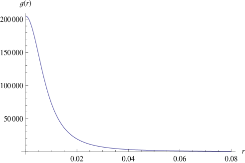
In Figure 1 we have plotted the function $g(r)$ as a function of $r$. We see that it approaches a constant for $r<<L_{\Lambda}$. For $r\gtrsim L_{\Lambda}$, it decreases very rapidly and eventually for $r>1$ (far beyond the region shown in the figure) it decays exponentially .

4.1 Gap equation and order parameter of $\chi$SB

The equation of motion for $T(x)$ following from the effective action (27) is

$$\frac{1}{g_{4}^{2}N_{c}}\int d^{4}x\ \frac{T(x)}{G^{E}(x)}e^{-ik.x}=\frac{\tilde{T}(k)}{k^{2}+|\tilde{T}(k)|^{2}}$$ (40)

This nonlinear equation for the order parameter is the analogue of the gap equation for the present case. $T(x)=0$ is the trivial solution which preserves chiral symmetry. However, this is not the solution which minimizes the effective action (27). To see this [7], multiply (40) on both sides by $\tilde{T}^{*}(k)$ and integrate over $k$. This gives

$$\frac{1}{g_{4}^{2}N_{c}}\int d^{4}x\ \frac{|T(x)|^{2}}{G^{E}(x)}=\int\frac{d^{4}k}{(2\pi)^{4}}\frac{|\tilde{T}(k)|^{2}}{k^{2}+|\tilde{T}(k)|^{2}}.$$ (41)

Using this in (27), we get

$$\frac{S^{E}_{\rm eff}}{VN_{c}N_{f}}=\int\frac{d^{4}k}{(2\pi)^{4}}\biggl{[}\frac{|\tilde{T}(k)|^{2}}{k^{2}+|\tilde{T}(k)|^{2}}-{\rm ln}\biggl{(}1+\frac{|\tilde{T}(k)|^{2}}{k^{2}}\biggr{)}\biggr{]},$$ (42)

It is easy to see that the integrand on the right-hand side above is a decreasing function of $|\tilde{T}(k)|/k$ and that it vanishes for $\tilde{T}(k)=0$. It follows that $\tilde{T}(k)=0$ is not the solution which minimizes the effective action (27). We also note that a potential divergence from the large $k$ end gets cancelled between the two terms in the integrand and the net result of the integration over $k$ is finite, provided $\tilde{T}(k)$ is a decreasing function for large $k$. If such a solution exists, then the chiral symmetry is spontaneously broken.

The order parameter of chiral symmetry breaking is the condensate

$$\phi(x)=\frac{1}{N_{c}}\langle q^{\dagger\alpha}_{L}(x)q^{\alpha}_{R}(0)\rangle.$$ (43)

The field $T(x)$ is related to it by (26), i.e.

$$T(x)=4\pi^{2}\lambda\ G^{E}(x)\ \phi(x),\qquad\lambda\equiv g_{4}^{2}N_{c}/4\pi^{2}.$$ (44)

The gap equation (40) can be rewritten in terms of $\phi(x)$ as

$$\tilde{\phi}(k)=\frac{\tilde{T}(k)}{k^{2}+|\tilde{T}(k)|^{2}}.$$ (45)

We will look for solutions of this equation with $\phi(x)$, and hence $T(x)$, real. Since these are spherically symmetric functions of $|x|$, their Fourier transforms, $\tilde{\phi}(k)$ and $\tilde{T}(k)$, are also real functions of $k$. Furthermore, we see from (45) that for large $k$, $\tilde{\phi}(k)<<1/k$. This is because $\tilde{T}(k)$ must be a decreasing function for large $k$, for reasons explained above. Now, solving (45) for $\tilde{T}(k)$ as a function of $\tilde{\phi}(k)$, we get

$$\tilde{T}_{\pm}(k)=\frac{1}{2\tilde{\phi}(k)}\biggl{[}1\pm\sqrt{1-4k^{2}\tilde{\phi}^{2}(k)}\biggr{]}.$$ (46)

This has real solutions only for $\tilde{\phi}(k)\leq 1/2k$. For large $k$, with $\tilde{\phi}(k)<<1/k$, we get $\tilde{T}_{+}(k)>>k$ and $\tilde{T}_{-}(k)<<k$. So, the desired solution $\tilde{T}(k)$ must coincide with $\tilde{T}_{-}(k)$ for large $k$. For small enough $k$, the solution $\tilde{T}(k)$ must go to a constant (the mass gap) and so it must coincide with $\tilde{T}_{+}(k)$ for small $k$. The transition from one to the other occurs at some scale $k=\mu$, where the two solutions coincide, i.e. $\tilde{T}_{+}(\mu)=\tilde{T}_{-}(\mu)$. From (46) we see that $\mu$ satisfies the equation $\tilde{\phi}(\mu)=1/2\mu$.

4.2 Solutions of the gap equation

We parametrise the condensate as follows:

$$\phi(x)=\frac{\phi_{0}}{4\pi^{2}l^{3}}\varphi(|x|/l).$$ (47)

Here $l$ is the $\chi$SB scale. The normalization has been chosen to explicitly display the dimensions of the order parameter and to have $\varphi(0)=1$. Now, using (44), the Fourier transforms, $\tilde{\phi}(k)$ and $\tilde{T}(k)$, can be written as

$$\tilde{\phi}(k)=l\phi_{0}\ f(kl),\qquad\quad~{}f(p)\equiv\frac{1}{p}\int^{\infty}_{0}dy\ y^{2}J_{1}(py)\ \varphi(y),$$

$$\tilde{T}(k)=\lambda l_{\Lambda}\Lambda\phi_{0}\ t(kl),\qquad t(p)\equiv\frac{1}{p}\int^{\infty}_{0}dy\ y^{2}J_{1}(py)\ g(l_{\Lambda}y)\ \varphi(y),$$ (48)

where $l_{\Lambda}\equiv l\Lambda$ and $J_{1}$ is a standard Bessel function. Using these, we can rewrite the gap equation (45) as

$$f(p)=\frac{\bar{\lambda}t(p)}{p^{2}+\bar{\lambda}^{2}\phi_{0}^{2}t^{2}(p)},\qquad\bar{\lambda}\equiv\lambda l_{\Lambda}.$$ (49)

This is a nonlinear equation which we are unable to solve analytically. However, there are some general observations we can make.

• Equation (49) cannot have a solution with the $\chi$SB scale $l$ arbitrarily smaller than $L$. On physical grounds, we expect $\varphi(|x|/l)$ to be substantially different from zero only in the region $0\leq|x|\lesssim l$, vanishing rapidly for $|x|>>l$. As a result, most of the contribution to the integral in the definition of $t(p)$ in (48) comes from a region in which the argument of the function $g(r)$ varies over the range $[0,l_{\Lambda}]$. For $l<<L$, $g(r)$ is roughly a constant ($=\frac{R_{\Lambda}}{L_{\Lambda}^{3}}$) over this range of $r$, as can be seen from (31). So, for $l<<L$, $t(p)\approx\frac{R_{\Lambda}}{L_{\Lambda}^{3}}f(p)$. But this is not a solution to (49), as can be easily checked. This argument works even better for large $p$, because then the contribution to the integral from $y>1$ region is even more suppressed, beyond that due to a rapidly falling $\varphi(y)$. But, for large $p$ a solution to (49) must satisfy $t(p)\propto p^{2}f(p)$. Thus, the gap equation (49) has no solutions for $l<<L$.

• In principle, $\chi$SB solutions to the gap equation should exist for all $l\geq L$. This is because our non-local NJL model does not incorporate confinement. However, for solutions which have $l>\Lambda^{-1}$, i.e. $l_{\Lambda}>1$, it should be possible to replace the non-local model by an effective local NJL model with $\Lambda$ as the ultraviolet cut-off. This is because of the exponential decay of the four-fermi interaction $g(r)$ for $r>1$. Since the local NJL model has no $\chi$SB solutions below a critical coupling, we expect a critical coupling to show up for values of order $l_{\Lambda}\gtrsim 1$ in the present non-local NJL model as well. One way this can happen is that as $l_{\Lambda}$ increases beyond $L_{\Lambda}$, the value of $\lambda$ which gives rise to this solution decreases until it hits a critical value at around $l_{\Lambda}\sim 1$. This argument cannot be made for the non-compact SS model considered in [7] because of the absence of the mass scale $\Lambda$ and the consequent absence of the exponential decay of $g(r)$ for $r>1$.

Numerical calculations reported below bear out both the above expectations.

4.3 Numerical solutions

In the following, we will report on some solutions to the gap equation (49) obtained numerically using mathematica. This numerical work is based on the following strategy. From the expected physical properties of the order parameter $\phi(x)$, we first make an ansatz for it:

$$\varphi(x)=\frac{e^{-x}}{(c^{2}x^{2}+1)^{\sigma}}.$$ (50)

The power $\sigma$ and the constant $c$ are adjustable parameters. With the $\chi$SB scale $l$ and the normalization constant $\phi_{0}$, there are altogether four adjustable parameters. Given (50), the two sides of (49) can be computed and compared, and the difference can be minimized by varying these parameters. The numerical computations were done as follows. For the left-hand side of (49), we need to calculate $f(p)$. This can be done once we choose some values for $\sigma$ and $c$. After some experience with the calculations, it was not hard to make a good guess for the right values. For the right-hand side of (49), we need $t(p)$ for which one first needs to calculate the function $g(r)$. This requires choosing values for $R_{\Lambda}$ and $L_{\Lambda}$. In Figure 1 we have shown an example of $g(r)$ for $R_{\Lambda}=0.2$ and $L_{\Lambda}=0.01$. With $g(r)$ at hand, one can now calculate $t(p)$, after making a choice for $l_{\Lambda}$. The right-hand-side of (49), which we denote as $f_{t}(p)$,

$$\frac{\bar{\lambda}t(p)}{p^{2}+\bar{\lambda}^{2}\phi_{0}^{2}t^{2}(p)}\equiv f_{t}(p),$$ (51)

can then be computed. This requires making a choice for the parameters $\bar{\lambda}$ and $\phi_{0}$, which are adjusted such that the deviation $\int dp(f(p)-f_{t}(p))^{2}$ is minimized. In principle, in the calculation of the deviation, the range of the integral over $p$ should extend to infinity. In practice, we have found a value of about $10$ to be good enough for the upper limit (for the values of the parameters $L_{\Lambda}$ and $R_{\Lambda}$ we have used in our calculations), in the sense that the value of the integral remains essentially unchanged if the upper limit is increased beyond this value. The whole procedure was then repeated with slightly different values of $\sigma$, $c$, $\bar{\lambda}$ and $\phi_{0}$ until the deviation was minimized for the chosen values of $R_{\Lambda}$, $L_{\Lambda}$ and $l_{\Lambda}$. The value of $\lambda$ relevant to these values of the parameters was obtained from its relation to $\bar{\lambda}$ given in (49).

Figure 2: The functions $f(p)$ and $f_{t}(p)$ shown in these figures are the two sides of the gap equation. The two figures correspond to two different sets of values of $\{R_{\Lambda},L_{\Lambda}\}$, as indicated.

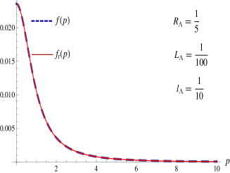
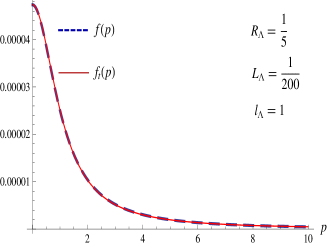
In Figure 2 we have given two examples of the quality of solutions obtained in this way for two different sets of values of $\{R_{\Lambda},L_{\Lambda}\}$, with $l_{\Lambda}>>L_{\Lambda}$. The agreement between $f(p)$ and $f_{t}(p)$ is excellent. In fact, the deviation $\int dp(f(p)-f_{t}(p))^{2}$ is less than a thousandth of a percent of the quantity $\int dp(f(p))^{2}$. Surprisingly, in all the solutions that we have obtained, the value of the parameter $c$ which minimizes the deviation turns out to be exactly $l/L$. This may provide a hint for analytical solutions of the gap equation.

Note that both cases in Figure 2 have $l_{\Lambda}>>L_{\Lambda}$. As argued in the previous subsection, we do not expect any solution for $l_{\Lambda}<<L_{\Lambda}$. In fact, our numerical calculations indicate that there is no solution for $l_{\Lambda}\lesssim L_{\Lambda}$.

Figure 3: The two sides of the gap equation for $l_{\Lambda}=L_{\Lambda}/5$.

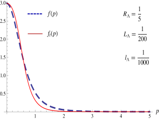
This can be seen from the example given in Figure 3 where we have taken $l_{\Lambda}=L_{\Lambda}/5$. There is no agreement, which is the best we have been able to do with the ansatz (50). The seeming agreement at large $p$ is misleading because the values of both $f(p)$ and $f_{t}(p)$ are so small that the figure cannot distinguish them from zero at the scale used.

Figure 4: The first figure shows $t(p)/f(p)$ for $l_{\Lambda}<L_{\Lambda}$ and the second figure shows $p^{2}f(p)/t(p)$ for $l_{\Lambda}>>L_{\Lambda}$ as a function of $p$.

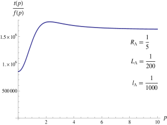
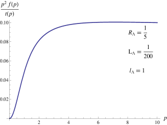
A better measure for the behaviour at large $p$ is the ratio $t(p)/f(p)$, which is expected to approach a constant at large $p$ for $l_{\Lambda}<<L_{\Lambda}$. In the first of Figure 4 we have plotted this ratio. It behaves as predicted at large $p$. The value of the constant also turns out to be close to the expected one, namely $R_{\Lambda}/L_{\Lambda}^{3}$. For comparison, in the second of Figure 4 we have plotted the ratio $p^{2}f(p)/t(p)$ for the second example of Figure 2, which is expected to approach a constant at large $p$ since this provides a solution to the gap equation. The figure verifies this, implying that in this case $t(p)\sim p^{2}f(p)$ at large $p$.

In Figure 5 we have plotted $l_{\Lambda}$ as a function of $\lambda$. Figures for two different sets of values of $\{R_{\Lambda},L_{\Lambda}\}$ have been given.

Figure 5: $l_{\Lambda}$ as a function of $\lambda$ for two different sets of values of $\{R_{\Lambda},L_{\Lambda}\}$.

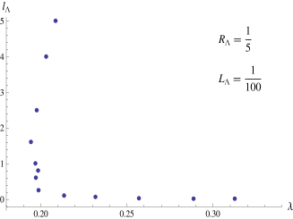
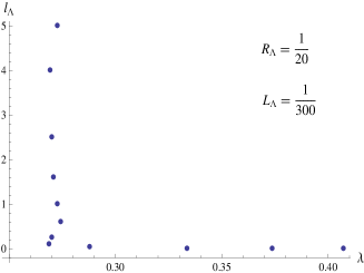
Starting with $l_{\Lambda}=L_{\Lambda}$, we see that at first $\lambda$ decreases with increasing $l_{\Lambda}$, until it reaches a minimum at around $l_{\Lambda}=1$. Beyond this point, increasing $l_{\Lambda}$ seems to be accompanied by an unchanged or perhaps even an increasing $\lambda$ . We have verified the behaviour shown in the two examples in Figure 5 for several other values of the set $\{R_{\Lambda},L_{\Lambda}\}$ and believe that this is the general behaviour. These data provide fairly convincing evidence for the existence of a critical value of $\lambda$ below which no solutions to the gap equation exist.

5 The non-compact limit

It is of interest to ask what happens in the non-compact limit, $R\rightarrow\infty$ keeping $L$ fixed. In our model, taking this limit is somewhat subtle, because the hierarchy of scales $L<<\pi R<<\Lambda^{-1}$ must be maintained as the limit is taken. Furthermore, even though the non-local NJL model does not incorporate confinement, to connect with the underlying weakly coupled gauge theory we may wish to impose on this model the relations between the confinement scale $\Lambda^{-1}$, $R$ and the coupling $g_{5}^{2}$, given by (2) and (13) (with $m\sim 1/\pi R$). Under the scaling $R\rightarrow R(\eta)=\eta R$, the following scaling properties can be deduced from these relations:

$$R_{\Lambda}(\eta)=(R_{\Lambda})^{\eta},\qquad L_{\Lambda}(\eta)=L_{\Lambda}\frac{(R_{\Lambda})^{\eta-1}}{\eta},$$ (52)

where $L_{\Lambda}$ and $R_{\Lambda}$ are the values for $\eta=1$. The non-compact limit corresponds to taking $\eta\rightarrow\infty$. Since $R_{\Lambda}<<1$, this means that both $R_{\Lambda}(\eta)$ and $L_{\Lambda}(\eta)$ vanish in this limit.

Let us denote by $\lambda_{c}$ the value of $\lambda$ for $l_{\Lambda}=1$. $\lambda_{c}$ is close to the minimum value of $\lambda$ (see Figure 5) and so may be considered to be the value of the critical coupling. How does $\lambda_{c}$ change as a function of $\eta$? To find this, we have numerically calculated $\lambda_{c}(\eta)$ for the set $\{R_{\Lambda}(\eta),L_{\Lambda}(\eta)\}$ for different values of $\eta$. The numerical data have been plotted in Figure 6 as a function of $1/\eta$. Calculations were done for two different sets of values of $\{R_{\Lambda},L_{\Lambda}\}$ to check dependence on initial conditions. Numerical data in the two graphs of Figure 6 show a similar pattern, indicating no dependence of the general behaviour on initial conditions.

Figure 6: $\lambda_{c}$ as a function of $1/\eta$. The data in the two figures correspond to the scaling rule (52) for two different initial values of the set $\{R_{\Lambda},L_{\Lambda}\}$, $\{1/2,1/100\}$ for the first figure and $\{1/2,1/30\}$ for the second. The solid lines are drawn to indicate the region in which linear behaviour with $1/\eta$ is seen. The general behaviour is similar in the two cases.

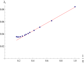
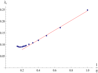
The data show that at first, as $\eta$ grows away from the initial value $\eta=1$, $\lambda_{c}$ decreases linearly with $1/\eta$, as one might expect from the relation between the $4$-dimensional ’t Hooft coupling and its $5$-dimensional counterpart, $\lambda\equiv\lambda_{5}/2\pi R$, which was used in deriving the scaling relations (52). However, at some point, $\lambda$ stops falling and seems to bottom out and start increasing or perhaps go to a constant . This is not consistent with the relation between the couplings, so it seems that the non-compact limit cannot be reached by the one-parameter scaling given by (52).

An alternative way of taking the non-compact limit is as follows. The scaling rule (52) used in the above analysis was derived from relations between $\Lambda$, $R$, $\lambda$ and $\lambda_{5}$ which follow from confinement in the underlying low-energy gauge-theory.

Figure 7: $\lambda_{c}$ as a function of $1/\eta$. These data have been obtained for $L_{\Lambda}(\eta)=L_{\Lambda}/\eta$, with $L_{\Lambda}=3/200$ and keeping $R_{\Lambda}$ fixed as $\eta$ is increased from $1$. The solid line is a power-law fit to the data.

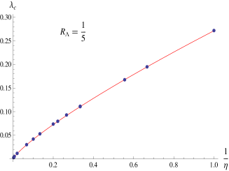
Since the non-local NJL model does not incorporate confinement, we may wish to relax these conditions among the parameters. However, we must still maintain the hierarchy of scales $L<<\pi R<<\Lambda^{-1}$. One simple way to do this is to keep $R_{\Lambda}$ fixed (and $<<1$) as $R$ is scaled. Under the scaling $R\rightarrow\eta R$, then, we must have $\Lambda\rightarrow\Lambda/\eta$. This implies that $L_{\Lambda}$ scales to $L_{\Lambda}/\eta$.

In Figure 7 we have shown data for $\lambda_{c}(\eta)$ obtained as a function of $1/\eta$ by computing the critical coupling for the set $\{R_{\Lambda},L_{\Lambda}(\eta)\}$ for different values of $\eta$. The data fit almost perfectly to a power law, $\lambda_{c}=0.271339/\eta^{0.817788}$. Since this fit implies that $\eta\lambda_{c}(\eta)$ blows up in the limit $\eta\rightarrow\infty$, the non-compact limit cannot be reached by this scaling either.

Our tentative conclusion is that possible $\chi$SB solutions in the non-compact version of the non-local NJL model cannot be obtained by taking any simple $R\rightarrow\infty$ limit of the $\chi$SB solutions of the compact model. Clearly this issue deserves to be investigated further.

6 Summary

The study of $\chi$SB in QCD is made complicated by the fact that the scale at which chiral symmetry is broken is of the order of the confinement scale. If QCD could be deformed to enable “tuning” of the $\chi$SB scale to be much smaller than the confinement scale, then one would have separated the complications of the dynamics of confinement from a study of $\chi$SB, which could then be handled by perturbative methods. The intersecting brane configuration of Sakai and Sugimoto, which gives rise to a QCD-like theory at low energies, admits just such a possibility; it has an additional parameter, the flavour brane-anti-brane separation, which can be tuned. In the strong coupling limit, by tuning this parameter one can indeed raise the chiral symmetry restoration temperature above the deconfinement temperature [21, 22]. However, as we have seen in the present work, for a consistent description of $\chi$SB in the weakly coupled SS model, it is essential to incorporate the physics of confinement. The interaction between flavour branes and anti-branes of the SS model is captured by a non-local NJL model. For any finite radius $R$ of the circle which the colour $D4$-branes wrap, there is confinement and a mass gap in the low energy theory. The NJL model reflects this dynamically generated mass scale, $\Lambda$, in the length scale over which the non-local four-fermi interaction extends. This fact turns out to be crucial in getting consistent $\chi$SB solutions. In the large $N_{c}$ limit, the question of $\chi$SB amounts to finding appropriate solutions to the non-linear gap equation. For solutions with $\chi$SB length scale $l$ much larger than the confinement scale $\Lambda^{-1}$, it is reasonable to replace the non-local NJL model by the local NJL model. Hence these solutions must reveal the existence of a critical coupling, which is known to determine $\chi$SB in the local NJL model. In this paper we have numerically solved the non-linear gap equation and verified the existence of a critical coupling below which chiral symmetry is unbroken. Roughly speaking, only solutions with $\chi$SB scale greater than the brane-anti-brane separation $L$ exist. The $\chi$SB scale $l$ increases as the ’t Hooft coupling is decreased, until a critical coupling is reached for $l\sim\Lambda^{-1}$. Solutions with $l>\Lambda^{-1}$do not lead to any further decrease in the coupling.

Our analysis is valid for any finite value of the radius $R$, which may be large. We have briefly addressed the question of what happens when $R\rightarrow\infty$. Two different ways of taking this limit, each one obtained from a well-motivated one-parameter scaling of the parameters of the SS model, were discussed. We found from our numerical data that neither of them leads to a sensible limit. The tentative conclusion is that simple ways of implementing this limit do not lead to a consistent picture of $\chi$SB in the non-compact version of the non-local NJL model. This seems to reinforce the critical role that the confinement scale plays in the compact model; the infrared cut-off provided by it enables the existence of consistent solutions to the gap equation. However, more work needs to be done to clarify this issue further.

Finally, most of the calculations reported in this paper were done numerically because the gap equation is non-linear and we could not solve it analytically. It would, however, be useful to have some analytic handle on the calculations, especially in the parameter region near the critical coupling. This could be important for a better understanding of the non-compact limit. A possible hint in this respect is the fact that excellent numerical solutions were obtained using the ansatz (50), with the constant $c$ turning out to be almost exactly equal to $l/L$ in all cases.

References

- [1]
- [2] Y. Nambu and G. Jona-Lasinio, Dynamical Model Of Elementary Particles Based On An Analogy with Superconductivity. I, Phys. Rev. 122 (1961) 345.
- [3] A. Dhar and S. R. Wadia, NambuJona-Lasinio Model: An Effective Lagrangian for Quantum Chromodynamics at Intermediate Length Scales, Phys. Rev. Lett. 52 (1984) 959.
- [4] A. Dhar, R. Shankar and S. R. Wadia, NambuJona-Lasiniotype effective Lagrangian: Anomalies and nonlinear Lagrangian of low-energy large- QCD, Phys. Rev. D31 (1985) 3256.
- [5] A. Dhar, Chiral symmetry, large-N limit and effective lagrangians in strong interactions, Invited lecture delivered at the University of Delhi Workshop in Physics (Jan. 1984), TIFR report TIFR/TH/84-25. Unpublished.
- [6] T. Hatsuda and T. Kunihiro, QCD phenomenology based on a chiral effective Lagrangian, Phys. Rept. 247 (1994) 221, hep-ph/9401310.
- [7] E. Antonyan, J. A. Harvey, S. Jensen and D. Kutasov, NJL and QCD from string theory, hep-th/0604017.
- [8] E. Antonyan, J. A. Harvey and D. Kutasov, Chiral symmetry breaking from intersecting D-branes, Nucl. Phys. B784 (2007) 1, hep-th/0608177.
- [9] T. Sakai and S. Sugimoto, Low energy hadron physics in holographic QCD, Prog. Theor. Phys. 113, 843 (2005), hep-th/0412141.
- [10] E. Witten, Anti-de Sitter space, thermal phase transitions, and confinement in gauge theories, Adv. Theor. Math. Phys. 2, 505 (1998), hep-th/9803131.
- [11] A. Karch and A. Katz, Adding flavour to AdS/CFT, JHEP 0206 (2002) 043, hep-th/0205236.
- [12] J. Babington, J. Erdmenger, N. J. Evans, Z. Guralnik and I. Kirsch, Chiral symmetry breaking and pions in non-supersymmetric gauge/gravity duals, Phys. Rev. D 69 (2004) 066007, hep-th/0306018.
- [13] M. Kruczenski, D. Mateos, R. C. Myers and D. J. Winters, Towards a holographic dual of large-N(c) QCD, JHEP 0405 (2004) 041, hep-th/0311270.
- [14] T. Sakai and S. Sugimoto, More on a holographic dual of QCD, Prog. Theor. Phys. 114, 1083 (2006), hep-th/0507073.
- [15] K. Nawa, H. Suganuma and T. Kojo, Baryons in holographic QCD, Phys. Rev. D75 (2007) 086003, hep-th/0612187.
- [16] K. Nawa, H. Suganuma and T. Kojo, Brane-induced Skyrmions: Baryons in holographic QCD, Prog. Theor. Phys. Suppl. 168 (2007) 231, hep-th/0701007.
- [17] D. K. Hong, M. Rho, H. U. Yee and P. Yi, Chiral dynamics of baryons from string theory, hep-th/0701276.
- [18] H. Hata, T. Sakai and S. Sugimoto, Baryons from instantons in holographic QCD, hep-th/0701280.
- [19] O. Bergman, G. Lifschytz and M. Lippert, Holographic nuclear physics, arXiv:0708.0326.
- [20] D. Yamada, Sakai-Sugimoto model at high density, arXiv:0707.0101.
- [21] O. Aharony, J. Sonnenschein and S. Yankielowicz, A holographic model of deconfinement and chiral symmetry restoration, Annals Phys. 322 (2007) 1420, hep-th/0604161.
- [22] A. Parnachev and D. A. Sahakyan, Chiral phase transition from string theory, Phys. Rev. Lett. 97 (2006) 111601, hep-th/0604173.
- [23] R. Casero, E. Kiritsis and A. Paredes, Chiral symmetry breaking as open string tachyon condensation, Nucl. Phys. B787 (2007) 98, hep-th/0702155.
- [24] O. Bergmann, S. Seki and J. Sonnenschein, Quark mass and condensate in HQCD, JHEP 0712 (2007) 037, arXiv:0708.2839.
- [25] A. Dhar and P. Nag, Sakai-Sugimoto model, Tachyon Condensation and Chiral symmetry Breaking, JHEP 0801 (2008) 055, arXiv:0708.3233.
- [26] A. Dhar and P. Nag, Tachyon Condensation and Quark Mass in Modified Sakai-Sugimoto Model, Phys. Rev. D78 (2008) 066021, arXiv:0804.4807.
- [27] O. Aharony and D. Kutasov, Holographic Duals of Long Open Strings, arXiv:0803.3547.
- [28] K. Hashimoto, T. Hirayama, F. Lin and H. Yee, Quark Mass Deformation of Holographic Massless QCD, arXiv:0803.4192.
- [29] K. Hashimoto, T. Sakai and S. Sugimoto, Holographic Baryons: Static Properties and Form Factors from Gauge/String Duality, Prog. Theor. Phys. 120 (2008) 1093, arXiv:0806.3122.
- [30] M. Edalati, R. G. Leigh and N. Nguyen, Transversely-intersecting D-branes at finite temperature and chiral phase transition, arXiv:0803.1277.
- [31] R. McNees, R. C. Myers and A. Sinha, On quark masses in holographic QCD, JHEP 0811 (2008) 056, arXiv:0807.5127.
- [32] P. C. Argyres, M. Edalati, R. G. Leigh and J. F. Vazquez-Poritz, Open Wilson Lines and Chiral Condensates in Thermal Holographic QCD, arXiv:0811.4617.
- [33] D. Bak and H. U. Yee, Separation of spontaneous chiral symmetry breaking and confinement via AdS/CFT correspondence, Phys. Rev. D71 (2005) 046003, hep-th/0412170.
- [34] M. E. Peskin and D. V. Schroeder, An Introduction to quantum field theory, Addison-Wesley (1995).
- [35] I. S. Gradshteyn and I. M. Ryzhik, Table of Integrals, Series, and Products, Fifth Edition, Ed. A. Jeffrey, Academic Press (1993).