Estimating the parameters of non-spinning binary black holes using ground-based gravitational-wave detectors: Statistical errors

Abstract

We assess the statistical errors in estimating the parameters of non-spinning black-hole binaries using ground-based gravitational-wave detectors. While past assessments were based on partial information provided by only the inspiral and / or ring-down pieces of the coalescence signal, the recent progress in analytical and numerical relativity enables us to make more accurate projections using “complete” inspiral-merger-ringdown waveforms. We employ the Fisher information-matrix formalism to estimate how accurately the source parameters will be measurable using a single interferometric detector as well as a network of interferometers. Those estimates are further vetted by full-fledged Monte-Carlo simulations. We find that the parameter accuracies of the complete waveform are, in general, significantly better than those of just the inspiral waveform in the case of binaries with total mass $M\gtrsim 20M_{\odot}$. In particular, for the case of the Advanced LIGO detector, parameter estimation is the most accurate in the $M=100-200M_{\odot}$ range. For an $M=100M_{\odot}$ system, the errors in measuring the total mass and the symmetric mass-ratio are reduced by an order of magnitude or more compared to inspiral waveforms. Furthermore, for binaries located at a fixed luminosity distance $d_{L}$, and observed with the Advanced LIGO–Advanced Virgo network, the sky-position error is expected to vary widely across the sky: For $M=100M_{\odot}$ systems at $d_{L}=1$Gpc, this variation ranges mostly from about a hundredth of a square-degree to about a square-degree, with an average value of nearly a tenth of a square-degree. This is more than forty times better than the average sky-position accuracy of inspiral waveforms at this mass-range. For the mass parameters as well as the sky-position, this improvement in accuracy is due partly to the increased signal-to-noise ratio and partly to the information about these parameters harnessed through the post-inspiral phases of the waveform. The error in estimating $d_{L}$ is dominated by the error in measuring the wave’s polarization and is roughly $43\%$ for low-mass ($M\sim 20M_{\odot}$) binaries and about $23\%$ for high-mass ($M\sim 100M_{\odot}$) binaries located at $d_{L}=1$Gpc.

I Introduction

Astrophysical black holes (BHs) are typically classified into three groups: stellar-mass BHs (with a mass of approximately 3 — $30M_{\odot}$), [super]massive BHs ($\sim 10^{4}$ — $10^{10}M_{\odot}$) and intermediate-mass (IM) BHs ($\sim 30$ — $10^{4}M_{\odot}$). There is strong observational evidence for the existence of both stellar-mass and supermassive BHs. The existence of stellar-mass BHs, which are the end products of stellar evolution, has been primarily inferred from observations of X-ray binaries that allow us to estimate the mass of the compact object through measurements of the orbital period and the maximum line-of-sight Doppler velocity of the companion star Narayan (2005). The mechanism for producing supermassive BHs is less certain but the acceleration of gas disks in the bulges of nearly all local massive galaxies point to their existence there Kormendy and Richstone (1995). Even more convincingly, the observations of stellar proper motion in the center of the Milky Way have confirmed the presence of a supermassive BH Schodel et al. (2002). On the other hand, the observational evidence for IMBHs is only suggestive. The main hint comes from the observations of ultraluminous X-ray sources, combined with the fact that several globular clusters show evidence for an excess of dark matter in their cores Miller and Colbert (2004).

According to hierarchical galaxy-merger models, [super]massive BH binaries should form frequently, and should be common in the cores of galaxies. There is at least one piece of clear evidence for the existence of a supermassive BH binary, namely, the X-ray active binary black hole (BBH) at the center of the galaxy NGC 6240, which is expected to coalesce in Hubble time Komossa et al. (2003). There is also growing observational evidence for the existence of many other [super]massive BBHs Ballo et al. (2004); Guainazzi et al. (2005); Evans et al. (2007); Bianchi et al. (2008). Despite the lack of any observational evidence for stellar-mass/intermediate-mass BH binaries, different mechanisms to form these binaries have been proposed in the literature (see, for e.g., Postnov and Yungelson (2006); Amaro-Seoane and Freitag (2006); Fregeau et al. (2006); Mandel et al. (2007)).

Coalescing BH binaries are among the most promising sources of gravitational waves (GWs) for the ground-based interferometric detectors. What makes them extremely interesting is that their gravitational waveforms can be accurately modelled and well parametrized by combining a variety of analytical and numerical approaches to General Relativity. To wit, the gravitational waveforms from the inspiral stage of the binary can be accurately computed by the post-Newtonian (PN) approximation to General Relativity, while those from the ring down stage can be computed using BH perturbation theory. The recent breakthrough Pretorius (2005); Campanelli et al. (2006); Baker et al. (2006) in numerical relativity has made it possible to compute accurate gravitational waveforms from the hitherto unknown merger stage as well Pretorius (2005); Campanelli et al. (2006); Baker et al. (2006); Herrmann et al. (2007); Sperhake (2006); Brügmann et al. (2006); Thornburg et al. (2007); Etienne et al. (2007).

Concomitant with that breakthrough has been the notable progress in GW instrumentation. The Initial LIGO (LIGOI) Sigg (2008) detectors have completed their first science run at design sensitivity. The Virgo detector Acernese et al. (2008) ran concurrently with LIGO for part of that run. Currently, both observatories are undergoing commissioning work with the target of achieving second-generation sensitivities over the next several years, to usher us into the era of Advanced LIGO (AdvLIGO) AdL and Advanced Virgo (AdvVirgo). Also, an intermediate, enhanced stage of LIGO, called Enhanced LIGO (EnhLIGO), is expected to be operational this year.

In the absence of any observational evidence of stellar-mass/intermediate-mass BH binaries, the rate of binary coalescence events is estimated by population synthesis studies. Plausible rate estimates for stellar-mass BH coalescences detectable by LIGOI / EnhLIGO / AdvLIGO detectors range from $7\times 10^{-4}\,/\,7\times 10^{-3}\,/\,2$ per year to $2\,/\,20\,/\,4000$ per year with a likely rate estimate of around $0.01\,/\,0.1\,/\,30$ per year O’Shaughnessy et al. (2005). For the case of IMBH binaries, the plausible rates for LIGOI / AdvLIGO detectors are $10^{-4}\,/\,0.1$ per year Fregeau et al. (2006). Similarly, for the case of stellar-mass BHs merging with IMBHs (the so-called intermediate-mass-ratio inspirals), plausible event rates for LIGOI / AdvLIGO are $10^{-3}\,/\,10$ per year Mandel et al. (2007) . A network of interferometric detectors involving LIGO, Virgo, and perhaps others, such as GEO600 Grote (2008), and TAMA Takahashi et al. (2008), will be able to extract a host of physical parameters of those sources, complementing other detectors probing their electromagnetic characteristics.

Indeed, some of the BBH mergers, e.g., triggered by the mergers of galaxies/stellar clusters harboring supermassive/intermediate-mass BHs, are likely to have electromagnetic (EM) counterparts. To associate an EM event with a GW signal from such a merger, and vice versa, one needs to be able to locate the GW source with a high enough accuracy so that the number of star clusters or galaxies in the sky-position error box is sufficiently small. As argued in Ref. Holz and Hughes (2005a), even arc-minute resolution can make such associations quite feasible. Whereas the GW observations are expected to provide more accurate distance measurements than their EM counterpart, the latter will locate the sources in the sky with far greater resolution than the former. This complementarity was explored in Ref. Schutz (1986) to argue that by combining GW and electromagnetic observations it should be possible to constrain the values of certain cosmological parameters. In particular, using the distance-redshift relation from many BBH “standard sirens”, such multi-messenger observations can put interesting constraints on the equation of state of the dark energy Holz and Hughes (2005b); Arun et al. (2007). Supermassive BH binaries are also excellent test beds for “strong-field” predictions of General Relativity (see, e.g., Arun et al. (2006a, b)). Also, GW observations of BBH coalescences can be used to test theoretical predictions such as the “no-hair” theorem Ryan (1995). The effectiveness of these and other applications depends on the accuracy with which we can estimate the parameters of the binary, which includes the component masses, distance, orientation, and sky location.

In this work, we study the effect of detector noise in limiting the accuracy with which parameters of a BBH system can be determined with the present and planned earth-based laser interferometers. In the past, in the absence of complete coalescence waveforms arising from numerical relativity, parameter estimation studies were constrained to address this question only for the inspiral/ring-down pieces of the signal present in the band of a detector Markovic (1993); Cutler and Flanagan (1994); Balasubramanian et al. (1995, 1996); Balasubramanian and Dhurandhar (1998); Nicholson and Vecchio (1998); Jaranowski et al. (1996); Poisson and Will (1995); Arun et al. (2005); Luna and Sintes (2006). Here we extend those studies to estimate how the astrophysical quest for characterizing such systems benefits from the knowledge of the complete coherent signal, comprising some or all of the inspiral, merger, and ringdown pieces, that lies in a detector’s observational band. Improvements in the accuracy of BBH parameter measurements might be expected owing to the increased signal-to-noise ratio (SNR) arising from the inclusion of the post-inspiral pieces. A second avenue toward parameter accuracy improvements can also arise, for some parameters, from the breaking of some parameter degeneracies that the extra information carried by the GW phasing of those pieces might offer. We employ the phenomenological inspiral-merger-ringdown waveforms proposed in Refs. Ajith et al. (2008a, 2007); Ajith (2008) to explore these possibilities.  The systematic errors that might arise in observations using these “complete”  BBH coalescence templates are studied in Ref. Ajith et al. (2008b).

To estimate the parameter errors, we adopt a two-pronged approach. One of these is of obtaining the Fisher information matrix and then inverting it to derive the parameter error variance-covariance matrix Helstrom (1995). The elements of this matrix are then used to obtain the lower bound on the parameter estimator errors Cramer (1946); Rao (1945). This approach is employed here, in spite of its known limitations Balasubramanian et al. (1995, 1996); Vallisneri (2008), since it has been studied extensively in the community and allows for a fair comparison of our results with those given in the literature. However, since by its very design, this bound may not be respected for signals with a low SNR (as first demonstrated by Refs. Balasubramanian et al. (1995, 1996)), we also assess estimator errors through Monte Carlo studies. For the parameter ranges considered here, the latter approach corroborates the findings of the former, with a few notable exceptions arising from parameter space boundaries, where the Monte Carlo estimates reflect better the results expected from real-data searches.

In addition to addressing the primary question on how large the parameter errors are, we also study their behavior across the BBH parameter space. We study how the various estimator errors scale with the mass parameters themselves. How much improvement do the complete waveforms impart to the determination of the sky-position of BBHs in multi-detector searches? How does the sky-position accuracy change with the BBH mass parameters? A summary of our results is as follows: First, we find that the parameter-estimation accuracies using the complete waveforms are, in general, significantly better than those using only their inspiral phases in the case of BBHs with a total mass $M\equiv(m_{1}+m_{2})\gtrsim 20M_{\odot}$, where $m_{1,2}$ are the component masses, at least for mass-ratios between 0.25 and unity. The observed trend suggests that this improvement can be expected for somewhat lower mass-ratios as well. Second, for BBHs at a fixed effective distance and $M\gtrsim 10M_{\odot}$ whereas the fractional errors in the two mass parameters, $M$ and $\eta\equiv m_{1}m_{2}/M^{2}$, scale mostly monotonically with $M$ for the inspiral-only waveforms, they do not display that property for the complete waveforms. In the latter case, they instead exhibit a distinct minimum, whose location is determined by $M$, $\eta$, and the detector’s noise power spectral-density (PSD). Third, owing to the use of complete vis à vis inspiral-only waveforms the sky-position accuracy improves by factors of many. We also show that for the complete waveforms alone, the sky-position accuracy mostly degrades with increasing total-mass when the SNR is kept fixed. This is primarily caused by a similar degradation in the estimation accuracy of the signal’s times of arrival at the different detectors in a network. This deterioration in accuracy, while not monotonic in $M$ at finer scales, is broadly so at large scales, and is caused by the reduction in the number of in-band wave cycles.

More specifically, for Advanced LIGO, the estimation of the total mass, the symmetric mass-ratio, and the effective distance $d_{\rm eff}$ is the most accurate in the $M=100-200M_{\odot}$ range. (For other detectors, that mass range is somewhat different since it is partly determined by their noise PSDs.) For such systems, the reduction of errors in parameter estimates is by an order-of-magnitude or more due to the inclusion of the post-inspiral phases. The improvement is mainly due to the expected increase in SNR arising from the inclusion of those phases. This expectation, which is based on the assumed Gaussianity and stationarity of detector noise, must be tempered by the observation that the amount of increase in SNR can be less in real data.

We also observe that for a fixed SNR, the inclusion of the post-inspiral phases improves the accuracy of $M$ and $\eta$ for a wide range of masses much more (by several times) than that of the chirp mass $M_{c}$. This is due to the fact that the inclusion of those phases helps in breaking the degeneracy between those two parameters ($M$ and $\eta$) known to exist in the inspiral waveform.

For a fixed SNR, the estimation of the luminosity distance for low-mass systems shows negligible change by the inclusion of the post-inspiral phases. This is due to its strong covariance with the polarization and the orbital inclination angles of the binary, which is mostly unaltered by the inclusion of the post-inspiral phases. Also, for a fixed SNR, the luminosity distance estimate deteriorates with increasing $M$, for reasons discussed below. On the other hand, for a fixed luminosity distance, the error in its estimate initially improves with increasing $M$, due to the increase in SNR, before degrading eventually owing to the decreasing number of in-band wave cycles.

Before moving on, we wish to point out some limitations of the present work. First, this study considers only the dominant harmonic of non-spinning BBH waveforms. Astrophysical BHs are expected to have spin, and including spin effects can change the estimation of different BBH parameters Berti et al. (2005). Whereas on the one hand previous calculations have shown that the parameter-estimation accuracies generally deteriorate upon the inclusion of spin-orbit and spin-spin couplings Berti et al. (2005); Cutler and Flanagan (1994), on the other hand the inclusion of spin-induced precession in the waveform model can improve the parameter estimation Vecchio (2004); Lang and Hughes (2006). Also, it has been noted in various studies that including the higher harmonics can significantly increase the parameter-estimation accuracies Moore and Hellings (2002); Sintes and Vecchio (1999); Van Den Broeck and Sengupta (2007); Arun et al. (2007); Trias and Sintes (2008); Porter and Cornish (2008). So, while the results presented in this paper may not be too far from the realistic case, we stress that a rigorous statement on the parameter-estimation accuracies should consider these effects as well. Moreover, neglecting spins and higher harmonics in the waveform models can result in significant amount of systematic errors in estimating various parameters. These systematic errors are out of the scope of this paper. A preliminary investigation of this is presented in Ref. Ajith et al. (2008b).

This paper is organized as follows: Sec. II briefly introduces the main aspects of the search for binary black holes. In particular, Sec. II.1 reviews the phenomenological inspiral-merger-ring down waveform templates proposed in Refs. Ajith et al. (2008a, 2007); Ajith (2008), while Sec. II.2 provides a brief introduction towards the statistical theory of parameter estimation. In Sec. III, we present the results of our calculations in the case of a search using a single interferometric detector. This section discusses the results from the analytical calculations using the Fisher-matrix formalism as well as the numerical Monte-Carlo simulations. Results from the calculations in the case of a network of detectors are discussed in Sec. IV, while Sec. V summarizes the main results and provides a discussion of the possible astrophysical implications of this work.

II Gravitational wave observations of non-spinning binary black holes

In General Relativity, the gravitational-wave strain at any point in space can be expanded in terms of its two linear polarization components $h_{+}(t)$ and $h_{\times}(t)$ or the two related circular polarization components,

$$\mathfrak{h}(t)\equiv h_{+}(t)-\mathrm{i}h_{\times}(t)=A(t)\,e^{\mathrm{i}\varphi(t)}$$ (1)

and its complex conjugate, with $\varphi(t)$ and $A(t)$ denoting the wave’s phase and amplitude. Generally, the GW emitted by a coalescing binary has multiple harmonics. In this work, we limit our study to only the dominant harmonic’s contributions to $\varphi(t)$ and $A(t)$. Then the GW strain $h(t)$ in a detector is the linear combination of the two polarization components, $h(t)=F_{+}h_{+}(t)+F_{\times}h_{\times}(t)$, with the detector’s antenna-pattern functions given as:

$$F_{+}(\theta,\phi,\psi) = -\frac{1}{2}(1+\cos^{2}\theta)\cos 2\phi~{}\cos 2\psi$$

$$- \cos\theta~{}\sin 2\phi~{}\sin 2\psi,$$

$$F_{\times}(\theta,\phi,\psi) = \frac{1}{2}(1+\cos^{2}\theta)\cos 2\phi~{}\sin 2\psi$$ (2)

$$- \cos\theta~{}\sin 2\phi~{}\cos 2\psi.$$

Above, $\theta$ and $\phi$ are the polar and azimuthal angles specifying the location of the source in the sky in the detector frame and $\psi$ is the polarization angle.

The two polarization components of the BBH signals are sinusoids with varying amplitude and frequency, and have phases $\pi/2$ radians apart relative to each other. Consequently, their GW signal in a detector can be written as:

$$h(t)=C\,A(t)\,\cos[\varphi(t)+\varphi_{0}],$$ (3)

where the amplitude coefficient $C$ and phase $\varphi_{0}$ can be assumed to be constant for signals lasting for a duration (up to several minutes) much shorter than Earth’s rotational time-scale:

$$C = \frac{1}{2}\sqrt{(1+\cos^{2}\iota)^{2}F_{+}^{2}+4\cos^{2}\iota F_{\times}^{2}},$$

$$\varphi_{0} = \tan^{-1}\left[\frac{2F_{\times}\cos\iota}{F_{+}(1+\cos^{2}\iota)}\right]\,.$$ (4)

Above, $\iota$ is angle of inclination of the orbit to the line of sight.

Figure 1: Noise amplitude spectrum ($\sqrt{S_{h}(f)}$) of different detectors considered in this paper.

II.1 Detecting non-spinning binary black holes

The GW signal’s phase $\varphi(t)$ and amplitude $A(t)$ are functions of the physical parameters of the binary, such as the component masses and the spins. Detecting a signal requires analyzing interferometric data, which are noisy. Defining a search strategy, therefore, necessitates the modelling of this noise, which we take here to be zero-mean Gaussian and stationary:

$${\overline{n(t)}} = 0,$$ (5)

$${\overline{{\tilde{n}}^{*}(f){\tilde{n}}(f^{\prime})}} = \frac{1}{2}S_{h}(f)\,\delta(f-f^{\prime})\ ,$$ (6)

with the over-bar denoting the ensemble average and the tilde denoting the Fourier transform,

$${\tilde{n}}(f)=\int_{-\infty}^{\infty}n(t)\,e^{-2\pi\mathrm{i}ft}\,{\mathrm{d}t}\,.$$ (7)

Above, $S_{h}(f)$ is the Fourier transform of the auto-covariance of the detector noise and is termed as its (one-sided) power spectral-density. We also assume the noise to be additive. This implies that when a signal is present in the data $x(t)$, then

$$x(t)=h(t)+n(t)\,.$$ (8)

The noise covariance Eq. (6) introduces the following inner-product in the function space of signals:

$$\langle a,\>b\rangle=4\Re\int_{0}^{\infty}\!{\mathrm{d}f}\>{\tilde{a}^{*}(f)\,\tilde{b}(f)\over S_{h}(f)}\ \ ,$$ (9)

where $\tilde{a}(f)$ and $\tilde{b}(f)$ are the Fourier transforms of $a(t)$ and $b(t)$, respectively.

Under the above assumptions about the characteristics of detector noise, the Neyman-Pearson criterion Helstrom (1995) leads to an optimal search statistic, which when maximized over the amplitude coefficient $C$, is the cross-correlation of the data with a normalized template,

$$\rho\equiv\langle\hat{h},x\rangle\ \ ,$$ (10)

where the normalized template is $\hat{\tilde{h}}(f)\equiv{\tilde{h}}(f)/\sqrt{\langle h,\>h\rangle}$. In a “blind” search in detector data, where none of the binary’s parameters are known a priori, the search for a GW signal requires maximizing $\rho$ over a “bank” of templates (see, for e.g., Cokelaer (2007)) corresponding to different values of those physical parameters. Apart from the physical parameters, the waveform also depends on the (unknown) initial phase $\varphi_{0}$ and the time of arrival $t_{0}$. Maximization over the initial phase $\varphi_{0}$ is effected by using two orthogonal templates for each combination of the physical parameters Schutz (1991), and the maximization over $t_{0}$ is attained efficiently with the help of the Fast Fourier Transform (FFT) algorithms Press et al. (2007).

Since the cross correlation between the data and the template can be most efficiently computed in the Fourier domain by using the FFT, waveform templates in the Fourier domain are computationally cheaper. Reference Ajith et al. (2008a) proposed a family of analytical Fourier domain templates for BBH waveforms of the form:

$${\tilde{h}}(f)\equiv{A}_{\rm eff}(f)\,e^{\mathrm{i}\Psi_{\rm eff}(f)},$$ (11)

where the effective amplitude and phase are expressed as:

$${A_{\rm eff}}(f) \equiv \frac{M^{5/6}}{d_{\rm eff}\,\pi^{2/3}}\sqrt{\frac{5\,\eta}{24}}\,f_{\rm merg}^{-7/6}\left\{\begin{array}[]{ll}\left(f/f_{\rm merg}\right)^{-7/6}&\textrm{if $f<f_{\rm merg}$}\\ \left(f/f_{\rm merg}\right)^{-2/3}&\textrm{if $f_{\rm merg}\leq f<f_{\rm ring}$}\\ w\,{\cal L}(f,f_{\rm ring},\sigma)&\textrm{if $f_{\rm ring}\leq f<f_{\rm cut}$,}\\ \end{array}\right.$$ (15)

$$\Psi_{\rm eff}(f) \equiv 2\pi ft_{0}+\varphi_{0}+\frac{1}{\eta}\,\sum_{k=0}^{7}(x_{k}\,\eta^{2}+y_{k}\,\eta+z_{k})\,(\pi Mf)^{(k-5)/3}\,.$$ (16)

In the above expressions,

$${\cal L}(f,f_{\rm ring},\sigma)\equiv\left(\frac{1}{2\pi}\right)\frac{\sigma}{(f-f_{\rm ring})^{2}+\sigma^{2}/4}\,$$ (17)

is a Lorentzian function that has a width $\sigma$, and that is centered around the frequency $f_{\rm ring}$. The normalization constant, $w\equiv\frac{\pi\sigma}{2}\left(\frac{f_{\rm ring}}{f_{\rm merg}}\right)^{-2/3}$, is chosen so as to make ${A}_{\rm eff}(f)$ continuous across the “transition” frequency $f_{\rm ring}$. The parameter $f_{\rm merg}$ is the frequency at which the power-law changes from $f^{-7/6}$ to $f^{-2/3}$. The effective distance to the binary is denoted by $d_{\rm eff}$, which is related to the luminosity distance $d_{L}$ by $d_{\rm eff}=d_{L}/C$. The phenomenological parameters $f_{\rm merg},f_{\rm ring},\sigma$ and $f_{\rm cut}$ are given in terms of the total mass $M$ and symmetric mass-ratio $\eta$ of the binary as

$$\pi Mf_{\rm merg} = a_{0}\,\eta^{2}+b_{0}\,\eta+c_{0}\,,$$

$$\pi Mf_{\rm ring} = a_{1}\,\eta^{2}+b_{1}\,\eta+c_{1}\,,$$

$$\pi M\sigma = a_{2}\,\eta^{2}+b_{2}\,\eta+c_{2}\,,$$

$$\pi Mf_{\rm cut} = a_{3}\,\eta^{2}+b_{3}\,\eta+c_{3}.$$ (18)

The coefficients $a_{j},b_{j},c_{j},~{}j=0...3$ and $x_{k},y_{k},z_{k},~{}k=0,2,3,4,6,7$ are tabulated in Table I of Ref. Ajith (2008).

II.2 Measuring binary black hole parameters

Figure 2: Errors in estimating the total mass $M$ (top left), symmetric mass ratio $\eta$ (top middle), chirp mass $M_{c}$ (top right), time of arrival $t_{0}$ (bottom left) and effective distance $d_{\rm eff}$ (bottom right) in the case of Advanced LIGO noise spectrum, plotted against the total mass of the binary. The errors of $M,\eta,M_{c}$ and $d_{\rm eff}$ are in percentage and the errors of $t_{0}$ are in seconds. The value of the symmetric mass-ratio $\eta$ is shown in legends. The solid lines correspond to a search using complete BBH templates and the dashed lines correspond to a search using 3.5PN-accurate post-Newtonian templates in the SPA, truncated at the Schwarzschild ISCO. The binary is placed optimally oriented at an effective distance of 1 Gpc.

Figure 3: Same as in Fig. 2 except that the binary is placed at an effective distance of 100 Mpc and the noise PSD corresponds to that of Initial LIGO.

Figure 4: Same as in Fig. 2 except that the binary is placed at an effective distance of 100 Mpc and the noise PSD corresponds to that of Enhanced LIGO.

To evaluate how effective the detectors will be in establishing the field of GW astronomy, especially, with the second-generation Earth-based interferometers scheduled to come online around 2014, one needs to foremost assess how accurately they can measure the astrophysical properties of compact object binaries. That quest will be limited, on the one hand, by the accuracy with which the search templates can model actual gravitational waveforms, and, on the other hand, by the inherent statistical noise in the measurement process. The former issue is one of systematics, which will be discussed elsewhere (see, e.g., Ref. Ajith et al. (2008b)). Here, we discuss the latter issue in more detail.

To determine how large the noise-limited errors can be in the measured values of the signal parameter, we take those values to be the maximum likelihood estimators (MLEs). The discussion in the preceding section shows that a total of nine parameters characterize the non-spinning BBH coalescence signals considered here. They are the total mass $M$, the symmetric mass-ratio $\eta$, the sky-position angles $(\theta,\phi)$, the binary’s orientation angles $(\psi,\iota)$, the luminosity distance $d_{L}$, the initial (or some reference) phase $\varphi_{0}$, and the time of arrival (or some reference time) $t_{0}$. For computing the error estimates, we map them onto the components of the parameter vector, $\mbox{\boldmath$\vartheta$}\equiv\{\ln\mathcal{A},t_{0},\varphi_{0},\ln M,\ln\eta,\theta,\phi,\psi,\iota\}$, where $\mathcal{A}=\frac{M^{5/6}}{d_{\rm eff}\pi^{3/2}}\sqrt{\frac{5\eta}{24}}$. Owing to noise, their MLEs, $\hat{\mbox{\boldmath$\vartheta$}}$, will expectedly fluctuate about the true values, i.e., $\hat{\mbox{\boldmath$\vartheta$}}=\mbox{\boldmath$\vartheta$}+\delta\mbox{\boldmath$\vartheta$}$, where $\delta\mbox{$\vartheta^{a}$}$ is the random error in estimating the parameter $\vartheta^{a}$. The magnitude of these fluctuations can be quantified by the elements of the variance-covariance matrix, $\gamma^{ab}=\ \overline{\delta\vartheta^{a}\,\delta\vartheta^{b}}$ Helstrom (1995).

A relation between the $\gamma^{ab}$ and the signal is available through the Cramer-Rao inequality, which dictates that

$$\parallel{\mbox{\boldmath$\gamma$}}\parallel~{}\geq~{}\parallel{\mbox{\boldmath$\Gamma$}}\parallel^{-1}\ \ ,$$ (19)

where $\Gamma$ is the Fisher information matrix:

$$\Gamma_{ab} = \sum_{I=1}^{N}\left<\partial_{a}{\tilde{h}}^{I}(\mbox{\boldmath$\vartheta$}),\partial_{b}{\tilde{h}}^{I}(\mbox{\boldmath$\vartheta$})\right>_{(I)}$$ (20)

$$\equiv \sum_{I=1}^{N}4\Re\int{\mathrm{d}f}~{}{\partial_{a}{\tilde{h}}^{I*}(f;\mbox{\boldmath$\vartheta$})~{}\partial_{b}{h}^{I}(f;\mbox{\boldmath$\vartheta$})\over S_{h}^{I}(f)},$$

where $I$ is the detector index and $\partial_{a}$ denotes taking partial derivative with respect to the parameter $\vartheta^{a}$. Therefore, $\Delta\vartheta^{a}\equiv\left(~{}\overline{\delta\vartheta^{a}\,\delta\vartheta^{a}}~{}\right)^{1/2}=\Gamma_{aa}^{-1/2}$ gives the lower bound on the root-mean-square (rms) error in estimating $\vartheta^{a}$. The two are equal in the limit of large SNR (see, e.g., Vallisneri (2008)).

The errors in the sky-position angles will be presented in terms of the error in the measurement of the sky-position solid angle, defined as:

$$\Delta\Omega=2\pi\sqrt{(\Delta\cos\theta\,\Delta\phi)^{2}-\left(~{}\overline{\delta\cos\theta~{}\delta\phi}~{}\right)^{2}}\,.$$ (21)

Each parameter-error, $\Delta\vartheta^{a}$, falls off inversely with SNR. Since the solid angle is two dimensional, its error falls off quadratically with SNR Helstrom (1995); Cutler (1998); Rogan and Bose (2006).

III Parameter estimation: Single-detector search

Figure 5: The overlap function (i.e., the ambiguity function maximized over $t_{0}$ and $\varphi_{0}$) between waveforms constructed at different points in the parameter space. The horizontal axis reports the total mass $M$ of the binary while the vertical axis reports its symmetric mass-ratio $\eta$. Each panel shows the overlap of different waveforms with one “target waveform”. The total mass of the target waveform is chosen to be $M=20M_{\odot},~{}100M_{\odot},~{}200M_{\odot},~{}400M_{\odot}$, respectively, for the four columns starting from the left. The symmetric mass-ratio of the target waveforms is chosen to be $\eta=0.25,~{}0.222,~{}0.16$ in the top, middle and bottom rows, respectively.

Figure 6: Errors in estimating the total mass $M$ (top left), symmetric mass ratio $\eta$ (top middle), chirp mass $M_{c}$ (top right), time of arrival $t_{0}$ (bottom left) and effective distance $d_{\rm eff}$ (bottom right) in the case of Advanced LIGO noise spectrum, plotted against the total mass of the binary. The errors of $M,\eta,M_{c}$ and $d_{\rm eff}$ are in percentage and the errors of $t_{0}$ is in seconds. Symmetric mass-ratio $\eta$ is shown in legends. The solid lines correspond to a search using complete BBH templates and the dashed lines correspond to 3.5PN-accurate post-Newtonian templates in the SPA, truncated at the Schwarzschild ISCO. The errors correspond to a fixed SNR of 10.

Figure 7: Same as Fig. 6 except that the noise PSD corresponds to that of Initial LIGO.

Figure 8: Same as Fig. 6 except that the noise PSD corresponds to that of Enhanced LIGO.

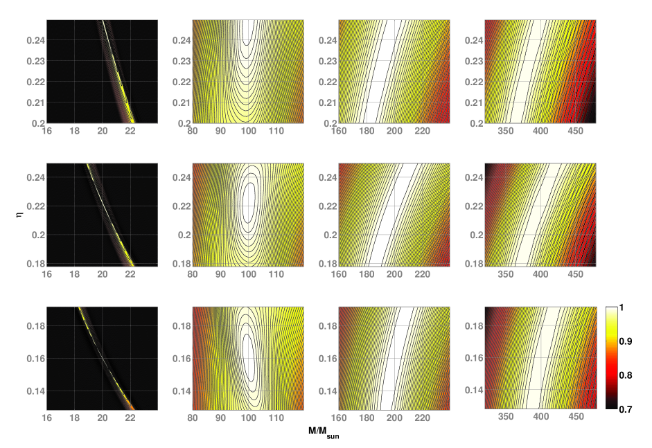
III.1 Analytical calculation using Fisher information matrix

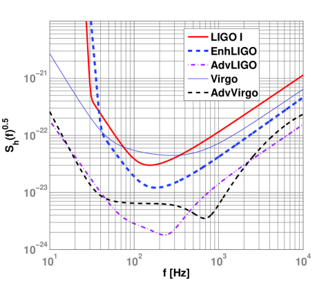
In this section, we use the Fisher information-matrix formalism to estimate the errors in measuring the parameters of coalescing BBHs with a single GW interferometer. We present results for three generations of ground-based detectors, namely, Initial LIGO, Enhanced LIGO and Advanced LIGO. The one-sided noise PSD of the Initial LIGO detector is given in terms of a dimensionless frequency $x=f/f_{0}$ by Damour et al. (2001); LAL

$$S_{h}\left(f(x)\right)=9\times 10^{-46}\left[(4.49x)^{-56}+0.16x^{-4.52}+0.52+0.32x^{2}\right]\,,$$ (22)

where $f_{0}=150$ Hz; while the same for Enhanced LIGO reads Adhikari :

$$S_{h}\left(f(x)\right)=1.5\times 10^{-46}\left[1.33\times 10^{-27}\,e^{-5.5\,(\ln\,x)^{2}}\,x^{-52.6}\,+0.16\,x^{-4.2}+0.52+0.3\,x^{2.1}\right],$$ (23)

where $f_{0}=178$ Hz. For Advanced LIGO LAL ,

$$S_{h}\left(f(x)\right)=10^{-49}\left[x^{-4.14}-5x^{-2}+111\Big{(}\frac{1-x^{2}+x^{4}/2}{1+x^{2}/2}\Big{)}\right]\,,$$ (24)

where $f_{0}=215$ Hz, and, for Advanced Virgo Losurdo ,

$$S_{h}\left(f(x)\right)=10^{-47}\left[2.67\times 10^{-7}x^{-5.6}+0.59\,e^{(\ln\,x)^{2}\,[-3.2-1.08\ln(x)-0.13(\ln\,x)^{2}]}\,x^{-4.1}+0.68\,e^{-0.73(\ln\,x)^{2}}\,x^{5.34}\right]\,,$$ (25)

where $f_{0}=720$ Hz. The calculations presented in this section were performed using the Initial LIGO, Enhanced LIGO and Advanced LIGO noise PSDs, while the calculations presented in Sec. IV consider a three-detector network consisting of Advanced LIGO and Advanced Virgo.

The parameters that can be estimated through single-detector observations are $\{\mathcal{A}(d_{L}),t_{0},\varphi_{0},M,\eta\}$. To be precise, one can measure only the Doppler-shifted masses, unless there are additional experiments for determining the Doppler-shift Cutler and Flanagan (1994) and, therefore, allow the estimation of the true masses. Doppler shifting can arise due to the motion of the detector relative to the source or the cosmological expansion. In measurements with multiple-detectors, as discussed below, it is possible to measure the source distance and sky-position as well. There too, the distance observed is actually the Doppler-shifted distance.

The Fisher matrix elements in the $\{\mathcal{A},t_{0},\varphi_{0},M,\eta\}$ space are computed from the derivatives of the waveforms described by Eqs.(11) – (18):

$$\Gamma_{ab}=\left<\partial_{a}\tilde{h}(f),\partial_{b}\tilde{h}(f)\right>\simeq 4\,\int_{f_{\rm low}}^{f_{\rm cut}}{\mathrm{d}f}~{}\frac{\partial_{a}A_{\rm eff}(f)\,\partial_{b}A_{\rm eff}(f)+A_{\rm eff}^{2}(f)\,\partial_{a}\Psi_{\rm eff}(f)\,\partial_{b}\Psi_{\rm eff}(f)}{S_{h}(f)}\,,$$ (26)

where the low-frequency cutoff, $f_{\rm low}$, is chosen to be 10 Hz for Advanced LIGO, and 40 Hz for Enhanced and Initial LIGOs. The upper-frequency cuttoff, $f_{\rm cut}$ is given by Eq. (18).

The rms errors in parameters $M,\eta$ and $t_{0}$ are computed by inverting the Fisher matrix elements as discussed in Sec. II.2. The error in estimating the chirp mass $M_{c}$ and the effective distance $d_{\rm eff}$ are obtained by propagating the errors in $M,\eta$ and $\mathcal{A}$ in the following way:

$$\left(\frac{\Delta M_{c}}{M_{c}}\right)^{2} = \left(\frac{\Delta M}{M}\right)^{2}+\frac{9}{25}\left(\frac{\Delta\eta}{\eta}\right)^{2}$$ (27)

$$+ \frac{6}{5}\,\mathcal{C}_{M\eta}\,\frac{\Delta M}{M}\,\frac{\Delta\eta}{\eta}$$

$$\left(\frac{\Delta d_{\rm eff}}{d_{\rm eff}}\right)^{2} = \frac{25}{36}\left(\frac{\Delta M}{M}\right)^{2}+\frac{1}{4}\left(\frac{\Delta\eta}{\eta}\right)^{2}+\left(\frac{\Delta\mathcal{A}}{\mathcal{A}}\right)^{2}$$ (28)

$$+ \frac{5}{6}\mathcal{C}_{M\eta}\frac{\Delta M}{M}\,\frac{\Delta\eta}{\eta}-\frac{5}{3}\mathcal{C}_{M\mathcal{A}}\frac{\Delta M}{M}\,\frac{\Delta\mathcal{A}}{\mathcal{A}}$$

$$- \mathcal{C}_{\eta\mathcal{A}}\frac{\Delta\eta}{\eta}\,\frac{\Delta\mathcal{A}}{\mathcal{A}}$$

where $\Delta\vartheta^{a}$ denotes the rms error in estimating $\vartheta^{a}$ obtained from $\Gamma_{ab}$, and $\mathcal{C}_{ab}$ is the correlation coefficient between parameters $\vartheta^{a}$ and $\vartheta^{b}$.

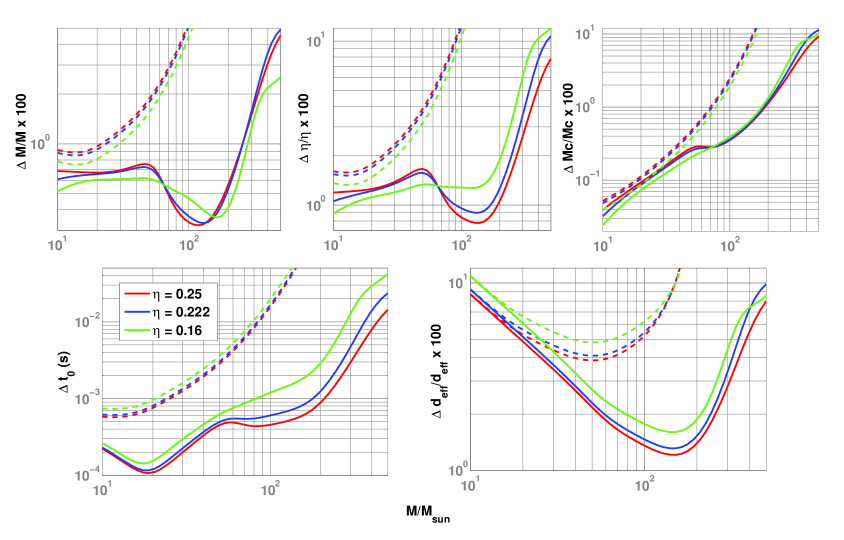
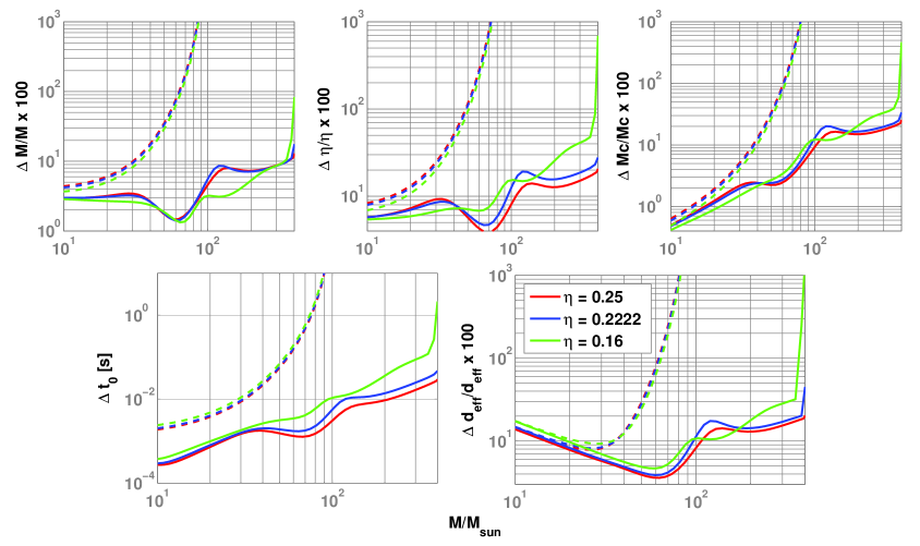
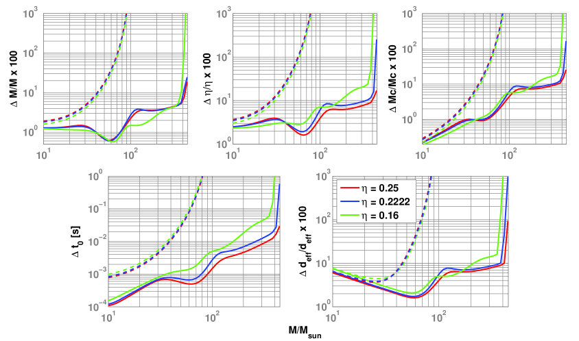
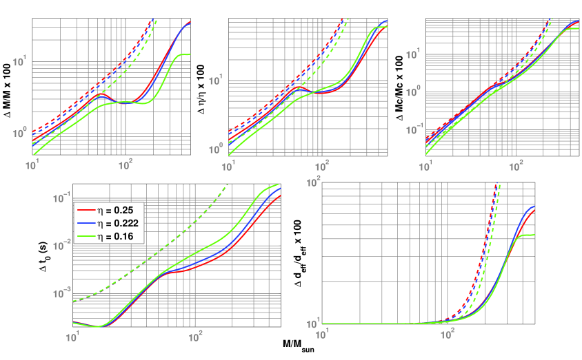
Errors in the estimates of the parameters $M,\eta,M_{c},t_{0}$ and $d_{\rm eff}$ in the case of AdvLIGO detector are plotted against the total mass $M$ in Fig. 2. These errors are computed assuming that the binary is placed at an effective distance of 1 Gpc. Also plotted in the figures are the same error-bounds computed from the 3.5PN accurate restricted PN waveforms in the stationary phase approximation (SPA), truncated at the Schwarzschild innermost stable circular orbit (ISCO). It can be seen that, over a significant range of the total mass, the error-bounds in the complete templates are largely better than those in the PN inspiral waveforms. For binaries with $M=100M_{\odot}$ and $\eta=0.25$, the error-bounds in various parameters using the complete [PN] templates are $\Delta M/M\simeq 0.34\,[5.38]\,\%,~{}\Delta\eta/\eta\simeq 0.84\,[12.98]\,\%,~{}\Delta M_{c}/M_{c}\simeq 0.35\,[2.47]\,\%,~{}\Delta t_{0}\simeq 0.46\,[15.51]$ ms and $\Delta d_{\rm eff}/d_{\rm eff}\simeq 1.36\,[5.24]\,\%$. The errors in estimating the same parameters using Initial LIGO and Enhanced LIGO detectors are plotted in Figs. 3 and 4.

The rate of variation in the errors in different regions of the parameter space can be understood by studying the overlap function, which is the ambiguity function maximized over $t_{0}$ and $\varphi_{0}$ Sathyaprakash and Dhurandhar (1991). Figure 5 plots the contours of the overlap between waveforms generated at different points in the $(M,\eta)$ space. Notice the change in the shape and orientation of the ambiguity ellipses, especially, as the total mass of the binary is varied. While, to a very good approximation, the chirp mass continues to remain as one of the eigen-coordinate Sathyaprakash (1994) in the case of the low-mass (with $M\leq 20M_{\odot})$ binary inspiral (PN) waveforms, this is no longer true for the complete waveforms of higher mass systems. This is because the latter waveforms have more information about the component masses than just the chirp mass. The eigen-directions change dramatically with increasing total mass. It can be seen that the error trends reported in Fig. 2 closely follow the shape of these ambiguity ellipses. This also means that while placing templates in the inspiral-merger-ring down searches, we will have to consider these changes in the orientation of the ambiguity ellipses. This will be studied in a future work.

One common problem encountered in the estimation of errors using Fisher information matrix is the following: In some cases (especially in the case of large number of parameters), the Fisher matrix becomes badly conditioned, thereby, decreasing the fidelity of the error covariance matrix derived by inverting it. This problem can often be obviated by intelligently choosing the parameters and by projecting out certain dimensions in the Fisher matrix (e.g., $t_{0}$ and $\varphi_{0}$). We have verified our results by comparing the errors computed using the full Fisher matrix with those computed using the projected matrix. In our calculations, they turned out to be the same to the extent discernible in the figures and tables presented here.

It may be noted that for a fiducial signal limited only to the inspiral phase of the binary, i.e., for $f<f_{\rm merg}$, the parameter $\mathcal{A}$ is uncorrelated with the other signal parameters, and hence one has $\Gamma_{1a}=\delta_{1a}\,\rho^{2}$, which renders the Fisher matrix in the block-diagonal form. However, for the complete signal, with the merger and the ringdown pieces included, the correlation of $\mathcal{A}$ with the other parameters becomes non zero, and the Fisher matrix is no longer block-diagonal with respect to this parameter. This implies that the complete waveforms provide more information about $\mathcal{A}$ and, hence, about the effective distance $d_{\rm eff}$.

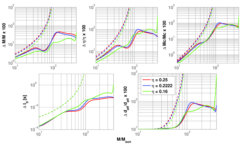
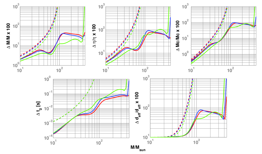
Figures 6, 7 and 8 show the error estimates corresponding to a fixed (single-detector) SNR of 10 in the case of Advanced LIGO, Initial LIGO and Enhanced LIGO noise spectra, respectively. It is interesting to note that the parameter estimation using the complete waveforms is still much better than that using only the inspiral waveform even though, in order to produce the same SNR using inspiral templates, the effective distance to the binary has to be often much smaller. The reason for this can be understood through an analogy with parameter estimation with multiple detectors: Since the inspiral phase, on the one hand, and the merger-ringdown phases, on the other hand, occupy two contiguous and, essentially, non-overlapping frequency-bands, the detection of a complete signal is equivalent to a coherent detection of these two pieces of the waveforms by two coincident, co-aligned detectors with sensitivities limited to the two contiguous bands, respectively. The two phases, however, are modulated by the two mass parameters in complementary ways, in the sense that the Fisher sub-matrices in the two-dimensional mass-space for these two fiducial detectors grow more linearly independent of each other, the larger the total mass gets, even while the total coherent SNR of this fiducial detector pair is held constant. This linear independence causes the estimation of two mass parameters to improve. Contrastingly, since the merger-ringdown pieces add very little information about a system’s chirp-mass, the improvement in its accuracy arising from using complete waveforms is much less even for high mass systems.

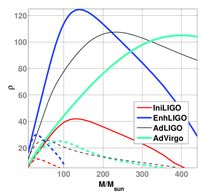
Figure 9 plots the SNR produced at different detectors by equal-mass binaries located at a fixed distance, as a function of the total mass of the binary.

Figure 9: The curves labelled “IniLIGO” and “EnhLIGO” report the SNR produced by binaries located at an effective distance of 100Mpc at Initial LIGO and Enhanced LIGO, respectively, as a function of the total mass. The curves labelled “AdLIGO” and “AdVirgo” report the same produced by binaries located at 1Gpc at Advanced LIGO and Advanced Virgo. The solid lines correspond to complete waveforms and the dashed lines correspond to PN waveforms.

III.2 Monte-Carlo simulations

Figure 10: Scatter plot of parameters estimated from $10^{4}$ Monte-Carlo simulations. The horizontal axis reports the total mass and the vertical axis reports the symmetric mass ratio. The left panel correspond to the injection with parameters $M=20M_{\odot}$ and $\eta=0.2222$, and the right panel correspond the injection with parameters $M=200M_{\odot}$ and $\eta=0.2222$. The injections correspond to an SNR of 20. Also overlaid in the left panel is a cartoon of the four different initial simplexes chosen for the maximization algorithm. The true values of the parameters is marked by a cross. Note that the eigen directions are different in the two plots.

Figure 11: Distribution of the estimated parameters from Monte-Carlo simulations and expected probability distributions from Fisher matrix calculation. The true parameters are $M=20M_{\odot},\eta=0.16$.

Figure 12: The data points show the errors computed from Monte-Carlo simulations in the case of Advanced LIGO noise PSD. The horizontal axis reports the total mass while the legends report the symmetric mass ratio. The errors are computed for a fixed SNR of 20. The dashed lines correspond to the same errors computed using Fisher matrix formalism.

	$\eta=0.25$			$\eta=0.2222$			$\eta=0.16$
$\rho$	$M=20M_{\odot}$	$100M_{\odot}$	$200M_{\odot}$	$20M_{\odot}$	$100M_{\odot}$	$200M_{\odot}$	$20M_{\odot}$	$100M_{\odot}$	$200M_{\odot}$
$\Delta M/M\times 100$
6	2.30 (1.52)	4.35 (3.80)	10.0 (5.59)	2.12 (2.15)	4.37 (4.31)	8.50 (6.58)	1.66 (1.80)	4.59 (4.58)	5.11 (5.74)
10	1.38 (0.93)	2.61 (2.39)	6.02 (3.57)	1.27 (1.50)	2.62 (2.60)	5.10 (4.49)	1.00 (1.16)	2.75 (2.58)	3.07 (3.61)
20	0.69 (0.46)	1.30 (1.11)	3.01 (1.94)	0.64 (0.76)	1.31 (1.20)	2.55 (2.73)	0.50 (0.60)	1.38 (1.21)	1.53 (1.81)
40	0.34 (0.19)	0.65 (0.51)	1.50 (0.95)	0.32 (0.34)	0.66 (0.56)	1.28 (1.33)	0.25 (0.25)	0.69 (0.61)	0.77 (0.83)
100	0.14 (0.07)	0.26 (0.18)	0.60 (0.31)	0.13 (0.11)	0.26 (0.20)	0.51 (0.46)	0.10 (0.08)	0.28 (0.24)	0.31 (0.28)
$\Delta\eta/\eta\times 100$
6	4.30 (2.51)	10.9 (4.40)	18.8 (6.93)	3.94 (3.98)	11.5 (7.25)	20.2 (10.2)	3.06 (3.29)	12.5 (9.98)	23.6 (15.4)
10	2.58 (1.77)	6.54 (3.13)	11.3 (4.96)	2.36 (2.96)	6.87 (5.26)	12.1 (9.58)	1.84 (2.27)	7.53 (6.64)	14.2 (12.1)
20	1.29 (0.88)	3.27 (1.54)	5.64 (2.93)	1.18 (1.45)	3.44 (3.01)	6.06 (6.43)	0.92 (1.13)	3.76 (3.44)	7.07 (7.25)
40	0.64 (0.36)	1.63 (0.69)	2.82 (1.48)	0.59 (0.65)	1.72 (1.45)	3.03 (3.25)	0.46 (0.47)	1.88 (1.69)	3.54 (3.63)
100	0.26 (0.14)	0.65 (0.29)	1.13 (0.52)	0.24 (0.21)	0.69 (0.53)	1.21 (1.16)	0.18 (0.15)	0.75 (0.67)	1.41 (1.33)
$\Delta M_{c}/M_{c}\times 100$
6	0.32 (0.94)	4.56 (3.86)	19.8 (7.92)	0.28 (1.16)	4.34 (4.64)	19.0 (10.6)	0.20 (1.16)	3.85 (4.22)	16.5 (12.0)
10	0.19 (0.31)	2.73 (2.62)	11.9 (5.56)	0.17 (0.35)	2.60 (3.20)	11.4 (9.30)	0.12 (0.26)	2.31 (2.76)	9.92 (9.51)
20	0.10 (0.10)	1.37 (1.24)	5.95 (3.23)	0.08 (0.13)	1.30 (1.65)	5.70 (6.24)	0.06 (0.09)	1.15 (1.45)	4.96 (5.52)
40	0.05 (0.03)	0.68 (0.55)	2.97 (1.64)	0.04 (0.05)	0.65 (0.68)	2.85 (3.14)	0.03 (0.03)	0.58 (0.59)	2.48 (2.67)
100	0.02 (0.01)	0.27 (0.20)	1.19 (0.57)	0.02 (0.01)	0.26 (0.26)	1.14 (1.11)	0.01 (0.01)	0.23 (0.23)	0.99 (0.97)
$\Delta d_{\rm eff}/d_{\rm eff}\times 100$
6	16.7	17.6	24.6	16.7	17.5	24.3	16.7	17.4	23.2
10	10.0	10.5	14.8	10.0	10.5	14.6	10.0	10.4	13.9
20	5.00	5.27	7.39	5.00	5.26	7.30	5.00	5.21	6.95
40	2.50	2.63	3.70	2.50	2.63	3.65	2.50	2.61	3.48
100	1.00	1.05	1.48	1.00	1.05	1.46	1.00	1.04	1.39
$\Delta t_{0}({\rm ms})$
6	0.37	5.90	15.8	0.39	7.22	20.0	0.42	11.7	36.3
10	0.22	3.54	9.47	0.23	4.33	12.0	0.25	7.04	21.8
20	0.11	1.77	4.73	0.12	2.17	6.00	0.13	3.52	10.9
40	0.06	0.88	2.37	0.06	1.08	3.00	0.06	1.76	5.45
100	0.02	0.35	0.95	0.02	0.43	1.20	0.03	0.70	2.18

Table 1: Errors in estimating different prameters of the binary, as a function of the binary parameters and the SNR, computed using the Fisher matrix formalism. Same errors computed from the Monte-Carlo simulations are shown in brackets.

Figure 13: Errors computed from Monte-Carlo simulations (crosses, dots and diamonds) plotted against SNR. The horizontal axes report the SNR of the injections and the legends report the total mass in units of $M_{\odot}$. The top, middle and bottom panels correspond to mass ratios $\eta=0.25,0.2222$ and $0.16$, respectively. The error-bounds expected from the Fisher matrix calculation are indicated by dashed lines.

The limitations of the Fisher-matrix formalism are well known Balasubramanian et al. (1995, 1996); Vallisneri (2008). The parameter-error bounds provided by it are trustworthy in the limit of high SNR and for parameters on which the signal has linear dependence. In the case of low SNRs the error bounds computed using the Fisher matrix formalism can be largely different from the “actual” errors. Also, the Fisher matrix does not recognize the boundaries of the parameter space (such as the restriction $\eta\leq 0.25$). Neither does it account for practical restrictions such as the finite sampling of the data. In order to explore these limits of the Fisher formalism, we performed Monte-Carlo simulations, whereby maximum-likelihood detections were made of simulated signals added to multiple statistically independent realizations of simulated colored, Gaussian noise. The aim of this frequentist study was to obtain the spread in the maximum-likelihood estimates of the parameters and compare them with Fisher-matrix calculations. It is worth clarifying that there is another interesting question one can pose in the context of parameter estimation, namely, “Given a specific signal and a particular noise realization, what are the posterior distributions of the parameter estimates.” This is a question from Bayesian statistics that can be answered using Markov-Chain Monte-Carlo (MCMC) simulations, as explored for inspiral-only waveforms in Refs. Röver et al. (2006); van der Sluys et al. (2007); Raymond et al. (2008); van der Sluys et al. (2008). We do not answer that question here.

In this section we present results from the frequentist Monte-Carlo simulation studies. These studies largely corroborate the Fisher matrix calculations in the parameter-space regions where the latter is expected to be trustworthy. The simulations also allow us to compute error-bounds in the parameter-space regions where the Fisher matrix formalism can be unreliable (such as for $\eta\simeq 0.25$). We caution the reader that this is not meant to be an exhaustive comparison between Fisher-matrix calculations and Monte-Carlo simulations. A detailed comparison of Fisher matrix formalism with Monte-Carlo simulations in the case of 3.5PN inspiral signals can be found in the recent work Ref. Cokelaer (2008).

Colored Gaussian noise with one-sided PSD $S_{h}(f)$ is generated in the frequency domain. If $\hat{x}_{k}$ and $\hat{y}_{k}$ denote the real and imaginary parts of the discrete Fourier transform of the noise at the frequency bin $k$, these are generated by

$$\hat{x}_{k}=\sqrt{S_{h_{k}}}\,x_{k}/2~{},~{}~{}~{}\hat{y}_{k}=\sqrt{S_{h_{k}}}\,y_{k}/2,$$ (29)

where $x_{k}$ and $y_{k}$ are random variables drawn from a Gaussian distribution of zero mean and unit variance, and $S_{h_{k}}$ denotes the discrete version of $S_{h}(f)$. Frequency domain signal described by Eq.(11) is added to the noise. The data is filtered through a matched filter employing templates described by Eq.(11). The likelihood is maximized over $t_{0}$ and $\varphi_{0}$ as described in Sec. II. The maximization over the physical parameters ($M$ and $\eta$) is best performed by filtering the data using a template bank finely spaced in the parameter space. But, in order to attain sufficiently good accuracy (say, $1\%$), a large number of simulations needs to be performed. Thus, computing error-bounds from a good volume of the parameter space is computationally expensive in a template bank search. So, in this paper, the maximization over the physical parameters is performed with the aid of the computationally cheaper Nelder-Mead downhill simplex algorithm Nelder and Mead (1964).

We emphasize that this search may not be as accurate as the template bank search. One reason for the inaccuracy is that, in this method, we do not “sample” the parameter space finely enough, and hence the “real maximum” can very well be missed. This is especially the case when the function that we want to maximise (likelihood in this case) contains many secondary maxima. Indeed, it is well known that the the likelihood can have many secondary maxima arising due to global correlations in the parameter space. We bypass this issue by starting the maximisation algorithm around the “actual” peak of the function. Hence, the error distributions that we obtain are only indicative of the spread of the MLM estimates around the primary maxima. Unlike in the case of MCMC simulations, this does not provide a complete picture of the posterior distribution of the parameters. Nevertheless, this is a worthwhile tool as an independent verification of the Fisher matrix calculation, enabling us to “scan”’ a good volume of the parameter space using Monte-Carlo simulations .

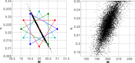
Nelder-Mead’s algorithm is a multidimensional minimisation/maximisation algorithm. In order to maximize the required function, we need to specify an initial “simplex” of $n+1$ dimensions where $n$ is the dimensionality of the parameter space. Since the dimensionality of our parameter space is 2, the simplex in our case is a triangle. It is important for the good convergence of the maximization that the initial simplex “catch” the orientation of the ambiguity ellipses in our parameter space, which often depends strongly on the parameters themselves. Thus, we start the maximization by specifying four different initial simplexes, whose vertices have equal (coordinate) distance from the “true” value of the parameters. The four triangles are oriented in different directions in the parameter space. We choose the parameters corresponding to the best among the maximized likelihoods as the parameters of the injection. Figure 10 shows a scatter plot of the parameters estimated from $10^{4}$ simulations. Also overlaid in the left plot is a cartoon of the initial simplexes chosen. The reader may note the difference in the eigen-directions in the two plots.

We found that the following points need to be taken care of while performing this kind of simulations: (i) Since the frequency-domain templates are abruptly cut off at the frequency $f_{\rm cut}$, we need to make sure that the edges arising from this do not corrupt our numerical calculations. This means that, for high mass systems ($M>200M_{\odot}$) we cannot perform the simulations with very high SNR ($\rho>100$), because the cutoff frequency is at the “sweet spot” of the detector. (ii) Sufficiently small tolerance level for the maximization algorithm in order to ensure that the “true” maximum is never missed. (iii) Orthonormality of the search templates, as emphasized by Ref. Balasubramanian et al. (1996).

The frequency distributions of the estimated parameters $M,\eta$ and $M_{c}$ are shown in Fig. 11. The injection corresponds to the parameter values $M=20M_{\odot}$ and $\eta=0.16$ and an SNR of 20. Also plotted in the figures are the expected distributions computed using the Fisher matrix formalism. All the results are computed using the AdvLIGO noise PSD. It can be seen that the two calculations agree very well. Figure 12 shows the errors computed using the Monte-Carlo simulations plotted against the total mass of the binary for three different values of $\eta$. The simulations are performed with an SNR of 20. Also shown are the error-bounds computed using the Fisher matrix formalism. In the case of mass ratios $\eta=0.2222$ and $\eta=0.16$, the simulations agree well with the Fisher matrix calculations. But the simulations disagree with the Fisher calculations for the case of $\eta=0.25$. This is expected because the Fisher matrix does not recognize the physical restriction that $\eta$ can only take values less than, or equal to 0.25. The Fisher matrix calculation assumes that the errors in estimating the parameters are Gaussian distributions centered around $\eta=0.25$, while the Monte-Carlo simulations enforce the restriction $\eta\leq 0.25$. As a result the error bounds estimated by the Monte-Carlo simulations will be less than that estimated by the Fisher matrix.

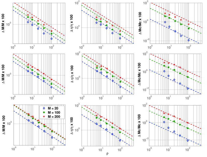
Fisher matrix calculations assume that the errors decrease inversely proportional to the SNR. But this approximation is not valid at low SNRs. So we have performed Monte-Carlo simulations with various SNRs in order to study the SNR dependence of the errors. Figure 13 plots the errors estimated from the simulations against the SNR of the injections. The top, middle and bottom panels in the figure correspond to mass ratios $\eta=0.25,0.2222$ and $0.16$, respectively. The different markers correspond to the Monte-Carlo simulations and the dashed lines correspond to the Fisher matrix calculations. It can be seen that, barring the case of $\eta=0.25$, the simulations agree very well with the Fisher calculations in the limit of high SNRs ($\rho>10$). Because of the $\eta$-boundary effects, the errors computed from the $\eta=0.25$ simulations are less than those computed from the Fisher calculations. For small SNRs ($\rho\leq 10$), the simulation errors start to deviate from the Fisher calculations. There are two reasons for this: (i) at low SNRs, as observed by many others (see, for e.g., Ref. Balasubramanian et al. (1996)) the Fisher matrix largely underestimates the errors. This is the dominating effect in the case of $M=20M_{\odot}$ binaries at low SNRs in Fig. 13. (ii) at low SNRs, since the size of the ambiguity ellipses are increased, they are cut by the $\eta=0.25$ boundary, which is neglected by the Fisher calculations. Hence the Fisher matrix over estimate the errors. This is the dominating effect in the case of $M=200M_{\odot}$ binaries at low SNRs. It is the interplay between these two competing effects that causes the discrepancy between the simulations and Fisher calculations. In summary, the results from the Monte-Carlo simulations, albeit the limitations of the maximization algorithm used, should be more reliable than the Fisher calculations.

Table 1 tabulates the errors in the case of Advanced LIGO noise PSD, computed using both Fisher matrix and Monte-Carlo simulations.

IV Parameter estimation: Multi-detector search

Figure 14: The network SNR of a signal, corresponding to the complete waveform, from an equal-mass binary with $M=100M_{\odot}$ located at $d_{L}$ = 1Gpc, plotted as a function of its sky-position. The network here is the three detector AdvLIGO-AdvVirgo network, such that the two 4km-arm-length LIGO detectors in Hanford and Livingston have AdvLIGO noise PSDs and the Virgo detector in Cascina has AdvVirgo noise PSD. Above, $\theta$ and $\phi$ are the polar and azimuthal angles specifying the location of the source in the sky in the geographic coordinate system.

Figure 15: The left plot shows the sky-position error $\log_{10}$[$\Delta\Omega$ (in square-degrees)] and the right plot shows the fractional error in the luminosity distance $\log_{10}$[$\Delta d_{L}/d_{L}$ (in %)] as functions of the sky-position of a BBH source. The source studied here is the same equal-mass binary considered in Fig. 14, and, $\theta$ and $\phi$ are the polar and azimuthal angles specifying the location of the source in the sky in the geographic coordinate system. Note how the effect of the varying network sensitivity, as seen in the SNR plot in Fig. 14, is imprinted in the two error plots. Additionally, the error plots display a full “sine-wave” pattern, which comprises a set of sky-positions for which the geometric independence of the LIGO-Virgo detectors is the weakest. Extraction of the signal’s polarization is affected the most at these locations. That in turn hurts the distance measurement accuracy. The same locations do not necessarily hurt the determination of the sky-position, which is mostly driven by the measurement accuracy of the times-of-arrival of the signal at the three sites.

Figure 16: All-sky distribution of errors in estimating the solid angle $\Omega$ in the case of AdvLIGO-AdvVirgo network. The left plots show the probability density and the right plots show the cumulative distribution. The top panels correspond to an equal-mass binary with $M=20M_{\odot}$, and the bottom panels to one with $M=100M_{\odot}$. In each plot the thick (red) traces correspond to the errors estimated using the complete waveforms while the thin (black) traces correspond to those estimated using restricted 3.5PN waveforms. All the errors are computed for a network SNR of 10 for the respective waveforms.

Figure 17: All-sky distribution of errors in estimating $d_{L}$ in the case of AdvLIGO-AdvVirgo network. The left plots show the probability density and the right plots show the cumulative distribution. The top panels correspond to an equal-mass binary with $M=20M_{\odot}$, and the bottom panels to one with $M=100M_{\odot}$. In each plot the thick (red) traces correspond to the errors estimated using the complete waveforms while the thin (black) traces correspond to those estimated using restricted 3.5PN waveforms. All the errors are computed for a network SNR of 10 for the respective waveforms.

Figure 18: Same as Fig. 16 except that the binary is now placed at a fixed luminosity distance of 1Gpc. Notice the strong similarity between the plots in the top panel above and those in the top panel of Fig. 16. This is because in the plots of the top panel above the average SNR is relatively close to 10. The plots in the bottom rows of the two figures are more disparate: The average SNR above is several [few] times better than the fixed SNR in Fig. 16 for the complete [inspiral-only] waveforms.

Figure 19: Same as Fig. 17 except that the binary is placed at a fixed luminosity distance of 1Gpc. By comparing the above figure with Fig. 17, it is manifest that nearly all the improvement in the luminosity-distance measurement accuracy, when including the post-inspiral phases, arises due to the increased SNR.

With a sufficiently large number of geometrically independent and well-separated interferometric detectors it is possible to measure all nine of the BBH parameters of an adequately strong source Bose et al. (2000); Pai et al. (2001). To assess how accurately such a measurement can be made with the AdvLIGO-AdvVirgo network, one can begin by computing the Fisher matrix in the nine-dimensional parameter space, and then invert it to obtain the error variance-covariance matrix. We take the network to comprise three interferometers, with one each at Hanford (WA), USA, Livingston (LA) USA, and Cascina, Italy. The LIGO detectors in Hanford and Livingston are assumed to be having the AdvLIGO noise PSDs given in Eq.(24) and the Virgo detector in Cascina is assumed to be having the AdvVirgo noise PSD given in Eq.(25).

When interpreting the astrophysical implications of these parameter errors, it is important to remember that it is only when the signal is linear in the parameters or the SNR is large that the maximum-likelihood estimator is unbiased and the error deduced from the Fisher matrix achieves the Cramér-Rao bound Helstrom (1995). To aid this conformity, we map four of the six extrinsic signal parameters (i.e., parameters that depend on the observers location in time and space), viz., $(\mathcal{A},\psi,\iota,\varphi_{0})$, into new parameters, $a^{k}$, with $k=$1,…,4, such that the signal in Eq. (3) at any given detector has a linear dependence on them:

$$h(t)=\sum_{k=1}^{4}a^{k}{\sf h}_{k}(t)\,,$$ (30)

where the ${\sf h}_{k}(t)$’s are completely independent of those four extrinsic parameters. (The two remaining extrinsic parameters are the sky-position angles.) To deduce their dependencies as well as the forms of the $a^{k}$’s we begin by noting that the antenna-pattern functions can be treated as the components of a vector that are related to two sky-position dependent functions, $u(\theta,\phi)$ and $v(\theta,\phi)$ Jaranowski et al. (1996); Pai et al. (2001), through a two-dimensional rotation by $2\psi$:

$$\left(\begin{array}[]{c}F_{+}\\ F_{\times}\end{array}\right)=\left(\begin{array}[]{cc}\cos 2\psi&\sin 2\psi\\ -\sin 2\psi&\cos 2\psi\end{array}\right)\left(\begin{array}[]{c}u\\ v\end{array}\right)\,.$$ (31)

With this well-known observation, one finds

$${\sf h}_{1}(t) \propto u(\theta,\phi)\cos[\varphi(t)]\,,$$

$${\sf h}_{2}(t) \propto v(\theta,\phi)\cos[\varphi(t)]\,,$$

$${\sf h}_{3}(t) \propto u(\theta,\phi)\sin[\varphi(t)]\,,$$

$${\sf h}_{4}(t) \propto v(\theta,\phi)\sin[\varphi(t)]\,,$$ (32)

where the proportionality factor is a dimensionless (mass-dependent) function of time.

The new parameters are themselves defined as

$${\cal M}_{a}\equiv\left(\begin{array}[]{cc}a^{1}&a^{3}\\ a^{2}&a^{4}\end{array}\right)=\frac{y(\iota)}{d_{L}}~{}{\cal O}_{\varphi_{0}}\cdot{\cal I}\cdot{\cal O}_{2\psi}\,,$$ (33)

where $y(\iota)\equiv\left[\left(1+\cos^{2}\iota\right)^{2}+4\cos^{2}\iota\right]^{1/2}$, ${\cal O}_{\alpha}$ is the two-dimensional orthonormal rotation matrix for angle $\alpha$ and

$${\cal I}\equiv\left(\begin{array}[]{cc}\left(1+\cos^{2}\iota\right)/y(\iota)&0\\ 0&2\cos\iota/y(\iota)\end{array}\right)\,.$$ (34)

The Fisher matrix is then computed on the space $(M,\eta,\theta,\phi,t_{0},a^{1},a^{2},a^{3},a^{4})$. The errors in the $a^{k}$’s are obtained by inverting that matrix. By using error-propagation equations obtained from Eq. (33), we are able to deduce error estimates for all four extrinsic parameters.

In this paper, however, we present the error estimates for, perhaps, the most astrophysically interesting of those, namely, the luminosity distance. To obtain it, first notice that

$${\rm tr}\left({\cal M}_{a}^{\bf T}~{}{\cal M}_{a}\right)=\|{\bf a}\|^{2}=\frac{y^{2}(\iota)}{d_{L}^{2}}\,,$$ (35)

where ${\rm tr}$ is the trace, and $\|{\bf a}\|^{2}\equiv\sum_{k=1}^{4}\left(a^{k}\right)^{2}$. This yields

$$\frac{\mathrm{d}\left(d_{L}\right)}{d_{L}}=\frac{\mathrm{d}y}{y}-\frac{\mathrm{d}\|{\bf a}\|}{\|{\bf a}\|}\,,$$ (36)

which can then be used to deduce the rms error, $\Delta d_{L}/d_{L}$ by accounting for the covariance between $y$ and $a^{k}$. Finally, we choose a flat prior in $y(\iota)$, such that whenever its estimate is negative or greater than its maximum possible value (of four) the prior is set to zero. The distance errors plotted below are for such a prior.

The error variance-covariance matrix described above can also be used to derive the error estimates for the other astrophysically interesting quantity, namely, the sky-position. Here again, to further keep our assessment robust, we first reduce the dimensionality of the Fisher matrix to five by projecting out the four above-mentioned extrinsic parameters. This helps in lowering the condition number of the Fisher matrix across the parameter space. We do so by taking a cue from Refs. Bose et al. (2000); Pai et al. (2001), where it was shown that the network likelihood ratio of compact binary inspiral signals can be maximized analytically over those four extrinsic parameters. Moreover, just as for the signal in a single detector, it is possible to speed up the search in $t_{0}$ by using the FFT Pai et al. (2001). Thus, the only parameters that need to be searched numerically through the help of a template bank Owen (1996) are the following four parameters: $(M,\eta,\theta,\phi)$.

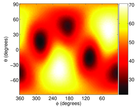
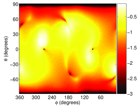
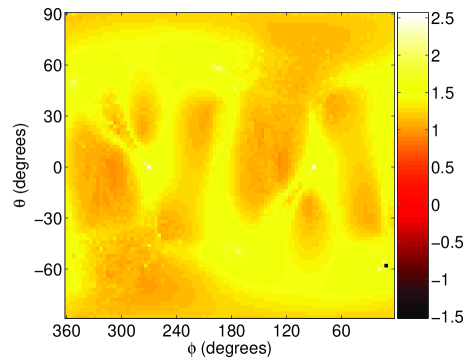
The resulting Fisher matrix is well-behaved everywhere in the five-dimensional sub-space except on a set of points of measure zero, where the detectors in the network cease to be geometrically independent. Its inverse yields the error estimates for the two mass parameters and the sky-position. A sky-map of the network SNR is presented in Fig. 14 while the sky-maps of the errors in the source luminosity-distance and the sky-position are given in Fig. 15 for equal-mass BBH sources with M=100$M_{\odot}$ and located at $d_{L}=1$Gpc.

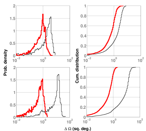
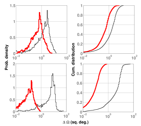
Figure 16 shows the all-sky distribution of the errors in estimating the solid angle $\Omega$. The left plots show the probability density and the right plots show the cumulative distribution. We assume that the sources are distributed uniformly across the sky. Top panels correspond to a binary with $M=20M_{\odot}$ and $\eta=0.25$, and the bottom panels to a binary with $M=100M_{\odot}$ and $\eta=0.25$. In each plot the thick (red) traces correspond to the errors estimated using the complete waveforms while the thin (black) traces correspond to those estimated using restricted 3.5PN waveforms in the SPA truncated at Schwarzschild ISCO. All the errors are computed for a network SNR of 10 for the respective waveforms. The error-estimates are obtained by averaging over the angles $(\psi,\iota)$. These plots show that in the case of an $M=20M_{\odot}$ and $\eta=0.25$ binary, assuming that the sources are distributed uniformly across the sky, the sky-position of 70% [10%] of the sources can be estimated with an accuracy better than 1 [0.1] square degree. Using PN templates, the sky-location of only 29% [6%] of the sources can be estimated with an accuracy better than 1 [0.1] square degree. For the $M=100M_{\odot}$ binary, the sky-position of 90% [18%] of the sources can be estimated with an accuracy of 1 [0.1] square degree using complete waveforms, while only 15% [4%] of the sources can be resolved with the same accuracy using inspiral waveforms. It should be noted that in that figure we have normalized the errors for SNR fixed to 10. For real systems additional improvement might be seen from the use of the complete waveforms provided their inclusion of merger and ringdown phases actually improves the SNR of those signals. This is indeed the case for high-mass systems ($M>20M_{\odot}$). For an equal-mass binary with $M=20\,[100]\,M_{\odot}$, the improvement in the SNR by the inclusion of merger and ringdown is $9\%\,[300\%]$, in stationary, Gaussian noise. (See the discussion of Fig. 18 below.)

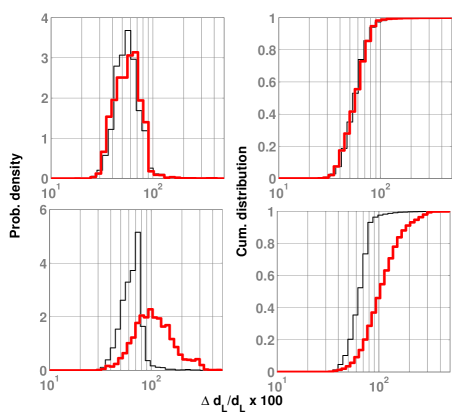
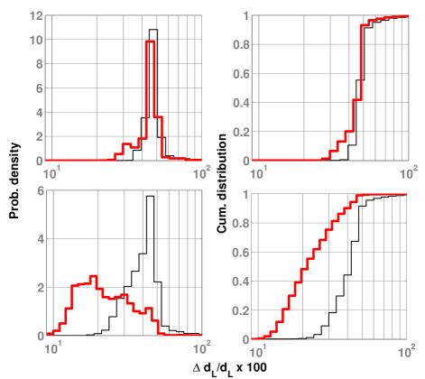
Figure 17 shows the distribution of the errors in estimating the luminosity distance $d_{L}$ to two different types of equal-mass binary systems, both producing a network SNR of 10 in the AdvLIGO-AdvVirgo network. The top panels correspond to a binary with $M=20M_{\odot}$ and the bottom panel to a binary with $M=100M_{\odot}$. As in Fig. 16, the thick (red) traces correspond the complete waveforms while the thin (black) traces correspond to the PN waveforms. These plots suggest that for an SNR of 10 the luminosity distance to around $10\%[50\%]$ of the sources can be estimated with an accuracy of better than $38\%[53\%]$ in the case of low-mass systems. They also reveal that, for a fixed value of the network SNR, the error estimates using inspiral and complete waveforms are almost identical. This is not surprising because for low-mass systems the signal is dominated by the inspiral phase. In the case of high-mass systems with an SNR of 10, the luminosity distance to around $10\%[50\%]$ of the sources can be estimated with an accuracy of $60\%[100\%]$. These errors are worse than those for the PN waveform  primarily because the covariances between the initial phase and $(\psi,\iota)$ are stronger in the case of complete waveforms. This property of the complete waveforms mitigates the estimation accuracy of $\iota$, which, in turn, affects the estimation of $d_{L}$.

Figures 18 and 19 show the errors in estimating $\Omega$ and $d_{L}$ in the case of binaries distributed uniformly across the sky but located at a luminosity distance of 1Gpc. These errors also are averaged over $\psi$ and $\iota$. These plots show that in the case of an equal-mass binary with $M=20M_{\odot}$ the sky-position of around $10\%[50\%]$ of the sources can be estimated with a resolution of $0.07[0.5]$ square degree or better. In the case of a $M=100M_{\odot}$ binary, 10%[50%] of the sources can be estimated with a resolution of 0.01[0.1] square degrees. These plots in Fig. 18 also show that the coherent addition of the merger and ringdown phases brings about remarkable improvement (i.e., by several times for most sky-positions) in the estimation of $\Omega$.

Figure 19 shows that the luminosity distance of $10\%[50\%]$ of the $M=20M_{\odot}$ BBH sources can be estimated with $32\%[47\%]$ accuracy or better and that of 10%[50%] of the $M=100M_{\odot}$ binaries can be estimated with an accuracy of 13%[20%] or better. While comparing Figs. 17 and 19, it may help to track the mean errors listed in Table 2. Studying these plots and numbers reveals some interesting aspects of these signals. First, for the PN waveforms the distance error improves only slightly in going from an SNR of 10 to a source distance of 1Gpc. This is easily explained by the fact that the sky-averaged SNR of these systems at $d_{L}$=1Gpc is only slightly greater than 10. Second, the distance error reduces a little for complete waveforms vis à vis inspiral ones at 1Gpc. This is mainly due to the increased SNR of the former. Third, the error for the complete waveforms for the $M=100M_{\odot}$ system at 1Gpc is still the smallest of all the cases studied here because its sky-averaged SNR is sufficiently large; indeed, it is large enough to even compensate for the increased covariance between $\varphi_{0}$ and $(\psi,\iota)$ arising from the merger and ringdown phases, as discussed above.

	$\rho=10$		$d_{L}=1\mathrm{Gpc}$
$M/M_{\odot}$	$\Delta\Omega$	$\Delta d_{L}/d_{L}$	$\Delta\Omega$	$\Delta d_{L}/d_{L}$
20	0.78 (2.2)	55.7% (55.3%)	0.70 (2.1)	43.2% (46.8%)
100	0.55 (8.9)	111% (63.1%)	0.13 (5.9)	23.0% (39.8%)

Table 2: Sky-averaged errors in estimating $\Omega$ and $d_{L}$ using complete BBH waveforms in the case of AdvLIGO-AdvVirgo network. The left column tabulates the errors corresponding to a fixed value $\rho=10$ for the network SNR, while the right column tabulates the errors corresponding to a fixed value $d_{L}=\mathrm{1Gpc}$ of the luminosity distance. Errors computed using PN templates are shown in parentheses. The $\Omega$ errors are given in square degrees and the fractional $d_{L}$ errors are given in percentage.

Finally, we compare our results with a couple of past studies in the form of Refs. Cutler and Flanagan (1994); Jaranowski et al. (1996). First, both these early studies used the same noise PSD for both LIGO and Virgo detectors. Second, their noise PSD was different from both the AdvLIGO and the AdvVirgo noise PSDs used here; it made their detectors more sensitive (by a factor of a few in amplitude) in the band below 70Hz and somewhat less sensitive at higher frequencies than the AdvLIGO PSD used here. Third, they considered only inspiral signals from binary neutron stars with a component mass of 1.4$M_{\odot}$, and distributed them uniformly across a spatial volume. Fourth, in Ref. Jaranowski et al. (1996) the authors culled every source that gave a distance error of greater than 100% or that had an SNR of less than 8.5. In our study, where all sources were kept at a fixed distance of 1Gpc, none of them were culled. Also, whereas all our sources with $M=100~{}M_{\odot}$ have an SNR greater than about 25, those with $M=20~{}M_{\odot}$ have the smallest SNR equal to 6. These differences make it difficult to compare these different studies. It is, however, possible to make some limited comparisons. Specifically, Fig. 15 in Ref. Jaranowski et al. (1996) suggests that the fractional errors in the estimated source distances all tend to be greater than 100% as their source distance approaches 1Gpc. Figure 14 of Ref. Cutler and Flanagan (1994) depicts a similar trend. This appears to be consistent with our numbers.

V Summary

In this paper, we studied the statistical errors in estimating the parameters of non-spinning BH binaries using ground-based GW observatories. Our study was restricted to the leading harmonic of the GW polarizations of such sources; but employing waveforms modelling the inspiral, merger and ring-down stages of the binary coalescence. We obtain results both for single- and multi-detector searches. The single-detector problem was investigated in the context of two generations of ground-based detectors, namely, Initial LIGO and Advanced LIGO, as well as Enhanced LIGO, with intermediate sensitivity. On the other hand, the multi-detector problem was investigated in the context of the Advanced LIGO-Advanced Virgo network. For these calculations, we adopted a two-pronged approach: We first analytically computed the error bounds using the Fisher-matrix formalism. We then pointed out the limitations of this approach and improved upon those calculations by full-fledged Monte-Carlo simulations.

To summarize, we find that with an Advanced LIGO detector the total mass of an equal-mass binary with $M=20M_{\odot}[100M_{\odot}]$ located at 1 Gpc can be estimated with an accuracy of $\sim 0.67[\sim 0.34]\%$, while its symmetric mass ratio can be estimated with an accuracy of $\sim 1.26[\sim 0.84]\%$. The effective distance can be estimated with an accuracy of $\sim 4.87[\sim 1.36]\%$ and the time-of-arrival can be placed within $\sim 0.11[\sim 0.46]$ ms. We considered binaries with three different mass ratios ($\eta=0.25,0.2222,0.16$) in the range $10M_{\odot}\leq M\leq 450M_{\odot}$ for these calculations. These results predict for a significantly more accurate astrophysical characterization than what has been presented in the past literature (which use the post-Newtonian waveforms intended to model only the inspiral stage of the binary). To wit, the error-bounds for total mass, computed using the complete waveforms is better than those computed using the inspiral-only waveforms by a factor of $\sim 1.4\,[\sim 16]$ for an equal-mass binary with total mass $20M_{\odot}[100M_{\odot}]$. The error-bounds on the symmetric mass ratio is improved by a factor of $\sim 1.4\,[\sim 15]$, those on the time-of-arrival is improved by a factor of $\sim 7\,[\sim 34]$ and those on the effective distance is improved by a factor of $\sim 1.1\,[\sim 4]$ by the inclusion of the merger and ringdown stages.

In the case of a network consisting of two Advanced LIGO detectors and one Advanced Virgo detector, we found that the luminosity distance to an equal-mass binary with $M=20M_{\odot}$ at 1Gpc can be estimated with a sky- and orientation-averaged accuracy of 43.2% and the sky location can be estimated with a mean accuracy of 0.7 square degrees. For a similar binary, but with $M=100M_{\odot}$, the respective mean accuracies are 23% and 0.13 square degrees. For low-mass binaries, with $(M\sim 20M_{\odot})$, the improvement in the sky-position accuracy due to the inclusion of merger and ringdown is about a factor of 3, while for high-mass binaries $(M\sim 100M_{\odot})$, that improvement is by a factor of 45. The inclusion of the same two phases betters the distance estimates by a few (for low mass systems) to several (for high mass systems) percent. In short, the sky resolution is greatly improved by the inclusion of merger and ringdown, while the improvement in the estimation of the luminosity distance arises largely from the extra SNR contributed by the merger and ringdown.

In the case of the AdvLIGO-AdvVirgo detector network, the parameter-estimation accuracy peaks for binaries with $M\simeq 100M_{\odot}$. Although the observational evidence for BHs in this mass range is only suggestive, there is growing consensus in the astronomy community that IMBHs could exist in dense stellar clusters. The existence of this class of black holes could explain a number of observations, such as the ultraluminous X-ray sources and the excess dark matter concentration in globular clusters.

Several authors have considered the scenario of the coalescence of IMBHs and have come up with coalescence-rate predictions Mandel et al. (2007); Amaro-Seoane and Freitag (2006). Particularly interesting is the case of the merger of two stellar clusters each hosting an IMBH considered in Ref. Amaro-Seoane and Freitag (2006). Since this is expected to be a strong source of GW signal with a possible EM counterpart , it is a worthwhile question to ask what kind of constraints can be put on the values of cosmological parameters by combining GW and EM observations of such sources Schutz (1986). The improved parameter estimation might help to tighten these constraints. This is being investigated in an ongoing work Ajith and Bose (2008).