Physisorption kinetics of electrons at plasma boundaries

Abstract

Plasma-boundaries floating in an ionized gas are usually negatively charged. They accumulate electrons more efficiently than ions leading to the formation of a quasi-stationary electron film at the boundaries. We propose to interpret the build-up of surface charges at inert plasma boundaries, where other surface modifications, for instance, implantation of particles and reconstruction or destruction of the surface due to impact of high energy particles can be neglected, as a physisorption process in front of the wall. The electron sticking coefficient $s_{e}$ and the electron desorption time $\tau_{e}$, which play an important role in determining the quasi-stationary surface charge, and about which little is empirically and theoretically known, can then be calculated from microscopic models for the electron-wall interaction. Irrespective of the sophistication of the models, the static part of the electron-wall interaction determines the binding energy of the electron, whereas inelastic processes at the wall determine $s_{e}$ and $\tau_{e}$. As an illustration, we calculate $s_{e}$ and $\tau_{e}$ for a metal, using the simplest model in which the static part of the electron-metal interaction is approximated by the classical image potential. Assuming electrons from the plasma to loose (gain) energy at the surface by creating (annihilating) electron-hole pairs in the metal, which is treated as a jellium half-space with an infinitely high workfunction, we obtain $s_{e}\approx 10^{-4}$ and $\tau_{e}\approx 10^{-2}s$. The product $s_{e}\tau_{e}\approx 10^{-6}s$ has the order of magnitude expected from our earlier results for the charge of dust particles in a plasma but individually $s_{e}$ is unexpectedly small and $\tau_{e}$ is somewhat large. The former is a consequence of the small matrix elements occurring in the simple model while the latter is due to the large binding energy of the electron. More sophisticated theoretical investigations, but also experimental support, are clearly needed because if $s_{e}$ is indeed as small as our exploratory calculation suggests, it would have severe consequences for the understanding of the formation of surface charges at plasma boundaries. To identify what we believe are key issues of the electronic microphysics at inert plasma boundaries and to inspire other groups to join us on our journey is the purpose of this colloquial presentation.

1 Introduction

Low-temperature plasma physics is undoubtedly an applied science driven by the ever increasing demand for plasma-assisted surface modification processes and environmentally save, low-power consuming lighting devices. At the same time, however, the physics of gas discharges is rich on fundamental problems which are of broader interest.

From a formal point of view, a gas discharge is an externally driven bounded reactive multicomponent system. It contains, besides electrons and ions, chemically reactive atoms and/or molecules strongly interacting with each other and with external (wall of the discharge vessel) as well as internal ($nm$ to $\mu m$-sized solid particles) boundaries. Like in any reactive system elementary collision processes (elastic, inelastic, and reactive), occurring on a microscopic scale, determine in conjunction with external control parameters the global properties of the system on the macroscopic scale. However, whereas in an ordinary chemical reactor all constituents are neutral, a gas discharge contains also charged constituents. There are thus at least two macroscopic scales: the electromagnetic scale, where screening and sheath formation takes place Franklin06 ; Riemann91 , and the extension of the vessel. Since the observed physical properties of a gas discharges emerge from processes occurring on at least three different length (and time) scales – one microscopic and two macroscopic scales – the starting point of any quantitative description is a multiple-scale analysis even if it is not explicitly performed. Being externally driven, low-temperature plasmas are moreover far-off thermal equilibrium and like other dissipative systems feature a great variety of self-organization phenomena Purwins08 ; PBL04 . Finally, and this sets the theme of this colloquium, low-temperature gas discharges, in contrast to magnetically confined high-temperature fusion plasmas, are directly bounded by massive macroscopic objects. Thus, they strongly interact with solids.

The plasma-solid interaction is of course at the core of all plasma-assisted surface processes (deposition, implantation, sputtering, etching, etc.) LL05 . Of more fundamental interest, however, is the situation of a chemically inert (i.e., no surface modification due to chemical processes, no reconstruction or destruction of the surface due to high-energy particles etc.) floating surface, where the interaction with the plasma leads only to the build-up of surface charges and thus to a quasi-two-dimensional electron film which may have unique properties similar to electrons trapped on a liquid helium surface Cole74 or to electrons confined in a semiconductor heterojunction AFS82 .

In plasma-physical settings surface charges play a role in atmospheric plasmas, where the charge of $nm$-sized aerosols RL01 is of interest, in space bound plasmas, where surface charges of spacecrafts GW00 ; Whipple81 and of interplanetary and interstellar dust particles Mann08 ; Horanyi96 have been extensively studied, and in laboratory dusty plasmas, where the study of self-organization of highly negatively charged, strongly interacting $\mu m$-sized dust particles became an extremely active area of current plasma research Ishihara07 ; FIK05 ; KRZ05 ; SV03 ; TAA00 ; TLA00 ; WHR95 . Surface charges affect also the physics of dielectric barrier discharges – a discharge type of huge technological impact GMB02 ; Kogelschatz03 ; KCO04 ; SAB06 ; SLP07 ; LLZ08 .

That surface charges at plasma boundaries could be considered as a thin film of adsorbed electrons (“surface plasma”) in contact with the bulk plasma was originally suggested by Emeleus and Coulter in connection with their investigations of wall recombination in the positive column EC87 . Later, Behnke and coworkers BBD97 used this idea to phenomenologically construct boundary conditions for the kinetic equations describing glow discharges and Kersten et al. KDK04 employed the notion of a surface plasma to study the charging of dust particles in a plasma.

Although the surface plasma as a physical entity with its own physical properties is implicitly contained in these investigations, a microscopic description of its formation, dynamics, and structure was not attempted. First steps in this direction were taken by us in a short note BFK08 . The purpose of this colloquium is, on the one hand, to extend these considerations, in particular, to identify the surface physics which needs to be resolved before a quantitative microscopic theory of the surface plasma can be constructed and to convey, on the other hand, our conviction that the concept itself is not empty. On the contrary, it puts questions center stage which are of fundamental interest. To list just a few:

$\bullet$	What forces bind electrons and ions to the plasma
	boundary?
$\bullet$	How do electrons and ions dissipate energy when
	approaching the boundary?
$\bullet$	What is the probability with which an electron sticks
	at or desorbs from the boundary?
$\bullet$	What is the density and temperature of the surface
	plasma and are there any collective properties?
$\bullet$	What is the mobility for the lateral motion of
	electrons and ions along the wall and can it be
	externally controlled?
$\bullet$	How does all this affect electron-ion recombination
	and secondary electron emission on chemically inert
	plasma boundaries?

The elementary processes responsible for the formation of a surface plasma at an inert plasma boundary are shown in Fig 1. Electrons and ions are collected from the plasma with collection fluxes $j_{e,i}^{\rm coll}=s_{e,i}j_{e,i}^{\rm plasma}$, where $s_{e,i}$ are the sticking coefficients and $j_{e,i}^{\rm plasma}$ are the fluxes of plasma electrons and ions hitting the boundary. Electrons and ions may thermally desorb from the boundary with rates $\tau_{e,i}^{-1}$, where $\tau_{e,i}$ are the desorption times. They may also move along the surface with mobilities $\mu_{e,i}$, which in turn may affect the probability $\alpha_{R}$ with which ions recombine with electrons at the wall. All these processes occur in a layer whose thickness $d$ is at most a few microns, that is, on a scale where the standard kinetic description of the gas discharge based on the Boltzmann-Poisson system breaks down. Thus, the above listed questions can be only addressed from a quantum-mechanical point of view.

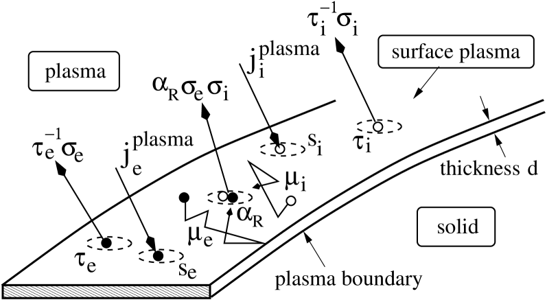
Figure 1: Illustration of the elementary surface processes leading to the build-up of a quasi-stationary surface plasma at an inert plasma boundary.

Of particular importance for the quantitative description of the build-up of a surface plasma are the sticking coefficients $s_{e,i}$ and the desorption times $\tau_{e,i}$. Little is quantitatively known about these parameters, in particular, with respect to the electrons. Very often, $s_{e}\approx s_{i}\approx 0.1-1$ and $\tau_{e}^{-1}=\tau_{i}^{-1}=0$ is used without further justification. Below, we sketch a quantum-kinetic approach to calculate $s_{e}$ and $\tau_{e}$ from a simple microscopic model for the plasma boundary interaction which treats the interaction of electrons with plasma boundaries as a physisorption process LJD36 ; BY73 ; GKT80a ; GKT80b ; KT81 ; Brenig82 ; KG86 ; NNS86 ; GS91 ; BR92 ; WJS92 in the polarization-induced attractive part of the surface potential. Electron surface states RM72 ; EM73 ; Barton81 ; DAG84 ; SH84 ; WHJ85 ; JDK86 ; EP90 ; EL94 ; Fauster94 ; EL95 ; HSR97 ; CSE99 ; Hoefer99 ; VPE07 , at most a few $nm$ away from the boundary, will thus play a central role as will surface-bound scattering processes which control electron energy relaxation at the surface and thus electron sticking and desorption.

Although the forces and scales are different for ions, they behave conceptually very similar. The main difference between electrons and ions is that as soon as the surface collected some electrons, because of the faster bombardment with electrons than with ions, the surface potential for ions is the attractive Coulomb potential (most probably screened but thats for the following irrelevant). Hence, ion surface states develop in the tail of the long-ranged Coulomb potential and thus deep in the sheath of the grain, far away from its surface. The microscopic processes driving ion energy relaxation and eventually ion sticking and desorption are thus not surface- but plasma-bound.

In the microscopic approach presented below, we focus on the physics occurring at most a few $nm$ away from the boundary. We will therefore not give here a quantitative treatment of the physisorption kinetics of ions in the long-ranged Coulomb potential. However, when it comes to the calculation of the surface charge via phenomenological equations connecting the quantum with the classical level, we have to make some assumptions about the ion dynamics and kinetics. We will then discuss ions qualitatively. The assumptions made for ions, which are somewhat in conflict with what other people expect LGG01 ; LGS03 ; SLR04 , do however not affect the microscopic calculation of $s_{e}$ and $\tau_{e}$.

The outline of this colloquium is as follows. In the next section we describe and put into context the surface model for the charge of a floating dust particle in a plasma we developed in BFK08 because it motivated the physisorption-inspired microscopic treatment of electrons at plasma boundaries discussed in this colloquium. A qualitative description of the ion kinetics in the vicinity of a spherical grain is also included in this section. Section 3 describes a microscopic model for the interaction of electrons with plasma boundaries. Specified to a metallic boundary, it will then be used to calculate the electron sticking coefficient $s_{e}$ and the electron desorption time $\tau_{e}$. Key issues of the microscopic description of the electron-wall interaction (surface potential, coupling to elementary excitations of the solid, etc.) will be identified and numerical results will be presented and discussed. A critique of our assumptions is given at the end of section 3 and should be understood as a list of to-do’s. We close the presentation in section 4 with a few concluding remarks. Mathematical details interrupting the presentation which is meant to be read in order because it successively constructs a case are relegated to three appendices.

2 Charge of a dust particle in a plasma

The physisorption-inspired treatment of surface charges originated from our attempt to calculate the charge of a spherical $\mu m$-sized floating dust particle in a quiescent plasma, taking not only plasma-induced but also surface-induced processes into account BFK08 . Here we have to clearly distinguish between the assumptions made to construct a constituting equation for the surface charge, which by necessity has to connect the quantum mechanics occurring at the surface with the classical physics determining the plasma fluxes, and the assumptions to obtain estimates for the surface parameters appearing in this equation. The microscopic calculation of the electron surface parameters $s_{e}$ and $\tau_{e}$ presented in the next sections is of course independent of the assumptions about the ion dynamics and kinetics as well as the phenomenological nature of the constituting equation for the surface charge.

2.1 Rate equations

First, we will discuss the surface model proposed in BFK08 from the perspective of the rate equations corresponding to the elementary processes shown in Fig. 1. Thereby we also identify the assumptions, in particular, with respect to the surface properties, which are usually made in standard calculations of surface charges.

To be specific let us consider a spherical dust particle with radius $R$. The quasi-stationary charge of the grain is given by (we measure charge in units of $-e$)

$$Z_{p}=4\pi R^{2}\big{[}\sigma_{e}-\sigma_{i}\big{]}~{},$$ (1)

with electron and ion surface densities, $\sigma_{e,i}$, satisfying the quasi-stationary ($d\sigma_{e,i}/dt=0$) rate equations KDK04 ,

$$0 = s_{e}j^{\rm plasma}_{e}-\tau_{e}^{-1}\sigma_{e}-\alpha_{R}\sigma_{e}\sigma_{i}~{},$$ (2)

$$0 = s_{i}j^{\rm plasma}_{i}-\tau_{i}^{-1}\sigma_{i}-\alpha_{R}\sigma_{e}\sigma_{i}~{},$$ (3)

where $j^{\rm plasma}_{e,i}$, $s_{e,i}$, $\tau_{e,i}$, and $\alpha_{R}$ denote, respectively, the fluxes of electrons and ions hitting the grain surface from the plasma, the electron and ion sticking coefficients, the electron and ion desorption times, and the electron-ion recombination coefficient. 

In order to derive the standard criterion invoked to determine the quasi-stationary grain charge, we now assume, in contrast to what we do in our model BFK08 (see also below), that both electrons and ions reach the surface of the grain. In that case, both Eq. (2) and Eq. (3) should be interpreted as flux balances on the grain surface. At quasi-stationarity, the grain is charged to the floating potential $\bar{U}$. In energy units, $\bar{U}=Z_{p}e^{2}/R=2Z_{p}R_{0}a_{B}/R$ with $R_{0}$ the Rydberg energy and $a_{B}$ the Bohr radius. Because the grain temperature $k_{B}T_{s}\ll\bar{U}$ the ion desorption rate $\tau_{i}^{-1}\approx 0$. Equation (3) reduces therefore to $\alpha_{R}\sigma_{e}\sigma_{i}=s_{i}j^{\rm plasma}_{i}$ which transforms Eq. (2) into $s_{e}j^{\rm plasma}_{e}=s_{i}j^{\rm plasma}_{i}+\tau_{e}^{-1}\sigma$ provided $\sigma\approx\sigma_{e}$ which is usually the case. In the standard approach the grain surface is moreover assumed to be a perfect absorber for both electrons and ions. Thus, $s_{e}=s_{i}=1$ and $\tau^{-1}_{e}=\tau_{i}^{-1}=0$. The quasi-stationary charge $Z_{p}$ of the grain is then obtained from the condition

$$j^{\rm plasma}_{e}(Z_{p})=j^{\rm plasma}_{i}(Z_{p})~{},$$ (4)

where we explicitly indicated the dependence of the plasma fluxes on the grain charge.

Calculations of the grain charge differ primarily in the approximations made for the plasma fluxes $j_{e,i}^{\rm plasma}$. For the repelled species, usually collisionless electrons, the flux can be obtained from Poisson’s equation and the collisionless Boltzmann equation, using trajectory tracing techniques based on Liouville’s theorem and energy and momentum conservation BR59 ; LP73 ; DPK92 . The flux for the attracted species, usually collisional ions, is much harder to obtain. Unlike the electron flux, the ion flux depends not only on the field of the macroscopic body but also on scattering processes due to the surrounding plasma, which throughout we assume to be quiescent. For weak ion collisionalities the charge-exchange enhanced ion flux model proposed by Lampe and coworkers LGG01 ; LGS03 ; SLR04 is usually used. Its validity has been however questioned by Tskhakaya and coworkers TTS01 ; TSS01 . We come back to Lampe and coworkers approach below when we discuss representative results for our surface model.

Hence, irrespective of the approximations made for the plasma fluxes, the standard approach of calculating surface charges is based on three assumptions about the surface physics:

$\bullet$	Both ions and electrons reach the surface, even on the
	microscopic scale.
$\bullet$	$s_{e}=s_{i}=1$ or at least $s_{e}=s_{i}$.
$\bullet$	$\tau_{e}^{-1}=0$ or at least $\tau_{e}^{-1}\sigma_{e}\ll s_{i}j_{i}^{\rm plasma}=\alpha_{R}\sigma_{e}\sigma_{i}.$

We basically challenge all three assumptions.

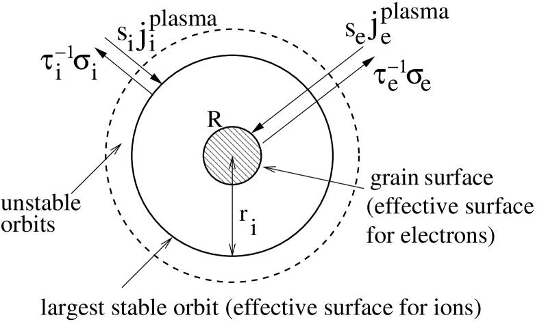
Figure 2: Illustration of the surface model for the charging of a dust particle with radius $R$ in a gas discharge. At quasi-stationarity, surface charges $\sigma_{e,i}$ bound at $r_{e}\approx R$ and $r_{i}\gtrsim r_{e}$, respectively, balance the collection flux $s_{e,i}j^{\rm plasma}_{e,i}$ with the respective desorption flux $\tau_{e,i}^{-1}\sigma_{e,i}$, where $s_{e,i}$ and $\tau_{e,i}$ denote, respectively, sticking coefficients and desorption times BFK08 .

First, electrons and ions should be bound in surface states. Because of differences in the potential energy, mass, and size the spatial extension of the electron and ion bound states, and thus the average distance of electrons and ions from the boundary, is expected to be different. On the microscopic scale, electrons and ions trapped to the surface should be spatially separated.

Second, $s_{e}=s_{i}$ is quite unlikely. Usually, heavy particles, such as ions, couple rather strongly to vibrational excitations of the boundary KG86 ; BR92 . They can thus dissipate energy very efficiently which usually leads to a large sticking coefficient. Light particles, like electrons, on the other hand, couple only very weakly to vibrations of the solid. On this basis, we would expect $s_{e}\ll s_{i}$. To what extend the coupling to other elementary excitations of the boundary (plasmons, electron-hole pairs, …) can compensate for the inefficient coupling to lattice vibrations is part of our investigations.

Third, if ions and electrons are indeed spatially separated, the two rate equations should be in fact interpreted as flux balances on two different effective surfaces (viz: the two closed circles in Fig. 2). In that case, $\alpha_{R}\sigma_{i}\sigma_{e}\ll\sigma_{e,i}/\tau_{e,i}$ and the surface charge $Z_{p}$ would be determined by balancing on the grain surface the electron desorption flux, $\tau_{e}^{-1}\sigma_{e}$, with the electron collection flux, $s_{e}j_{e}^{\rm plasma}$. The corresponding balance of ion fluxes, to be taken on an effective surface surrounding the grain, would then yield a partial screening charge $Z_{i}$. Within this scenario, we would thus obtain

$$Z_{p} = 4\pi r_{e}^{2}\cdot(s\tau)_{e}\cdot j_{e}^{\rm plasma}(Z_{p})~{},$$ (5)

$$Z_{i} = 4\pi r_{i}^{2}\cdot(s\tau)_{i}\cdot j_{i}^{\rm plasma}~{},$$ (6)

with $r_{e}\approx R$ and $r_{i}\gtrsim r_{e}$.

The surface physics is now encoded in $(s\tau)_{e,i}$. These products depend on the material and the plasma. They could be used as adjustable parameters. A justification of the assumptions, however, made in deriving Eqs. (5) and (6) can only come from a microscopic calculation of $(s\tau)_{e,i}$.

For electrons, various aspects of this calculation will be discussed in the following sections.

2.2 Semi-microscopic approach

Before we discuss the complete microscopic calculation of $s_{e}$ and $\tau_{e}$ we summarize the semi-microscopic approach taken in Ref. BFK08 . This prepares the grounds for a microscopic thinking and demonstrates that Eqs. (5) and (6) give results which compare favorable with experimental data.

The approach we adopted in Ref. BFK08 is based on a quantum mechanical investigation of the bound states of a negatively charged particle in a gas discharge. For that purpose, we considered the classical interaction between an electron (ion) with charge $-e$ ($+e$) and a spherical particle with radius $R$, dielectric constant $\epsilon$, and charge $Z_{p}$. The interaction potential contains then a short-ranged polarization-induced part arising from the electric boundary conditions at the grain surface – the classical image potential – and a long-ranged Coulomb tail due to the particle’s charge Boettcher52 ; DS87 .

The polarization-induced part of the potential will be discussed from a quantum-mechanical point of view in appendix A. Concerning the Coulomb tail we may add that it arises from the interaction between the approaching electron and the electrons already residing on the grain. From many-body theory it is known that this interaction can be rather involved because the attached electrons may respond dynamically VR93 . We neglect this possibility. The Coulomb part is then simply the potential of a sphere (plane) with charge $Z_{p}$. This is equivalent to a meanfield approximation for the electron-electron interaction.

Measuring distances from the grain surface in units of $R$ and energies in units of $\bar{U}$, the interaction energy at $x=r/R-1>x_{b}$, where $x_{b}$ is a lower cut-off, below which the grain boundary cannot be described as a perfect surface anymore, reads

$$V_{e,i}(x) = \pm\frac{1}{1+x}-\frac{\xi}{x(1+x)^{2}(2+x)}$$ (9)

$$\approx \left\{\begin{array}[]{ll}1-\xi/2x&\mbox{electron}\\ -1/(1+x)&\mbox{ion}\end{array}\right.$$

with $\xi=(\epsilon-1)/2(\epsilon+1)Z_{p}$.

The second line in Eq. (9) is an approximation which describes the relevant parts of the potential very well and permits an analytical calculation of the surface states. In Fig. 3 we plot $V_{e,i}(x)$ for a melamine-formaldehyde (MF) particle ($\epsilon=8$, $R=1~{}\mu m$, and $Z_{p}=1500$) embedded in a $100Pa$ neon discharge with plasma density $n_{e}=n_{i}=0.39\times 10^{9}~{}cm^{-3}$, ion temperature $k_{B}T_{i}=0.026~{}eV$, and electron temperature $k_{B}T_{e}=6.3~{}eV$ KRZ05 . From the electron energy distribution, $f_{e}(E)$, we see that the discharge contains enough electrons which can overcome the Coulomb barrier of the dust particle. These electrons may get bound in the polarization-induced short-range part of the potential, well described by the approximate expression, provided they can get rid of their kinetic energy. Ions, on the other hand, being cold (see $f_{i}(E)$ in Fig. 3) and having a finite radius $r^{size}_{i}/R=x_{i}^{size}\gtrsim 10^{-4}$, cannot explore the potential at short distances. For them, the long-range Coulomb tail is most relevant, which is again well described by the approximate expression.

Writing for the electron eigenvalue $\varepsilon^{e}=1-\alpha_{e}\xi/4k^{2}$ with $\alpha_{e}=(\epsilon-1)R/4(\epsilon+1)a_{B}$ and for the ion eigenvalue $\varepsilon^{i}=-\alpha_{i}/2k^{2}$ with $\alpha_{i}=m_{i}RZ_{p}/m_{e}a_{B}$, where $m_{e}$ and $m_{i}$ are the electron and ion mass, respectively, the radial Schrödinger equations with the approximate potentials read

$$\frac{d^{2}u^{e,i}}{dx^{2}}+\bigg{[}-\frac{\alpha_{e,i}^{2}}{k^{2}}+\tilde{V}_{e,i}(x)-\frac{l(l+1)}{(1+x)^{2}}\bigg{]}u^{e,i}=0$$ (10)

where $\tilde{V}_{e}(x)=2\alpha_{e}/x$ and $\tilde{V}_{i}(x)=2\alpha_{i}/(1+x)$.

For bound states, the wavefunctions have to vanish for $x\rightarrow\infty$. The boundary condition at $x_{b}$ depends on the potential for $x\leq x_{b}$, that is, on the potential within the solid (which is different for electrons and ions). Matching the solutions for $x<x_{b}$ and $x>x_{b}$ at $x=x_{b}$ leads to a secular equation for $k$. Ignoring the possibility that electrons and ions may also enter the solid, we set $\tilde{V}_{e,i}(x\leq x_{b})=\infty$ with $x_{b}=0$ for electrons and $x_{b}=x_{i}^{size}$ for ions. For electrons we thereby restrict ourselves to weakly bound polarization-induced surface states, neglecting strongly bound crystal-induced surface states which, in general, may also occur Spanjaard96 . As explained in the next section, we expect them to be of minor importance for physisorption of electrons.

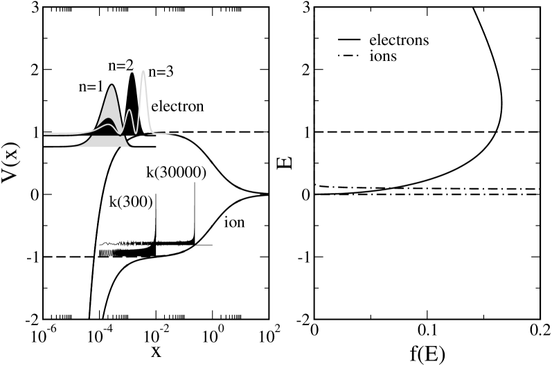
Figure 3: Left panel: Potential energy for an electron (ion) in the field of a MF particle ($R=1~{}\mu m$, $Z=1500$) KRZ05 and representative probability distributions, $|u(x)|^{2}$, shifted to the binding energy and maxima normalized to one. Dashed lines denote the potentials used in the Schrödinger equations. Note, the finite ion radius $r_{i}^{size}\sim\AA$ forces the ion wavefunctions to vanish at $x\approx 10^{-4}$. Right panel: Bulk energy distribution functions for the $100Pa$ neon discharge hosting the particle KRZ05 : $k_{B}T_{e}=6.3eV$, $k_{B}T_{i}=0.026eV$, and $n_{e}=n_{i}=0.39\times 10^{9}cm^{-3}$.

The electron Schrödinger equation with the hard boundary condition at $z=0$ is equivalent to the radial Schrödinger equation for the hydrogen atom. Hence $k$ is an integer $n$. Because (for bound electrons) $x\ll 1$ and $\alpha_{e}\gg 1$, the centrifugal term is negligible. We consider therefore only states with $l=0$. The eigenvalues are then $\varepsilon^{e}_{n}=1-\alpha_{e}\xi/4n^{2}$ and the wavefunctions read

$$u_{n,0}^{e}(x) \sim v_{n,0}(\bar{z})$$ (11)

$$= \bar{z}\exp(-\bar{z}/2)(-)^{n-1}(n-1)!L^{(1)}_{n-1}(\bar{z})$$

with $\bar{z}=2\alpha_{e}x/n$ and $L^{(1)}_{n}(\bar{z})$ associated Laguerre polynomials.

The probability densities $|u_{n,0}^{e}(x)|^{2}$ for the first three states are plotted in Fig. 3. As can be seen, electron surface states are only a few $\AA$ngstroms away from the grain boundary. At these distances, the spatial variation of $V_{e}(x)$ is comparable to the de-Broglie wavelength of electrons approaching the particle. More specifically, for $k_{B}T_{e}=6.3~{}eV$, $\lambda_{e}^{dB}/R\approx|V_{e}/V_{e}^{\prime}|\approx 10^{-4}$. Hence, the trapping of electrons at the surface of the particle has to be described quantum-mechanically.

The solutions of the ion Schrödinger equation are Whittaker functions, $u^{i}_{k,l}(x)=W_{k,l+1/2}(\bar{x})$ with $\bar{x}=2\alpha_{i}(1+x)/k$ and $k$ determined from $u^{i}_{k,l}(x_{i}^{size})=0$. However, since $k\gg 1$ and $\bar{x}\gg 1$, it is very hard to work directly with $W_{k,l+1/2}(\bar{x})$. It is easier to use the method of comparison equations Richardson73 and to construct uniform approximations for $u^{i}_{k,l}(x)$ with the radial Schrödinger equation for the hydrogen atom as a comparison equation. The method can be applied for any $l$. Here we give only the result for $l=0$:

$$u_{k,0}^{i}(x)\sim v_{n,0}(\bar{z})/\sqrt{dz/dx}$$ (12)

with $v_{n,0}(\bar{z})$ defined in Eq. (11) and $\bar{z}=2\alpha_{i}z(x)/n$. The mappings $z(x)$ and $k(n)$ can be constructed from the phase-integrals of the two Schrödinger equations.

In Fig. 3 we show $|u_{k,0}^{i}(x)|^{2}$ for $k(300)$ and $k(30000)$. Note, even the $k(30000)$ state is basically at the bottom of the potential. This is a consequence of $\alpha_{i}\gg 1$ which leads to a continuum of states below the ion ionization threshold at $\varepsilon=0$. We also note that $|u_{k(n),0}^{i}(x)|^{2}$ peaks for $n\gg 1$ just below the turning point. Hence, except for the lowest states, which we expect to be of little importance, ions are essentially trapped in classical orbits deep in the sheath of the grain. This will be also the case for $l>0$. That ions behave classically is not unexpected because for $k_{B}T_{i}=0.026~{}eV$ their de-Broglie wavelength is much smaller then the scale on which the potential varies for $x>10^{-3}$: $\lambda_{i}^{dB}/R\approx 10^{-5}\ll|V_{i}/V_{i}^{\prime}|\approx 1$. Thus, the interaction between ions and the particle is classical.

Nevertheless it can be advantageous to describe ions quantum-mechanically and to use the method of comparison equations, which is an asymptotic technique, to perform the calculation in the semiclassical regime. Since the ion dynamics and kinetics is beyond the scope of this paper, we do not give more mathematical details about the solution of the ion Schrödinger equation. We mention however that many years ago Liu Liu69 pursued a quantum-mechanical description of the collisionless ion dynamics around electric probes. But he found no followers.

A model for the charge of the grain which takes surface states into account can now be constructed as follows. Within the sheath of the particle, the density of free electrons (ions) is much smaller than the density of bound electrons (ions). In that region, the quasi-stationary charge (again in units of $-e$) is thus approximately given by

$$Z(x)=4\pi R^{3}\!\int_{x_{b}}^{x}\!\!dx^{\prime}\big{(}1+x^{\prime}\big{)}^{2}\bigg{[}n^{b}_{e}(x^{\prime})-n^{b}_{i}(x^{\prime})\bigg{]}$$ (13)

with $x<\lambda^{D}_{i}=\sqrt{k_{B}T_{i}/4\pi e^{2}n_{i}}$, the ion Debye length, which we take as an upper cut-off, and $n^{b}_{e,i}$ the density of bound electrons and ions. For the plasma parameters used in Fig. 3, $\lambda^{D}_{i}\approx 60\mu m$. The results for the surface states presented above suggest to express the density of bound electrons by an electron surface density:

$$n^{b}_{e}(x)\approx\sigma_{e}\delta(x-x_{e})/R$$ (14)

with $x_{e}\approx x_{b}\approx 0$ and $\sigma_{e}$ the quasi-stationary solution of of Eq. (2) without the recombination term. Equation (2) is thus still interpreted as a rate equation on the grain surface. We will argue below that once the grain has collected some negative charge, not necessarily the quasi-stationary one, there is a critical ion orbit at $x_{i}\sim 1-10\gg x_{e}$ which prevents ions from hitting the particle surface. Thus, the particle charge obtained from Eq. (13) is simply $Z_{p}\equiv Z(x_{e}<x<x_{i})$. Inserting Eq. (14) into Eq. (13) and integrating up to $x$ with $x_{e}<x<x_{i}$ leads to Eq. (5), the expression for the particle charge deduced from the rate equations (2) and (3) under the assumption that ions do not reach the grain surface on the microscopic scale.

For an electron to get stuck at (to desorb from) a surface it has to loose (gain) energy at (from) the surface KG86 . This can only occur through inelastic scattering with the grain surface. To calculate the product $(s\tau)_{e}$ requires therefore a microscopic description of energy relaxation at the grain surface. This will be discussed in the next section. In Ref. BFK08 we invoked the phenomenology of reaction rate theory and approximated $(s\tau)_{e}$ by

$$(s\tau)_{e}=\frac{h}{k_{B}T_{s}}\exp\bigg{[}\frac{E_{e}^{d}}{k_{B}T_{s}}\bigg{]}~{},$$ (15)

where $h$ is Planck’s constant, $T_{s}$ is the surface temperature, and $E_{e}^{d}$ is the electron desorption energy, that is, the binding energy of the surface state from which desorption most likely occurs KG86 . The great virtue of this equation is that it relates a combination of kinetic coefficients, which depend on the details of the inelastic (dynamic) interaction, to an energy, which can be deduced from the static interaction alone. Kinetic considerations are thus reduced to a minimum. They are only required to identify the relevant temperature and the state from which desorption most probably occurs. In the next section we will show, for a particular model, how Eq. (15) can be obtained from a microscopic theory. Its range of validity will then become also clear.

Equation (5) is a self-consistency equation for $Z_{p}$. Combined with Eq. (15), and approximating the electron flux $j_{e}^{\rm plasma}$ from the plasma by the orbital motion limited flux,

$$j_{e}^{\rm OML}=n_{e}\sqrt{k_{B}T_{e}/2\pi m_{e}}\exp[-Z_{p}e^{2}/Rk_{B}T_{e}]~{},$$ (16)

which is reasonable, because, on the plasma scale, electrons are repelled from the grain surface, the grain charge is given by

$$Z_{p}=4\pi R^{2}\frac{h}{k_{B}T_{s}}e^{E_{e}^{d}/k_{B}T_{s}}j_{e}^{\rm OML}(Z_{p})~{}.$$ (17)

Thus, in addition to the plasma parameters $n_{e}$ and $T_{e}$, the charge depends on the surface parameters $T_{s}$ and $E_{e}^{d}$.

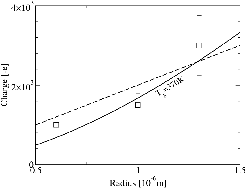
Figure 4: Radius dependence of the charge of a MF particle in the bulk of a neon discharge at $p=100Pa$ KRZ05 . The plasma parameters are the same as in Fig. 3. The solid line denotes the charges deduced from Eq. (17) and the dashed line gives the charges obtained from $j_{e}^{\rm OML}=j_{i}^{\rm OML}+j_{i}^{\rm CX}$ with $\sigma_{\rm cx}=10^{-14}cm^{-2}$.

Without a microscopic theory for the inelastic electron-grain interaction, a plausible estimate for $E_{e}^{d}$ has to be found from physical considerations alone. Since by necessity the electron comes very close to the grain surface (see Fig. 3) it will strongly couple to elementary excitations of the grain. Depending on the material these may be bulk or surface phonons, bulk or surface plasmons, or internal electron-hole pairs. For any realistic description of the potential for $x\leq x_{b}$ the electron wavefunction leaks into the solid, the electron will therefore quickly relax to the lowest surface bound state. The microscopic model for electron energy relaxation at metallic boundaries presented in the next section turns out to even work for an infinitely high barrier. Taking the $n=1$ state for $\tilde{V}_{e,i}(x\leq x_{b})=\infty$ as an approximation to the lowest surface bound state, it is reasonable to expect

$$E_{e}^{d}\approx(1-\varepsilon^{e}_{1})\bar{U}=\frac{R_{0}}{16}\bigg{(}\frac{\epsilon-1}{\epsilon+1}\bigg{)}^{2}~{},$$ (18)

which, for an MF particle with $\epsilon=8$, leads to $E_{e}^{d}\approx 0.5eV$. The particle temperature cannot be determined in a simple way. It depends on the balance of heating and cooling fluxes to-and-fro the particle and thus on additional surface parameters SKD00 . We use $T_{s}$ therefore as an adjustable parameter. To reproduce, for instance, with Eq. (17) the charge of the particle in Fig. 3, $T_{s}=370~{}K$ implying $(s\tau)_{e}\approx 10^{-6}~{}s$.

In Fig. 4 we plot the radius dependence of the charge of a MF particle in the $100Pa$ neon discharge specified in the caption of Fig. 3. More results are given in BFK08 . Since the plasma parameters are known the only adjustable parameter is the surface temperature. Using $T_{s}=370K$ we find excellent agreement between theory and experiment. For comparison we also show the charges obtained from Eq. (4), approximating the ion plasma flux by

$$j_{i}^{\rm plasma}=j_{i}^{\rm OML}+j_{i}^{\rm cx}~{},$$ (19)

where

$$j_{i}^{\rm OML}=n_{i}\sqrt{k_{B}T_{i}/2\pi m_{i}}[1+Z_{p}e^{2}/Rk_{B}T_{i}]$$ (20)

is the orbital motion limited ion flux and KRZ05

$$j_{i}^{\rm cx}=n_{i}(0.1\lambda^{D}_{i}/l_{\rm cx})\sqrt{k_{B}T_{i}/2\pi m_{i}}(Z_{p}e^{2}/Rk_{B}T_{i})^{2}$$ (21)

is the ion flux originating from the release of trapped ions due to charge-exchange scattering as suggested by Lampe and coworkers LGG01 ; LGS03 ; SLR04 . The scattering length $l_{\rm cx}=(\sigma_{\rm cx}n_{g})^{-1}$ with $\sigma_{\rm cx}=10^{-14}cm^{2}$ the scattering cross section and $n_{g}=p/k_{B}T_{g}$ the gas density. Clearly, the radius dependence of the grain charge seems to be closer to the nonlinear dependence obtained from Eq. (17) than to the linear dependence resulting from

$$j_{e}^{\rm OML}=j_{i}^{\rm OML}+j_{i}^{\rm cx}~{},$$ (22)

indicating that the surface model we propose captures at least some of the physics correctly which is responsible for the formation of surface charges.

In order to derive Eq. (17) from Eq. (13) we had to assume that once the particle is negatively charged ions are trapped far away from the grain surface. Treating trapping of ions in the field of the grain as a physisorption process suggests this assumption, which is perhaps counter-intuitive. Similar to an electron, an ion gets bound to the grain only when it looses energy. Because of its low energy and the long-range attractive ion-grain interaction, the ion will be initially bound very close to the ion ionization threshold (see Fig. 3). The coupling to the elementary excitations of the grain is thus negligible and only inelastic processes due to the plasma are able to push ions to lower bound states. Since the interaction is classical, inelastic collisions, for instance, charge-exchange scattering between ions and atoms, act like a random force. Ion energy relaxation can be thus envisaged as a de-stabilization of orbits. This is in accordance to what Lampe and coworkers assume LGG01 ; LGS03 ; SLR04 . In contrast to them, however, we BFK08 expect orbits whose spatial extension is smaller than the scattering length to be stable because the collision probability during one revolution becomes vanishingly small. For a circular orbit, a rough estimate for the critical radius is

$$r_{i}=R(1+x_{i})=(2\pi\sigma_{\rm cx}n_{g})^{-1}$$ (23)

which leads to $x_{i}\sim 5.7\gg x_{e}\sim 0$ when we use the parameters of the neon discharge of Fig. 3 and $\sigma_{\rm cx}=10^{-14}~{}cm^{2}$.

Although the approach of Lampe et al. LGG01 ; LGS03 ; SLR04 shows a pile-up of trapped ions in a shell of a few $\mu m$ radius enclosing the grain, they would not expect a relaxation bottleneck. This point can be only clarified with a detailed investigation of the ion dynamics and kinetics in the vicinity of the grain, including electron-ion recombination. As mentioned before, despite the classical character of the ion dynamics, a quantum-mechanical treatment, similar to the one we will present in the following sections for electrons, is possible and perhaps even advantageous because it treats closed (bound surface states) and open ion orbits (extended surface states) on the same footing. In addition, energy barriers due to the angular motion are easier to handle in a quantum-mechanical context. In fact, Lampe and coworkers neglect these energy barriers whereas Tskhakaya and coworkers TTS01 ; TSS01 believe that this approximation overestimates $j_{i}^{\rm cx}$. In reality, they claim, $j_{i}^{\rm cx}$ is much smaller. If this is indeed the case, the condition $j_{e}^{\rm OML}=j_{i}^{\rm OML}+j_{i}^{\rm cx}$ would yield charges which are much closer to the orbital-motion limited ones and thus far away from the experimentally measured charges.

Pushing the assumption of a critical ion orbit even further, we assumed in BFK08 that all trapped ions can be subsumed into a single effective orbit as shown in Fig. 2. We then obtained an intuitive expression for the number of ions accumulating in the vicinity of the grain, that is, for its partial screening charge. For that purpose we modelled the ion density $n_{i}^{b}$ accumulating in the vicinity of the critical orbit by a surface density $\sigma_{i}$ which balances at $x_{i}$ the ion collection flux $s_{i}j_{i}^{\rm plasma}$ with the ion desorption flux $\tau_{i}^{-1}\sigma_{i}$. Mathematically, this gives rise to a rate equation similar to (3), with the recombination term neglected and interpreted as a rate equation at $r=r_{i}$. Although Eq. (15) assumes excitations of the grain to be responsible for sticking and desorption we expect a similar expression (with $E_{e}^{d}$, $T_{s}$ replaced by $E_{i}^{d}$, $T_{g}$) to control the density of trapped ions. Integrating  (13) up to $x$ with $x_{i}<x<\lambda^{D}_{i}$ we then obtain $Z(x_{i}<x<\lambda^{D}_{i})=Z_{p}-Z_{i}$ with

$$Z_{i}=4\pi R^{2}(1+x_{i})^{2}\frac{h}{k_{B}T_{g}}e^{E_{i}^{d}(Z_{p})/k_{B}T_{g}}j^{B}_{i}~{}$$ (24)

the number of trapped ions. Since the critical orbit is near the sheath-plasma boundary, it is fed by the Bohm ion flux

$$j^{B}_{i}=0.6n_{i}\sqrt{k_{B}T_{e}/m_{i}}~{}.$$ (25)

The ion desorption energy is the negative of the binding energy of the critical orbit,

$$E_{i}^{d}(Z_{p})=-V_{i}(x_{i})\bar{U}(Z_{p})=4\pi\sigma_{\rm cx}a_{B}n_{g}Z_{p}R_{0}~{},$$ (26)

and depends strongly on $Z_{p}$ and $x_{i}$. For the situation shown in Fig. 3, we obtain $E_{i}^{d}\approx 0.39eV$ and $(s\tau)_{i}\approx 10^{-8}~{}s$ when we use $T_{g}=T_{s}=370~{}K$, the particle temperature which reproduces $Z_{p}\approx 1500$. The ion screening charge is then $Z_{i}\approx 12\ll Z_{p}$ which is the order of magnitude expected from molecular dynamics simulations CK94 . Thus, even when the particle charge is defined by $Z(x_{i}<x<\lambda^{D}_{i})$ it is basically given by $Z_{p}$.

From the surface model we would expect $(s\tau)_{e}\sim 10^{-6}s$ to produce particle charges $Z_{p}$ of the correct order of magnitude. Since the particle temperature $T_{s}$ is unknown, it can be used as an adjustable parameter. The calculated $Z_{p}$ can thus be always made to coincide with the measured charge. The particle temperature has to be of course within physically meaningful bonds. Recently, the particle temperature (but unfortunately not the particle charge) has been measured MBK08 . There is thus some hope that in the near future $Z_{p}$ and $T_{s}$ will be simultaneously measured. Finally, let us point out that, because ions are in our model bound a few microns away from the surface, we obtain $(s\tau)_{i}<(s\tau)_{e}$, in agreement with the phenomenological fit performed in KDK04 .

3 Physisorption of electrons

In the previous section we described a microscopic, physi- sorption-inspired model for the charging of a dust particle in a plasma which avoids the unrealistic treatment of the grain as a perfect absorber. Within this model the charge and partial screening of a dust particle can be calculated without relying on the condition that the total electron plasma flux balances on the grain surface the total ion plasma flux. Instead, two flux balance conditions are individually enforced on the two effective surfaces shown in Fig. 2 (solid circles). The quasi-stationary particle charge $Z_{p}$ is then given by the number of electrons “quasi-bound” in the polarization potential of the grain and the screening charge $Z_{i}$ is approximately given by the number of ions “quasi-trapped” in the largest stable closed ion orbit (which defines an effective surface for ions and subsumes, within our model, all trapped ions into a single effective orbit).

The physisorption kinetics at the grain boundary, that is, the sticking in and the desorption from (external) surface states due to inelastic scattering processes, is encoded in the products $(s\tau)_{e,i}$ which we approximated by phenomenological expressions of the form (15). For electrons, we now take a closer look at what happens on the surface microscopically. First, we will discuss the microphysics qualitatively. Then we will perform an exploratory quantum-mechanical calculation of $s_{e}$ and $\tau_{e}$ using a simple one-dimensional model for the electronic properties of the surface which allows us to do large portions of the calculation analytically. Finally, we will critically assess the results of the calculation turning thereby its shortcomings into a list of to-do’s.

In principle, trapping and de-trapping of ions in the surface-induced Coulomb potential of the grain can be also understood as a physisorption process. However, the quantum-mechanical approach we will use for electrons has then to be pushed to the semi-classical regime appropriate for ions. In addition, not surface- but plasma-based inelastic scattering processes will turn out to control ion energy relaxation. Although conceptually very close, mathematically the calculation of $s_{i}$ and $\tau_{i}$ is quite different from the calculation of $s_{e}$ and $\tau_{e}$. It is therefore beyond the scope of this paper. In the concluding section we may however add a few remarks about ions.

3.1 Qualitative considerations

The surface of a $\mu m$-sized grain is large enough to contain sizeable spatial regions (facets) isomorphous to crystallographic planes. Except specific features arising from the finite extend of the facets, whose influence diminishes with the facet size, the electronic properties of the facets resemble the electronic properties of (infinitely extended) planar surfaces. In particular, like ordinary surfaces, facets should support surface states to which electrons approaching the grain from the plasma may get bound and then re-emitted when they dynamically interact with the elementary excitations of the grain.

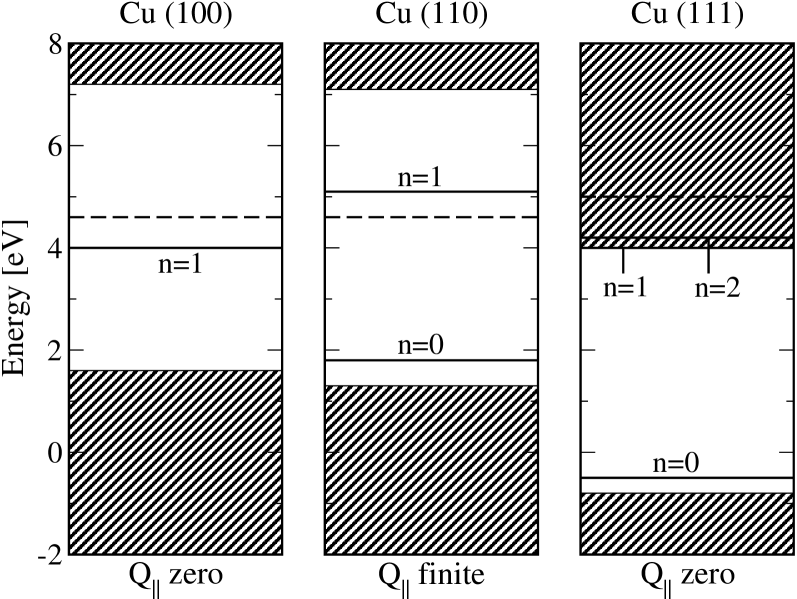
Figure 5: Schematic electronic structure after JDK86 for a copper (100), a copper (110), and a copper (111) surface, respectively, for the lateral momentum where the projected energy gap is largest: $|\vec{Q}|=0$ for Cu (100) and Cu (111); $|\vec{Q}|=1.2\AA^{-1}$ in $[\bar{1}10]$ direction for Cu (110). Shaded areas denote the projected bulk band structure and thick solid lines indicate crystal-induced ($n=0$) and polarization-induced ($n\geq 1$) surface states. The zero of the energy axis is the Fermi energy and the vacuum level is given by the dashed line.

Each facet may give rise to two types of surface states: (i) Crystal-induced surface states due to the abrupt appearance (from the plasma electron’s point of view) of a periodic potential inside the grain and (ii) polarization-induced image states, on which the considerations of the previous section were based. Compared to the binding energy of image states, the binding energy of crystal-induced surface states is very large. Instead of a few tenth of an electron volt, it is typically a few electron volts. As a result, the center of gravity of crystal-induced surface states is much closer to the surface than the center of gravity of image states.

Based on the experimental results of JDK86 we show in Fig. 5 as an example the schematic electronic structure of three copper surfaces, respectively, for the lateral momentum where the projected energy gap is largest. The electronic structure for a given orientation changes with momentum (not shown) but for all orientations, and that is the point we want to make, surface states exist, in addition to projected bulk states, and may thus participate in a physisorption process. For dielectric surfaces the electronic structure is quite similar although the details and physical origin of the states is different Spanjaard96 .

An ab-initio modeling of surface states is complex and computationally expensive, even for planar surfaces (see for instance HFH98 ). Fortunately, the essential physics can be understood within simple one dimensional models which assume the potential energy to vary only normally to the surface ($z-$direction) as illustrated in Fig. 6. Inside the material ($z<0$) the potential has the periodicity of the crystal. It may thus lead to an energy gap on the surface. Outside the material, the potential gives rise to a barrier which merges at large distances with the asymptotics of the image potential $V_{p}(z)\sim-1/z$. Its physical origin are exchange and correlation effects which, on the one hand, contribute to the confinement of electrons inside the material and, on the other hand, cause the attraction of external electrons to the surface. A simple microscopic model for the image potential RM72 ; EM73 is given in appendix A.

The situation shown in Fig. 6 is the most favorable one for physisorption of electrons. The vacuum (plasma) potential, which is the zero of the energy scale, is in the middle of a large energy gap. Four main classes of states can then be distinguished: (i) Volume states periodic inside the material and exponentially decaying into the vacuum (plasma). They exist for energies where bulk states are also allowed. Close to band edges they may have an increased weight near the surface in which case they are surface resonances. (ii) Bound surface states, that is, states decaying exponentially into the material and the vacuum. They appear in regions of negative energies where bulk states are absent: Weakly bound image states close to the vacuum potential and strongly bound crystal-induced surface states close to the Fermi energy. Crystal-induced surface states may have tails on the material side strongly oscillating with the crystal periodicity, while the tails of image states may only weakly respond to the crystal potential. (iii) Unbound surface states for positive energies inside the gap. They are free on the vacuum and bound on the material side. The periodic crystal potential may also not affect these states very much. (iv) States which are free on both sides. Inside the material they oscillate with the lattice periodicity while outside the material their oscillations have to fit the surface potential. In the vicinity of the surface this class of states may also have a peak.

Of particular importance for sticking and desorption are transitions between bound and unbound surface states due to inelastic scattering with elementary excitations of the boundary. The elementary excitations can be phonons, plasmons, and electron-hole pairs. The latter two cases are excitations involving volume states.

The potential plotted in Fig. 6 is for an uncharged surface. An electron approaching a plasma boundary is of course also subject to the Coulomb repulsion due to the electrons already residing on the surface. In the meanfield approximation, however, this repulsion leads only to a barrier whose height is the floating energy $\bar{U}$. Only an electron with an energy larger than $\bar{U}$ has a chance to come close enough to the surface to feel the attractive part of the potential. For an electron bound in this part of the potential, on the other hand, the Coulomb barrier merely sets the ionization threshold. Thus, as long as the Coulomb repulsion is treated in meanfield approximation, the Coulomb term drops out from the considerations provided we shift the zero of the energy axis to $\bar{U}$, that is, by simply measuring energies with respect to the floating energy (Coulomb barrier) of the surface. If $\bar{U}$ falls inside an energy gap of the boundary the situation is similar to the one depicted in Fig. 6.

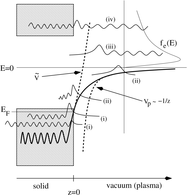
Figure 6: Schematic drawing of the potential energy at a surface (plasma boundary) such as copper (100) or copper (110) and representative wavefunctions for volume states (i), bound surface states (ii), unbound surface states (iii), and free states (iv). Shaded areas denote projected bulk states, $E_{F}$ is the Fermi energy of the solid, $E=0$ is the vacuum (i.e. floating) level, and $f_{e}(E)$ is the plasma electron’s Boltzmann distribution function. The dashed lines indicate the approximate potentials defining the simplified planar model of subsection 3.2 on which the calculation of $s_{e}$ and $\tau_{e}$ is based we describe, respectively, in subsection 3.3 and 3.4.

3.2 Simplified planar microscopic model

Ideally, a microscopic calculation of $s_{e}$ and $\tau_{e}$ for a spherical grain would be based on a three-dimensional first-principle electronic structure of the grain surface.

In view of the discussion of the previous subsection an estimate for the grain’s $s_{e}$ and $\tau_{e}$ may be however also obtained by the following strategy which is most probably simpler because it allows to incorporate existing (one-dimensional) empirical pseudo-potentials for planar surfaces: (i) Identify the facets on the grain surface and neglect, in a first approximation, the finite lateral extension of the facets, that is, work with plane waves or Bloch functions in the lateral dimensions. (ii) Use empirical one-dimensional potentials for planar surfaces CSE99 to calculate for each facet separately bound and unbound surface states. (iii) Identify the channels for electron energy relaxation and set up, again for each facet separately, a quantum-kinetic scheme for the calculation of $s_{e}$ and $\tau_{e}$. (iv) Use an appropriate macroscopic spatial averaging scheme to obtain an estimate for the grain’s $s_{e}$ and $\tau_{e}$.

Despite its approximate nature this strategy is still demanding. To work it out for a realistic grain is surely beyond the scope of this colloquium. In the exploratory calculation of $s_{e}$ and $\tau_{e}$ presented below we focused therefore on a single, infinitely extended facet, that is, on a planar surface, whose electronic structure we moreover did not deduce from an empirical pseudo-potential but from a model potential which is amenable to analytical treatment while at the same time it retains the essential physics.

Quite generally, the probability with which an electron approaching from the plasma halfspace $z>0$ the plasma boundary at $z=0$ ends up in a bound surface state (sticking), or with which an electron bound to the surface ends up in a free state (desorption) can be obtained from a Hamiltonian,

$$H=H_{e}+H_{s}+H_{es}~{},$$ (27)

where the first term describes the electron motion in the static surface potential, the second term denotes the free motion of the elementary excitations of the boundary controlling electron energy relaxation at the boundary and thus physisorption of electrons, and the third term is the coupling between the two.

It is advantageous to express the Hamiltonian (27) in terms of creation and annihilation operators for the (external) electron as well as the (internal) elementary excitations. For that purpose we use the basis in which $H_{e}$ is diagonal, that is, the eigenstates of the static surface potential $V(z)$.  Writing ${\bf r}=({\bf R},z)$ for the electron position, the Schrödinger equation defining these states reads

$$\bigg{(}-\frac{\hbar^{2}}{2m_{e}}\Delta+V(z)\bigg{)}\Psi_{\vec{Q}q}(\vec{R},z)=E_{\vec{Q}q}\Psi_{\vec{Q}q}(\vec{R},z)~{}.$$ (28)

The lateral motion is free and can be separated from the vertical one. Hence,

$$\Psi_{\vec{Q}q}(\vec{R},z)=\frac{1}{\sqrt{A}}\exp[i\vec{Q}\cdot\vec{R}]\psi_{q}(z)~{},$$ (29)

with $A$ the area of the surface, which is eventually made infinitely large, $\vec{Q}=(Q_{x},Q_{y})$ a two-dimensional wavevector characterizing the lateral motion of the electron and $\psi_{q}(z)$ the wavefunction for the vertical motion which satisfies the one-dimensional Schrödinger equation (viz: Eq. (10))

$$\frac{d^{2}}{dz^{2}}\psi_{q}(z)+\frac{2m_{e}}{\hbar^{2}}\bigg{[}E_{q}-V(z)\bigg{]}\psi_{q}(z)=0$$ (30)

with $E_{q}=E_{\vec{Q}q}-\hbar^{2}Q^{2}/2m_{e}$. The quantum number $q$ is an integer $n$ for bound and a wavenumber $k$ for unbound surface states. In this basis,

$$H_{e}=\sum_{\vec{Q}q}E_{\vec{Q}q}C_{\vec{Q}q}^{\dagger}C_{\vec{Q}q}~{},$$ (31)

where $C_{\vec{Q}q}^{\dagger}$ creates an electron in the surface state $\Psi_{\vec{Q}q}$ with energy

$$E_{\vec{Q}q}=\hbar^{2}Q^{2}/2m_{e}+E_{q}~{}.$$ (32)

Table 1: Dielectric constant $\epsilon$, Debye Energy $k_{B}T_{D}$, and the energy separations between the four lowest image states for different materials.

material	$\epsilon$	$k_{B}T_{D}[eV]$	$\Delta E_{21}[eV]$	$\Delta E_{43}[eV]$
Cu	$\infty$	0.03	0.64	0.12
Si	12	0.057	0.46	0.09
graphite	12	0.19	0.46	0.09
$C_{60}$	4.5	0.016	0.26	0.05

The second and third term in (27) depend on the kind of elementary excitations responsible for energy relaxation and hence on the material. For dielectric materials, such as graphite or silicon, the coupling to vibrational modes is most probably the main driving force for physisorption of electrons. In particular, lattice vibrations should play an important role. Their energy scale is the Debye energy $k_{B}T_{D}$. For most dielectrics $k_{B}T_{D}$ is smaller than the energy spacing of the lowest surface states. For image states typical energy separations are given in table 1. When crystal-induced surface states or dangling bonds Spanjaard96 ) are also included the situation does not change much, it may be even worse. Multiphonon processes could thus significantly affect physisorption of electrons at dielectric surfaces making it a very interesting problem to study.

For metals, on the other hand, electronic excitations, most notably electron-hole pairs, provide an efficient channel for electron energy relaxation NNS86 ; WJS92 . They are not created across a large energy gap, as in dielectrics, where they are therefore unimportant, but with respect to the Fermi energy of a partially filled band. In metals electron-hole pairs can be excited even at room temperature. Physisorption of electrons at metallic plasma boundaries, whose temperatures are typically not much higher than room temperature, is thus most likely controlled by the coupling to electron-hole pairs.

The Fermi energy of a metal is inside a band. Electron-hole pairs are thus excitations involving volume states. Ignoring, in a first approximation, exchange between these states and (bound and unbound) surface states, which should be small because the states are spatially separated (see Fig. 6), electrons occupying these two classes of states can be approximately treated as two separate species: External and internal electrons, where the latter are responsible for energy relaxation of the former.

Specifically for a metallic plasma boundary, and we will restrict the calculation of $s_{e}$ and $\tau_{e}$ presented in the next two subsections to this particular case, $H_{s}$ is thus the Hamiltonian of a non-interacting gas of electronic quasi-particles with Fermi energy $E_{F}$. Hence,

$$H_{s}=\sum_{\vec{K}k}E_{\vec{K}k}D_{\vec{K}k}^{\dagger}D_{\vec{K}k}~{},$$ (33)

with $D_{\vec{K}k}^{\dagger}$ creating an internal electron in a quasi-particle state

$$\Phi_{\vec{K}k}(\vec{R},z)=\frac{1}{\sqrt{A}}\exp[i\vec{K}\cdot\vec{R}]\phi_{k}(z)$$ (34)

with energy

$$E_{\vec{K}k}=\frac{\hbar^{2}K^{2}}{2m_{e}}+\tilde{E}_{k}~{}.$$ (35)

In the above expressions we ignored the periodic crystal potential inside the material. It could be taken into account using for the lateral motion Bloch states instead of plane waves and effective electron masses, possibly different for the lateral and vertical motions, instead of the bare electron mass.

Table 2: Fermi energy $E_{F}$, Fermi wavenumber $k_{F}$, and screening wavenumber $(k_{s})_{\rm bulk}$ for various metals AshcroftMermin .

metal	$E_{F}[eV]$	$k_{F}[\AA^{-1}]$	$(k_{s})_{\rm bulk}/k_{F}$
Ag	5.49	1.20	1.42
Cu	7.0	1.36	1.33
Al	11.7	1.75	1.17

The function $\phi_{k}(z)$, describing the vertical motion of an internal electron, obeys a one-dimensional Schrödinger equation:

$$\frac{d^{2}}{dz^{2}}\phi_{k}(z)+\frac{2m_{e}}{\hbar^{2}}\bigg{[}\tilde{E}_{k}-\tilde{V}(z)\bigg{]}\phi_{k}(z)=0~{}.$$ (36)

Strictly speaking, the potential $\tilde{V}(z)=V(z)$. But the spatial parts of the potential determining, respectively, surface and volume states are different. Working conceptually with two separate potentials gives us the flexibility to independently extend the relevant parts of the potential such that the calculation of surface and volume states can be most easily performed while the essential physics is kept (see dashed lines in Fig. 6 and below for the particular form of the approximate potentials).

For a metallic boundary, the interaction part $H_{es}$ of the Hamiltonian (27) describes the interaction between internal and external electrons. Anticipating a statically screened Coulomb interaction,

$$H_{es}=\frac{1}{2}\sum_{\vec{Q}q\vec{Q}^{\prime}q^{\prime}\vec{K}k\vec{K}^{\prime}k^{\prime}}\!\!\!\!V_{\vec{Q}^{\prime}q^{\prime}\vec{K}^{\prime}k^{\prime}}^{\vec{Q}q~{}~{}\vec{K}k}C_{\vec{Q}q}^{\dagger}C_{\vec{Q}^{\prime}q^{\prime}}D_{\vec{K}k}^{\dagger}D_{\vec{K}^{\prime}k^{\prime}}$$ (37)

with

$$V_{\vec{Q}^{\prime}q^{\prime}\vec{K}^{\prime}k^{\prime}}^{\vec{Q}q~{}~{}\vec{K}k} = \frac{2\pi e^{2}}{A^{2}}\frac{\delta(\vec{Q}-\vec{Q}^{\prime}+\vec{K}-\vec{K}^{\prime})}{\sqrt{k_{s}^{2}+(\vec{Q}-\vec{Q}^{\prime})^{2}}}$$ (38)

$$\times I_{q^{\prime}k^{\prime}}^{qk}(\vec{Q}-\vec{Q}^{\prime})$$

and

$$I_{q^{\prime}k^{\prime}}^{qk}(\vec{Q})\!=\!\!\int\!\!\!dzdz^{\prime}\!\psi^{*}_{q}(z)\phi^{*}_{k}(z^{\prime})e^{-d|z-z^{\prime}|}\phi_{k^{\prime}}(z^{\prime})\psi_{q}(z)~{}\!\!,$$ (39)

where $d=\sqrt{k_{s}^{2}+\vec{Q}^{2}}$ and $k_{s}=(k_{s})_{\rm surface}$ is the screening wavenumber at the surface. Little is known about this parameter except that it should be less then the bulk screening wavenumber $(k_{s})_{\rm bulk}$ because the electron density in the vicinity of the boundary is certainly smaller than in the bulk. In NNS86 it was for instance argued, based on a comparison of experimentally and theoretically obtained branching ratios for positron trapping at and transmission through various metallic films that $(k_{s})_{\rm surface}\simeq 0.6(k_{s})_{\rm bulk}$. Bulk screening wavenumbers for some metals are given in table 2.

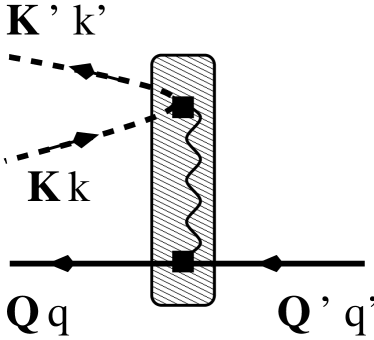
Figure 7: Diagrammatic representation of the golden rule (40) for a transition from the surface state $(\vec{Q}^{\prime}q^{\prime})$ to the surface state $(\vec{Q}q)$ (solid lines) via scattering on an internal electron (dashed line) which can be interpreted as the coupling to internal electron-hole pairs. The wavy line denotes the screened Coulomb interaction between internal and external electrons and the box symbolizes the dynamic, that is, inelastic electron-metal interaction.

The Hamiltonian (27) with $H_{e}$, $H_{s}$, and $H_{es}$ respectively given by (31), (33), and (37) can be used to calculate the transition rate from any initial surface state $\psi_{\vec{Q}^{\prime}q^{\prime}}$ to any final surface state $\psi_{\vec{Q}q}$. For the sticking process the initial state belongs to the continuum of surface states and the final state is a bound surface state while for the desorption process it is vice versa. In lowest order perturbation theory (see Fig. 7), the rate is given by the golden rule,

$${\cal W}(\vec{Q}q,\vec{Q}^{\prime}q^{\prime}) = \frac{2\pi}{\hbar}\sum_{\vec{K}\vec{K}^{\prime}}\sum_{kk^{\prime}}\big{|}V_{\vec{Q}^{\prime}q^{\prime}\vec{K}^{\prime}k^{\prime}}^{\vec{Q}q~{}~{}\vec{K}k}\big{|}^{2}$$ (40)

$$\times n_{F}(E_{\vec{K}^{\prime}k^{\prime}})[1-n_{F}(E_{\vec{K}k})]$$

$$\times \delta(E_{\vec{Q}^{\prime}q^{\prime}}+E_{\vec{K}^{\prime}k^{\prime}}-E_{\vec{Q}q}-E_{\vec{K}k})~{},$$

where $n_{F}(E)=1/(\exp[(E-E_{F})/k_{B}T_{s}]+1)$ is the Fermi distribution function for the metal electrons with Fermi energy $E_{F}$ and temperature $T_{s}$.

To calculate the matrix element (39) we need the solutions of the Schrödinger equations (30) and (36). Physisorption of electrons involves transitions between bound and unbound surface states. The matrix elements for these transitions are large when the spatial overlap between the initial and final states is large. With unbound surface states inside the gap, image states, that is, bound surface states close to the zero of the energy axis (see Fig. 6), have the largest overlap. Crystal-induced surface states, having most weight in regions where the weight of unbound surface states is very small, give rise to a smaller overlap and are thus less important. We neglect therefore crystal-induced surface states and replace $V(z)$ in (30) by

$$V(z)\rightarrow\left\{\begin{array}[]{ll}\infty&\mbox{for}~{}z\leq 0\\ V_{p}(z)&\mbox{for}~{}z>0~{},\end{array}\right.$$ (43)

where

$$V_{p}(z)=-\frac{e^{2}}{4z}$$ (44)

is the classical image potential. As explained in appendix A, $V_{p}$ can be understood in terms of virtual surface plasmon excitations RM72 ; EM73 ; Barton81 . We thus calculated the surface states as if the energy gap on the surface were infinitely large. The solutions of (30) are then Whittaker functions which vanish for $z\leq 0$ (see Appendix B) and the required matrix elements can be obtained analytically.

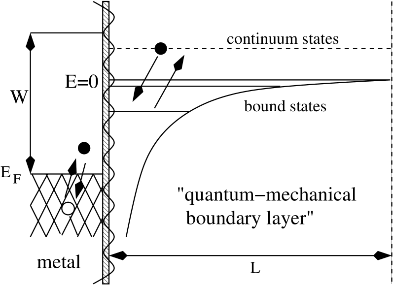
Figure 8: Illustration of the microphysics for a plasma electron approaching a metallic boundary. The wavy line indicates the surface mode responsible for the attractive polarization potential (“image potential”) and $L$ is the width of the “boundary layer” where a quantum-mechanical calculation applies. The electron looses (gains) energy due creation (annihilation) of electron-hole pairs in the metal. Due to these processes it may get trapped in (escape from) the bound states of the polarization potential. In other words, it may get stuck at (desorb from) the plasma boundary. $W$ and $E_{F}$ are, respectively, the work function and the Fermi energy of the metal.

As far as volume states required for the construction of internal electron-hole pairs are concerned, we followed NNS86 ; WJS92 and calculated these states as if the work function $W$ of the metal where infinite. Measuring moreover energies inside the material from the average of the crystal potential and neglecting the oscillations of the potential, that is, treating the metal boundary as a jellium halfspace,

$$\tilde{V}(z)\rightarrow\left\{\begin{array}[]{ll}0&\mbox{for}~{}z<0\\ \infty&\mbox{for}~{}z\geq 0~{}.\end{array}\right.$$ (47)

The wavefunctions $\phi_{k}(z)$ vanish then for $z\geq 0$ and are standing waves for $z<0$. Using box-normalization,

$$\phi_{k}(z)=\sqrt{\frac{2}{L}}\sin(kz)$$ (48)

leading to $\tilde{E}_{k}=\hbar^{2}k^{2}/2m_{e}$ with $k=\pi n/L$ and $n\geq 1$ an integer. In the final expressions for $s_{e}$ and $\tau_{e}$ we use $L\rightarrow\infty$ making $k$ continuous.

The physical content of the simplified planar model is summarized in Fig. 8. It will be used in the next two subsections to calculate, respectively, $s_{e}$ and $\tau_{e}$ for a metallic plasma boundary. Due to the approximate potentials (43) and (47), external and internal single electron wavefunctions vanish in complementary halfspaces. As a result, the matrix element (39) factorizes,

$$I_{q^{\prime}k^{\prime}}^{qk}(\vec{Q})=I_{qq^{\prime}}^{(1)}(\vec{Q})I_{kk^{\prime}}^{(2)}(\vec{Q})$$ (49)

with

$$I_{qq^{\prime}}^{(1)}(\vec{Q})\!\! = \!\!\int_{0}^{\infty}\!\!\!dz\exp[-z\sqrt{k_{s}^{2}+\vec{Q}^{2}}]\psi_{q}^{*}(z)\psi_{q^{\prime}}(z)~{},$$ (50)

$$I_{kk^{\prime}}^{(2)}(\vec{Q})\!\! = \!\!\int_{0}^{\infty}\!\!\!dz\exp[-z\sqrt{k_{s}^{2}+\vec{Q}^{2}}]\phi_{k}^{*}(-z)\phi_{k^{\prime}}(-z)~{}$$ (51)

to be calculated explicitly in appendix B.

A rigorous calculation of $s_{e}$ and $\tau_{e}$, taking for instance into account that sticking and desorption occur on different timescales Brenig82 , should be based on quantum-kinetic master equations for the time-dependent occupancies of the surface states $\psi_{\vec{Q}q}$. The master equations could be derived from (27) with techniques from non-equilibrium physics KG86 . In lowest order perturbation theory, the transition rates appearing in the master equation would be given by (40). In the following, we will not use this advanced approach. Instead we will calculate $s_{e}$ and $\tau_{e}$ perturbatively by appropriately summing and weighting the transition rate (40) over initial and final states.

3.3 Sticking coefficient

In order to calculate the sticking coefficient $s_{e}$ we consider the positive half space ($z>0$) as a kind of quantum-mechanical boundary layer (see Fig. 8). A measure of the tendency $S_{\vec{Q}n,\vec{Q}^{\prime}q^{\prime}}$ with which an electron approaching in an unbound state $\Psi_{\vec{Q}^{\prime}q^{\prime}}$ the plasma-boundary at $z=0$ gets stuck in a bound state $\Psi_{\vec{Q}n}$ is then the time it takes the electron to traverse the boundary layer forwards and backwards divided by the time it takes the electron to make a transition from $\Psi_{\vec{Q}^{\prime}q^{\prime}}$ to $\Psi_{\vec{Q}n}$ GS91 .

Since the width of the quantum-mechanical boundary layer is $L$,

$$S_{\vec{Q}n,\vec{Q}^{\prime}q^{\prime}}=\frac{2L}{{}_{\rm in}\langle\vec{Q}^{\prime}q^{\prime}|\frac{\vec{p}\cdot\vec{n}}{m_{e}}|\vec{Q}^{\prime}q^{\prime}\rangle_{\rm in}}\times\frac{1}{{\cal W}^{-1}(\vec{Q}n,\vec{Q}^{\prime}q^{\prime})}~{},$$ (52)

where the denominator in the first factor is the velocity matrix element calculated with the incoming part of the state $\Psi_{\vec{Q}^{\prime}q^{\prime}}$; $\vec{n}$ is the normal vector of the boundary pointing towards the plasma and $\vec{p}=-i\hbar\nabla$, the quantum-mechanical momentum operator. Using the asymptotic form of the unbounded wavefunctions given in Eq. (91) of appendix B, we find

$${}_{\rm in}\langle\vec{Q}^{\prime}q^{\prime}|\frac{\vec{p}\cdot\vec{n}}{m_{e}}|\vec{Q}^{\prime}q^{\prime}\rangle_{\rm in}=\frac{\hbar q^{\prime}}{8m_{e}a_{B}}~{}.$$ (53)

Hence,

$$S_{\vec{Q}n,\vec{Q}^{\prime}q^{\prime}}=\frac{16Lm_{e}a_{B}}{\hbar q^{\prime}}{\cal W}(\vec{Q}n,\vec{Q}^{\prime}q^{\prime})~{}.$$ (54)

The tendency with which the electron approaching the boundary in the state $\Psi_{\vec{Q}^{\prime}q^{\prime}}$ gets stuck in any one of the bound states – the energy resolved sticking coefficient – is then simply given by

$$S_{\vec{Q}^{\prime}q^{\prime}} = \sum_{\vec{Q}n}S_{\vec{Q}n,\vec{Q}^{\prime}q^{\prime}}$$ (55)

$$= \frac{16Lm_{e}a_{B}}{\hbar q^{\prime}}\sum_{n\vec{Q}}{\cal W}(\vec{Q}n,\vec{Q}^{\prime}q^{\prime})~{}.$$

The sticking coefficient $s_{e}$ entering the rate equation (2) is an energy-averaged sticking coefficient resulting from an appropriately performed sum over $S_{\vec{Q}^{\prime}q^{\prime}}$. As mentioned before, a rigorous derivation of an expression for $s_{e}$ should be based on the master equation for the occupancies of the surface states Brenig82 ; KG86 . A simpler way to obtain $s_{e}$ is however to regard the wall as a particle detector. The global sticking coefficient can then be defined as

$$\sum_{\vec{Q}^{\prime}q^{\prime}}S_{\vec{Q}^{\prime}q^{\prime}}q^{\prime}n_{\vec{Q}^{\prime}q^{\prime}}=s_{e}\sum_{\vec{Q}^{\prime}q^{\prime}}q^{\prime}n_{\vec{Q}^{\prime}q^{\prime}}~{},$$ (56)

where $n_{\vec{Q}^{\prime}q^{\prime}}$ are the occupancies of the unbound surface states $\Psi_{\vec{Q}^{\prime}q^{\prime}}$.

The occupancies $n_{\vec{Q}^{\prime}q^{\prime}}$ depend on the properties of the plasma. It is tempting to simply identify $n_{\vec{Q}^{\prime}q^{\prime}}$ with the incoming part of the electron distribution function as it arises on the surface from the solution of the Boltzmann-Poisson equations. However, one should keep in mind that the distribution function is a classical object whereas $n_{\vec{Q}^{\prime}q^{\prime}}$ is a quantum-mechanical expectation value. There arises therefore the question how the quantum-mechanical processes encoded in the above equations can be properly fed into the semiclassical description of the plasma in terms of Boltzmann-Poisson equations. The issue is subtle because at the plasma boundary the potential varies so rapidly that the basic assumptions of the validity of the Boltzmann equation no longer hold. Mathematically, the microphysics should be put into a surface scattering kernel, course-grained over a few $nm$, which connects, generally retarded in time, the incoming electron distribution function with the outgoing one. But even for neutral particles, a microscopic derivation of such a scattering kernel has not yet been given. There exist only more or less plausible phenomenological expressions which parameterize the kernel with accommodation coefficients Kuscer71 .

From the boundary-layer point of view used in the derivation of Eqs. (52)–(56), the plasma, or, more precisely, the sheath of the plasma, is infinitely far away from the plasma boundary. Rigorously speaking, we can thus say nothing about how the microphysics at the plasma boundary merges with the physics in the plasma sheath.

To make nevertheless contact with the plasma we have to guess how the unbound surface states $\Psi_{\vec{Q}^{\prime}q^{\prime}}$ are occupied. For simplicity we assume Maxwellian occupancy, with an electron temperature $T_{e}=(k_{B}\beta_{e})^{-1}$, but other guesses, more appropriate for the plasma sheath, are also conceivable. For Maxwellian electrons, the global sticking coefficient is given by

$$s_{e}=\frac{\sum_{\vec{Q}^{\prime}q^{\prime}}S_{\vec{Q}^{\prime}q^{\prime}}q^{\prime}\exp[-\beta_{e}E_{\vec{Q}^{\prime}q^{\prime}}]}{\sum_{\vec{Q}^{\prime}q^{\prime}}q^{\prime}\exp[-\beta_{e}E_{\vec{Q}^{\prime}q^{\prime}}]}~{}.$$ (57)

In the limit $L\rightarrow\infty$ and $A\rightarrow\infty$ the momentum summations in Eqs. (52)–(57) become integrals. The calculation of $S_{\vec{Q}^{\prime}q^{\prime}}$ and $s_{e}$ reduces therefore to the calculation of high-dimensional integrals. In appendix C we describe the approximations invoked for the integrals. Some of the integrals can then be analytically performed. But the final expressions for the sticking coefficients remain multi-dimensional integrals, which have to be done numerically.

Measuring energies in units of $R_{0}$ and distances in units of $a_{B}$, Eq. (57) for the global sticking coefficient reduces to

$$s_{e}=\bigg{(}\frac{4}{\pi}\bigg{)}^{2}\frac{\beta_{e}^{3/2}}{\beta_{s}^{1/2}}I_{\rm stick}~{},$$ (58)

where

$$I_{\rm stick}=\int_{0}^{\infty}\!\!\!dR\int_{-\infty}^{\infty}\!\!\!d\omega\frac{1+n_{B}(\omega)}{1+(R/k_{s})^{2}}h(R,\omega)g(R,\omega)$$ (59)

with $n_{B}(E)=1/(\exp[\beta_{s}E]-1)$ the Bose distribution function and $h(R,\omega)$ and $g(R,\omega)$ two functions defined, respectively, in appendix C by Eq. (110) and (111).

Figure 9: Energy resolved sticking coefficient for an electron hitting perpendicularly an aluminum surface at $k_{B}T_{s}=0.05eV$. The screening wavenumber for the Coulomb interaction between an incident plasma electron and an internal aluminum electron, $(k_{s})_{\rm surface}$, is not well known. Results are therefore shown for $(k_{s})_{\rm surface}/(k_{s})_{\rm bulk}=0.1$ (weak screening, strong coupling) and for $(k_{s})_{\rm surface}/(k_{s})_{\rm bulk}=0.6$ (moderate screening, weak coupling); $(k_{s})_{\rm bulk}$ is the screening wavenumber of aluminum (see table 2). Since $(k_{s})_{\rm surface}=0.6(k_{s})_{\rm bulk}$ is most probably the relevant screening parameter NNS86 ; WJS92 , the sticking coefficient is rather small.

Below we also present results for the energy resolved sticking coefficient for perpendicular incidence $(\vec{Q}^{\prime}=0)$. It is given by

$$S^{\perp}_{E^{\prime}}=\bigg{(}\frac{4}{\pi}\bigg{)}^{2}\!\frac{\pi^{1/2}}{\beta_{s}^{1/2}}\int_{0}^{\infty}\!\!\!\!dRg^{\perp}(R,E^{\prime})~{},$$ (60)

with $E^{\prime}=q^{\prime 2}$ and $g^{\perp}(R,E^{\prime})$ a function defined in appendix C, Eq. (113).

The functions $h(R,\omega)$, $g(R,\omega)$, and $g^{\perp}(R,E^{\prime})$ contain summations over the Rydberg series of bound surface states. If not stated otherwise, we truncated these sums after $N=15$ terms. These functions are moreover defined in terms of integrals which can be done only numerically. We use Gaussian integration with $40-80$ integration points. More specifically, $h(R,\omega)$ and $g^{\perp}(R,E^{\prime})$ are one-dimensional integrals while $g(R,\omega)$ is a two-dimensional one. Hence, $s_{e}$ and $S^{\perp}_{E^{\prime}}$ are given by a five-dimensional and a two-dimensional integral, respectively.

Figure 10: Dependence of the energy resolved sticking coefficient for perpendicular incidence on the number $N$ of bound states included in the calculation. Except of the screening wavenumber, which is set to $(k_{s})_{\rm surface}=0.6(k_{s})_{\rm bulk}$, the parameters are identical to the ones used in Fig. 9. The dashed lines are for $N=10$ and $N=20$, respectively, indicating the fast converge with respect to $N$.

In the formulae for the sticking coefficients we multiplied the binding energies of the surface states $|E_{n}|$ obtained from Eq. (30) by an overall factor of $0.7$. This value was chosen to bring the binding energy of the lowest surface state $|E_{1}|=0.85eV$ in accordance with the experimentally measured value for copper: $|E_{1}|^{\rm Cu}\approx 0.6eV$ EL95 . For other metals we used the same correction factor.

Figure 9 shows the results for $S^{\perp}_{E^{\prime}}$ when an electron with energy $E^{\prime}$ hits perpendicularly an aluminum boundary at $k_{B}T_{s}=0.05eV$. Representative for weak and moderate screening we plotted data for $(k_{s})_{\rm surface}/(k_{s})_{\rm bulk}=0.1$ and $(k_{s})_{\rm surface}/(k_{s})_{\rm bulk}=0.6$. The latter is the screening parameter used in NNS86 ; WJS92 to study the interaction of positrons with an aluminum surface. If the corresponding value for $1/(k_{s})_{\rm surface}$ is indeed a reasonable estimate for the length on which the Coulomb interaction between an external and an internal electron is screened, the sticking coefficient for electrons should be extremely small, of the order of $10^{-4}$. Only for weak screening, and thus strong coupling, does $S^{\perp}_{E^{\prime}}$ approach values of the order of $10^{-1}$ which are perhaps closer to the value one would expect on first sight.

To clarify the contribution the various bound states have to the sticking coefficient, we plot in Fig. 10 the dependence of $S_{E^{\prime}}^{\perp}$ on the number $N$ of bound states included in the calculation. As can be seen, the lowest bound state ($N=1$) contributes only roughly $40\%$ to the total $S_{E^{\prime}}^{\perp}$. The sticking coefficient increases then with increasing $N$ but converges for $N\approx 10-20$. Because of this fast convergence we present all results below only for $N=15$. The reason for the convergence can be traced back to the decrease of the electronic matrix element $I^{(1)}_{kn}(\vec{Q})$ defined in Eq. (50), which we approximate by $I^{(1)}_{k\ll 1n}(\vec{Q}=0)$ (see appendix C), with increasing $n$, where $n=1,2,...$ labels the bound surface states.

Global sticking coefficients $s_{e}$ as a function of the screening wavenumber $(k_{s})_{\rm surface}$ are shown in Fig. 11 for different metals. For $(k_{s})_{\rm surface}/(k_{s})_{\rm bulk}>0.4$, the sticking coefficients are again extremely small. As expected they increase with decreasing $(k_{s})_{\rm surface}/(k_{s})_{\rm bulk}$, reaching values close to unity for weak screening. In this strong coupling regime, our perturbative calculation of $s_{e}$ is no longer valid. We believe however that $(k_{s})_{\rm surface}/(k_{s})_{\rm bulk}<0.4$ is unphysical. The kink around $(k_{s})_{\rm surface}/(k_{s})_{\rm bulk}\approx 0.25$ must be due to an accidental resonance in $g(R,\omega)$. It is of no physical significance.

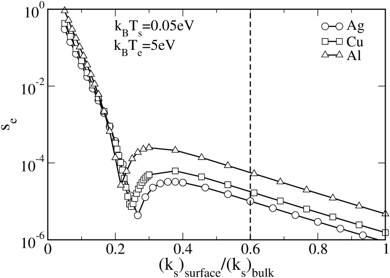
Figure 11: The global sticking coefficient $s_{e}$ for a thermal beam of electrons with $k_{B}T_{e}=5eV$ hitting various metal surfaces at $k_{B}T_{s}=0.05eV$ as a function of $(k_{s})_{\rm surface}/(k_{s})_{\rm bulk}$, where $(k_{s})_{\rm bulk}$ is the screening wavenumber in the bulk of the respective metal (see table 2). Following NNS86 ; WJS92 , we would expect $(k_{s})_{\rm surface}=0.6(k_{s})_{\rm bulk}$ to be a reasonable estimate for the screening parameter. Hence, $s_{e}\approx 10^{-5}-10^{-4}$.

Why is the sticking coefficient for electrons so small? We have no satisfying explanation. Our calculation produces small a sticking coefficient because the matrix element (39) turns out to be very small. We certainly underestimate it because the wavefunctions of the approximate potentials (43) and 47) vanish in complementary halfspaces, in contrast to the exact wavefunctions which have tails. Nevertheless it is hard to image the tails of the wavefunctions to increase the matrix elements by three orders of magnitude.

The approximations we had to make to end up with manageable equations for $s_{e}$, in particular, the assumptions about the momentum dependence of the electronic matrix elements (see appendix C and, for a discussion, the next section) should also not lead to a sticking coefficient which is more than one order of magnitude off. In this respect let us emphasize that in contrast to the calculations performed in NNS86 ; WJS92 for a positron, which produce positron sticking coefficients of the order of $0.1$, we use the eigenenergies and eigenstates of the $1/z$ potential and not the ones of an artificial box potential.

Usually it is assumed that $s_{e}$ is also at least of the order of $0.1$ DS87 . This expectation seems to be primarily based on the semiclassical back-on-the envelop-estimate of Umebayashi and Nakano UN80 . It is thus appropriate to discuss their approach in some detail.

From the energy $\Delta E_{s}$ an electron can exchange in a single classical collision with the constituents of the solid they first estimated, using the analogy to the Mössbauer effect, the probability $\alpha$ for inelastic one-phonon emission. For that purpose, they had to estimate the number $N_{c}$ of constituents of the surface an electron with a de-Broglie wavelength corresponding to its kinetic energy $E_{0}$, $\lambda_{e}^{dB}=2\pi a_{B}\sqrt{R_{0}/E_{0}}$, simultaneously impacts. A rough estimate is $N_{c}=(\lambda_{e}^{dB}/a)^{2}$, where $a$ is the lattice constant of the material. Under the assumption that the electron hops along the surface they then calculated the probability with which the electron does not escape after $l$ hops where $l$ is the number of inelastic collisions which are necessary for the electron to transfer its whole positive kinetic energy to the lattice, that is, to end up in a state of negative energy. Identifying this probability with the (global) sticking coefficient, they obtained

$$s_{e}=\prod_{i=0}^{l-1}\frac{1}{1+\beta_{i}/\alpha}~{},$$ (61)

where $\beta_{i}=(E_{0}-i\Delta E)/E_{b}$ is the escape probability after $i$ inelastic collisions HS70 , $\Delta E=2\Delta E_{s}/3N_{c}\alpha$, $\Delta E_{s}=4m_{e}(E_{0}+E_{b})/M$, $E_{b}$ is the depth of the surface potential and $M$ is the mass of the constituents of the solid.

Sticking coefficients for graphite obtained from Eq. (61) are shown in Fig. 12. Within Umebayashi and Nakano’s semiclassical approach we identified $E_{b}$ with the binding energy of the electron. According to Fig. 12 the sticking coefficient very quickly approaches extremely small values with increasing energy $E_{0}$. The smaller the binding energy $E_{b}$, the faster the decrease. The values for $s_{e}$ originally given by Umebayashi and Nakano were for kinetic energies smaller than $0.0026eV$ and binding energies larger than $1eV$. Only in this parameter regime is the sticking coefficient close to one. In the parameter range which is of interest to us (kinetic and binding energies at least a few tenth of an electron volt) Umebayashi and Nakano’s estimate gives also an extremely small sticking coefficient.

Figure 12: Electron sticking coefficient obtained from Umebayashi and Nakano’s phenomenological model UN80 , see Eq. (61). The solid lines are for the $e^{-}$:graphite system originally considered by them ($k_{B}T_{D}=420K$, $M_{\rm C}=12m_{p}$, where $m_{p}$ is the proton mass, and $a=2.5\AA$) and the dashed line is for an $e^{-}$:Cu system ($E_{b}=0.6eV$, $k_{B}T_{D}=343K$, $M_{\rm Cu}=64m_{p}$, and $a=3.61\AA$). The sticking coefficient diminishes rapidly with increasing electron energy and approaches one at zero electron energy, in contrast to what one would expect from a quantum-mechanical calculation BR92 .

We should of course not directly compare the results obtained from Eq. (58) with the ones obtained from Eq. (61) because Eq. (58) assumes energy relaxation due to internal electron-hole pairs whereas Eq. (61) assumes energy relaxation due to phonons. However, a quantum-mechanical calculation of the phonon-induced electron sticking coefficient at vanishing lattice temperature also shows that $s_{e}\approx 10^{-4}$ BR92 , in contrast to what Umebayashi and Nakano find. Although they incorporate some quantum mechanics their approach is basically classical. It is based on the notion of a classical particle hopping around on the surface and exchanging energy with the solid in binary encounters. As in any classical theory for the sticking coefficient, it is therefore not surprising that the sticking coefficient they obtain approaches unity for the low energies they consider KG86 .

3.4 Desorption time

We now calculate the electron desorption time $\tau_{e}$. For that purpose, we have to specify the occupancies of the bound electron surface states. In general, this is a critical issue. However, provided the desorption time $\tau_{e}$ is much larger than the time it takes to establish thermal equilibrium with the boundary, it is plausible to assume that bound electron surface states are populated according to

$$n_{\vec{Q}n}\sim\exp[-\beta_{s}E_{\vec{Q}n}]~{},$$ (62)

where $T_{s}=1/k_{B}\beta_{s}$ is the surface temperature.

Desorption is accomplished as soon as the electron is in any one of the unbound surface states. Hence, the inverse of the desorption time, that is, the desorption rate, is given by KG86

$$\frac{1}{\tau_{e}}=\frac{\sum_{\vec{Q}^{\prime}n^{\prime}}\sum_{\vec{Q}q}\exp[-\beta_{s}E_{\vec{Q}^{\prime}n^{\prime}}]{\cal W}(\vec{Q}q,\vec{Q}^{\prime}n^{\prime})}{\sum_{\vec{Q}n}\exp[-\beta_{s}E_{\vec{Q}n}]}~{},$$ (63)

where ${\cal W}(\vec{Q}q,\vec{Q}^{\prime}n^{\prime})$ is the transition rate from the bound surface state $(\vec{Q}^{\prime},n^{\prime})$ to the unbound surface state $(\vec{Q},q)$ as defined by the golden rule (40).

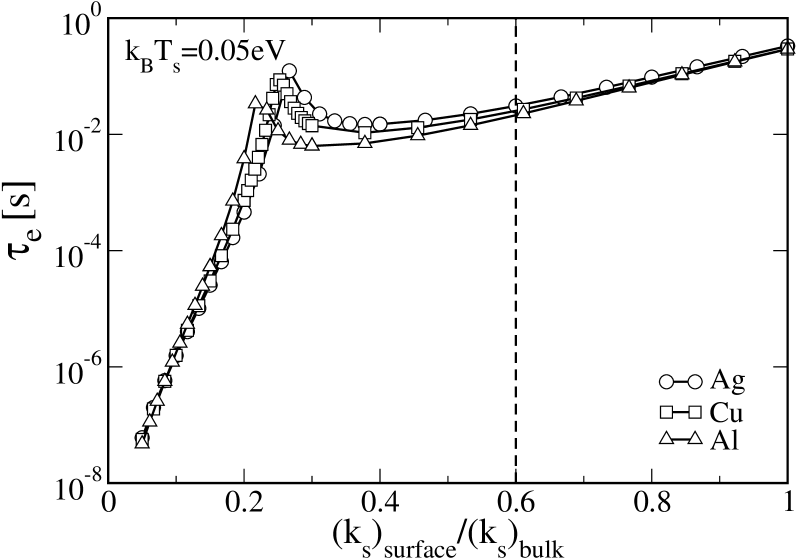
Figure 13: Desorption time $\tau_{e}$ for an electron bound in the polarization-induced external surface states of various metal surfaces at $k_{B}T_{s}=0.05eV$ as a function of $(k_{s})_{\rm surface}/(k_{s})_{\rm bulk}$. Since $(k_{s})_{\rm surface}=0.6(k_{s})_{\rm bulk}$ is most probably the relevant screening wavenumber NNS86 ; WJS92 , $\tau_{e}\approx 10^{-2}s$. For the used material parameters, see table 2.

Measuring again energies in units of $R_{0}$ and distances in units of $a_{B}$ and using the same approximations as in the calculation of the sticking coefficient (see appendix C) the desorption rate can be cast into

$$\tau_{e}^{-1}=\frac{R_{0}}{2\pi^{3}\hbar Z}I_{\rm desorb}~{},$$ (64)

where

$$I_{\rm desorb} = \int_{0}^{\infty}\!\!\!\!dR\!\int_{-\infty}^{\infty}\!\!\!\!\!d\omega\frac{1+n_{B}(\omega)}{1+(R/k_{s})^{2}}f(R,\omega)g(R,\omega)~{},$$ (65)

$Z=\sum_{n}\exp[-\beta_{s}E_{n}]$, $n_{B}(E)$ is again the Bose distribution function, and $f(R,\omega)$ is an one-dimensional integral defined in appendix C, Eq. (117). Thus, to obtain $\tau_{e}^{-1}$ from Eq. (64) we have to do a five-dimensional integral. As for the calculation of $s_{e}$ we again use Gaussian quadratures for that purpose.

In Figure 13 we present, as a function of the screening parameter, numerical results for $\tau_{e}$ for an electron bound in the polarization-induced external surface states of various metal surfaces at $k_{B}T_{s}=0.05eV$. To be close to reality, we again corrected the binding energies $|E_{n}|$ by a factor $0.7$. As can be seen, except for small screening parameters and thus strong coupling, $\tau_{e}\approx 10^{-2}s$.

Compared to typical desorption times for neutral mole- cules, which are of the order of $10^{-6}s$ or less KG86 , the electron desorption time we find is rather long. This is a consequence of our assumption that the bound electron is in thermal equilibrium with the surface (viz: Eq. (62)) and the fact that the binding energy of the lowest surface state $|E_{1}|\gg k_{B}T_{s}$. Thus, the electron desorbs de facto from the lowest surface state which has a binding energy of $\sim 0.6eV$. The binding energies for neutral molecules, on the other hand, are typically one order smaller and thus of the order of $k_{B}T_{s}$ resulting in much larger desorption rates and thus shorter desorption times.

In the model for the quasi-stationary charge of a dust particle presented in the previous section the product $(s\tau)_{e}$ was of central importance. Combining (58) and (64), the microscopic approach gives

$$(s\tau)_{e}=\frac{h}{(k_{B}T_{e})^{3/2}(k_{B}T_{s})^{-1/2}}\frac{16I_{\rm stick}}{I_{\rm desorb}}\sum_{n}\exp[\beta_{s}|E_{n}|]~{},$$ (66)

where $I_{\rm stick}$ and $I_{\rm desorb}$ are defined in Eqs. (59) and (65), respectively.

Figure 14: The product $s_{e}\tau_{e}$ as a function of $k_{B}T_{e}$ for a thermal beam of electrons hitting a copper surface at various temperatures $k_{B}T_{s}$. The surface screening wavenumber is set to $(k_{s})_{\rm surface}=0.6(k_{s})_{\rm bulk}$, where $(k_{s})_{\rm bulk}$ is the screening wavenumber for copper (see table 2).

Figure 14 shows numerical results for $(s\tau)_{e}$ for a copper surface as a function of the electron and surface temperature. The screening wavenumber $(k_{s})_{\rm surface}=0.6(k_{s})_{\rm bulk}$ and the binding energies are again corrected by the factor $0.7$ which makes $|E_{1}|$ to coincide with the experimental value for copper. Notice, the weak dependence of the product $(s\tau)_{e}$ on the electron temperature and the rather strong dependence on the surface temperature. The latter is of course a consequence of the exponential function in Eq. (66). Although the sticking coefficient and desorption times have values which are perhaps in contradiction to naive expectations, $s_{e}$ being extremely small and $\tau_{e}$ being rather large, the product $(s\tau)_{e}$ has the order of magnitude expected from our surface model (see section 2). In particular, $(s\tau)_{e}\simeq 10^{-6}s$ for $k_{B}T_{s}=0.045eV$ would produce grain charges of the correct order of magnitude. Thus, using Eq. (66) instead of Eq. (15) and $k_{B}T_{s}$ as an adjustable parameter, which is still necessary because the grain temperature is unknown, we could produce, for physically realistic surface temperatures, surface charges for metallic grains which are in accordance with experiment WHR95 .

Although the microscopic Eq. (66) has a similar structure as the phenomenological expression (15) there are significant differences. First, the microscopic formula contains more than one bound state and depends not only on $T_{s}$ but also on $T_{e}$. In addition, there is a numerical factor $16=2\times 8$ where the factor $2$ comes from the fact that an electron traversing the quantum-mechanical boundary layer can make a transition to a bound state on its way towards the surface and on its way back to the plasma and the factor $8$ originates from the asymptotic form of the wavefunction for the incoming electron. The phenomenological approach simply assumes here a plane wave whereas the microscopic approach works with Whittaker functions (see appendix B and C). Most importantly, however, the two functions $I_{\rm stick}$ and $I_{\rm desorb}$, which depend on the microscopic details of the inelastic scattering process driving physisorption, and thus on the electron and surface temperature as well as material parameters such as the screening wavenumber, are in general not identical. Hence, $I_{\rm stick}/I_{\rm desorb}\neq 1$.

For the hypothetical case of a single bound state, however, whose binding energy $|E_{1}|$ is much larger than $k_{B}T_{s}$ and $k_{B}T_{e}$, Eq. (66) reduces to a form which, for $k_{B}T_{e}=k_{B}T_{s}$, becomes identical to the phenomenological expression (15), except of the numerical factor referred to in the previous paragraph. The simplification arises because for low temperatures the integrals defining $I_{\rm stick}$ and $I_{\rm desorb}$ can be calculated asymptotically within Laplace’s approximation (see appendix C). The sticking coefficient and desorption time are then given by

$$s^{L}_{e} = \frac{4\big{|}I_{1}^{(1)}\big{|}^{2}\bar{g}}{\pi\beta^{1/2}_{s}\beta^{1/2}_{e}}~{},$$ (67)

$$\tau^{L}_{e} = 8\pi^{2}\beta_{s}^{2}\frac{\hbar}{R_{0}}\frac{\exp[\beta_{s}|E_{1}|]}{\big{|}I^{(1)}_{1}\big{|}^{2}\bar{g}}~{},$$ (68)

with $\bar{g}$ defined in appendix C, Eq. (124). Thus, the product,

$$(s\tau)_{e}^{L}=\frac{16h}{(k_{B}T_{s})^{3/2}(k_{B}T_{e})^{-1/2}}\exp[\beta_{s}|E_{1}|]~{},$$ (69)

is independent of the microscopic details of the inelastic scattering processes encoded in the product $|I^{(1)}_{1}|^{2}\bar{g}$. Identifying $|E_{1}|$ with the electron desorption energy $E_{e}^{d}$ and setting $k_{B}T_{e}=k_{B}T_{s}$, we finally obtain, except of the numerical factor $16=8\times 2$, from Eq. (69) the phenomenological expression (15).

Using Eqs. (67)–(69) we find for an electron at a copper boundary with $k_{B}T_{e}=k_{B}T_{s}=0.045eV$, $s_{e}^{L}=6.23\times 10^{-6}$, $\tau_{e}^{L}=0.131s$, and $(s\tau)_{e}^{L}=8.17\times 10^{-7}s$. Taking only one bound state into account, the corresponding values obtained from Eqs. (58) and  (64) are $s_{e}=4.42\times 10^{-6}$ and $\tau_{e}=0.135s$, which leads to $(s\tau)_{e}=6\times 10^{-7}s$, indicating that at low temperatures Laplace’s approximation works indeed reasonably well. Since $\tau_{e}$ does not depend on $k_{B}T_{e}$ and $k_{B}T_{s}$ is usually much smaller than $|E_{1}|$, approximation (68) for $\tau_{e}$ can be actually always applied, provided the assumption is correct, that the electron is initially in thermal equilibrium with the surface and hence basically in its lowest bound state. The approximation (67) for $s_{e}$, on the other hand, deteriorates quickly with increasing electron temperature, as does the approximation (69) for $(s\tau)_{e}$.

It is reassuring to be able to derive, under certain conditions and except of a numerical factor, whose origin is however clear, from the microscopic expressions for $s_{e}$ and $\tau_{e}$ the phenomenological relation (15) we used in BFK08 as an estimate for $(s\tau)_{e}$. That (66) can be reduced to (15) is a consequence of the perturbative calculation of $s_{e}$ and $\tau_{e}$ using the golden rule transition rate (40) which obeys detailed balance. In this respect, our calculation is on par with Lennard-Jones and Devonshire’s original microscopic derivation of the product $s\tau$ for a neutral adsorbant LJD36 . In contrast to them, we keep however the lateral motion of the adsorbing particle and the elementary excitations of the solid responsible for energy relaxation are electron-hole pairs and not phonons.

3.5 Critique

In the previous subsections we demonstrated for a particular case, a metallic boundary with electron energy relaxation due to creation and annihilation of internal electron-hole pairs, how a quantum-mechanical calculation can be set up to obtain $s_{e}$ and $\tau_{e}$ from a microscopic model for the electron-wall interaction. To obtain manageable equations we had to make various approximations, some were purely technical, but others concerned the physics. We now re-state and criticize the approximations in the hope that it will be read as a list of to-do’s.

We start with the purely technical approximations. In the calculation of the transition rate we neglected the dependence of the matrix element (39) on the lateral momentum transfer and approximated furthermore $I^{(1)}_{kn}(\vec{Q}=0)$ by its leading term for $k\ll 1$. Both approximations can be avoided but the final equations become more complex and the costs for their numerical handling accordingly higher. At the present stage of the investigation this seemed to us not justified. Even more so because we do not believe that these approximations are the cause for the unexpectedly small values for $s_{e}$ and the unexpectedly large values for $\tau_{e}$. Neglecting the dependence on the lateral momentum overestimates even the matrix elements, hence the transition rate, and thus, eventually, $s_{e}$ and $\tau_{e}^{-1}$. The $k-$dependence of $I_{nk}^{(1)}$ (see Eq. (93) in appendix B), on the other hand, can also not be so large that it increases the transition rate by three orders of magnitude as it would be required to obtain $s_{e}\sim 0.1-1$ and $\tau_{e}\sim 10^{-5}-10^{-6}s$, the values one would perhaps naively expect.

More critical for the matrix element (39) are the replacements (43) and (47) because they lead to wavefunctions vanishing in complementary halfspaces and thus to the factorization (49) of the matrix element. In reality the wavefunctions have tails in the complementary halfspaces. A model neglecting the tails underestimates therefore the matrix element. In addition, the replacements lead to the loss of crystal-induced surface states, about which we have more to say below, and hard-wire the artificial treatment of surface and volume electrons as two separate species. A more realistic modeling should therefore avoid these two approximations.

Both the electron sticking coefficient $s_{e}$ and the electron desorption time $\tau_{e}$ were obtained from the golden rule for transitions between bound and unbound surface states. This is only justified for weak coupling and when one quanta of elementary excitation suffices for the transition. When the coupling is strong, or when more than one quanta are necessary, a generalized golden rule has to be used in which the interaction matrix element is replaced by the corresponding on-shell T-matrix BY73 ; KG86 . The calculation becomes more tedious but it can be done. A principle shortcoming, however, of any approach which uses golden-rule-type transition rates directly to calculate $s_{e}$ and $\tau_{e}$ is that it assumes the occupancies of surface states to be only weakly affected by the transitions itself. From the physisorption of neutral particles it is known that this is in general not true KT81 .

The calculation of the desorption time, for instance, was based on the assumption that the desorbing electron is initially in thermal equilibrium with the surface and that during the desorption process the equilibrium occupancy of the surface states does not change. The desorption time is thus much larger than the timescale on which thermal equilibrium at the surface is established, in which case the electron basically always desorbs from the lowest bound surface state. The equilibration on the surface is controlled by transitions between bound surface states. They have to be much faster than transitions between bound and unbound surface states. In the golden rule approach this information is put in by hand. Thus, although the $\tau_{e}$ obtained is consistent with the equilibrium assumption, it does not justify it. For that purpose, the calculation of $\tau_{e}$ has to be based on quantum-kinetic master equations which include not only transitions between bound and unbound surface states but also transitions between two bound surface states Brenig82 ; KG86 .

Master equations are also required when the elementary excitations of the solid have not enough energy to couple the lowest bound surface states to the continuum. In that case, the cascade model developed by Gortel and coworkers GKT80a has to be used. Its main idea is that an electron initially bound in a deep state can successively climb up to the continuum using weaker bound states as intermediaries. By necessity, it thus also contains transitions between bound surface states.

For metals internal electron-hole pairs provide the most efficient electron energy relaxation channel, with phonons and other elementary excitations being unimportant, because their energy is either too high (plasmons) or too low (phonons). Both leads to severe restrictions in the available phase space. For dielectric boundaries, however, it is the energy of internal electron-hole pairs, whose energy is of the order of the intrinsic energy gap, which is too high for having any effect. Electron energy relaxation should then be primarily driven by phonons. Their energy, however, is in the cases of interest, for instance, graphite or silicon, too low for promoting an electron from the lowest surface states all the way up to the continuum. Hence, $s_{e}$ and $\tau_{e}$ have to be calculated from Gortel et al.’s cascade model. When the energy of the phonon is moreover not enough to connect two neighboring bound states, the transition rates entering the master equation have to be obtained from the generalized golden rule containing the T-matrix for electron-phonon coupling.

We expect multiphonon processes to play a role for all dielectric boundaries even for graphite boundaries, where the Debye energy is rather high, but not high enough to couple the two lowest image states (see table 1). This coupling, on the other hand, is the rate-limiting one, that is, the one which determines the electron desorption time. Multiphonon processes remain important when in addition to image states also crystal-induced surface states or dangling bonds are included because these states, being stronger bound than image states, are energetically deep in the gap and thus far away from the vacuum (plasma) level.

In our model we made the overall assumption that plasma electrons cannot enter the plasma boundary (hard boundary condition at $z=0$). At least electrons with an energy larger than the projected energy gap of the solid, can however enter the plasma boundary, scatter inside the material, before bouncing back to the surface, where they may be either re-emitted to the plasma or trapped in surface bound states. Processes inside the material can be thus only neglected when the projected energy gap is much larger than the typical energies of plasma electrons, that is, $E_{g}\gg k_{B}T_{e}$, and when the floating potential $\bar{U}$ is approximately in the middle of this large gap.

Here we come to a potentially very interesting point, in particular, as far as metallic plasma boundaries are concerned. According to Fig. 5 the projected energy gap depends on the crystallographic orientation of the surface. Even planar metallic plasma boundaries will however almost never coincide with a single crystallographic plane. At best, they contain large, crystallographically well-defined facets, as we discussed in the context of spherical grains. Hence, the projected energy gap varies along the boundary. Regions can thus be expected where surface states are absent and plasma electrons can easily enter the boundary. In other regions large gaps prevent plasma electrons from entering the material. Instead they would sit in surface states. How all this affects the spatial distribution of surface charges is an open question.

For dielectric boundaries the projected energy gap is of the order of the intrinsic gap of the bulk material. It depends only weakly on the crystallographic plane. But a problem which concerns both metallic and dielectric surfaces is the existence of crystal-induced surface states. We would expect them to be less important for physisorption of electrons. Being strongly bound and having a center of gravity very close to the surface or even inside the plasma boundary, the spatial overlap between unbound surface states and crystal-induced surface states should be rather small. Hence, the matrix element controlling sticking into or desorption from a crystal-induced surface state should be much smaller than the corresponding matrix element involving weakly-bound polarization-induced surface states, which are always exterior to the boundary and, on a microscopic scale, even relatively far away from the surface. However, only a detailed study can show if our intuition is correct.

Another problem concerning both metallic and dielectric plasma boundaries is surface roughness. In our model, the plasma boundary is a well-defined mathematical plane. On the atomistic scale, and we actually do calculations on this scale, the surface is however not perfect. In a refined model for surface states this aspect, possibly in conjunction with surface reconstructions  and chemical contamination has to be taken into account.

Throughout we implicitly assumed that bound surface states exist although the exact surface potential supporting them is unknown. Since surface states have been detected many times DAG84 ; SH84 ; WHJ85 ; JDK86 ; EP90 ; EL94 ; Fauster94 ; EL95 ; HSR97 ; CSE99 ; Hoefer99 ; VPE07 this assumption seems to be justified. Naturally, it would be desirable to calculate the surface potential from first principles. However, if not illusionary, it is at least very challenging, even when the plasma boundary is planar and crystallographically well defined. The quantum-mechanical exchange and correlation effects determining the tail of the surface potential are beyond the local-density approximation, the work-horse of most ab-initio packages for the calculation of the electronic structure of solids. Instead, non-local density functional theory HFH98 has to be used which is much more complicated to implement. A compromise would be to calculate the potential inside the boundary from an ab-initio local-density package and then continuously match this “internal” potential to the “external” potential deduced from a model Hamiltonian of the type presented in appendix A. The model produces a diverging potential only in the simplest approximation. With methods adapted from bulk polaron theory EM73 ; Barton81 potentials could be deduced which are finite at the boundary and thus continuously matchable with the periodic crystal potential obtained from the local density approximation.

As in other branches of surface science KG86 ; Spanjaard96 , a general strategy to short-circuit unknown microscopic details about the surface would be to work with simple, possibly analytically solvable models containing parameters that can be adjusted to experimentally measured quantities, for instance, the binding energy of surface states.

For this strategy to work, experimental techniques suitable for directly probing the electronic properties of surfaces, for instance, inverse photoemission spectroscopy DAG84 ; SH84 ; JDK86 , from which the binding energy and the lifetime of unoccupied electron surface states can be determined, have to be adapted to plasma boundaries. In addition, macroscopic quantities, such as the quasi-stationary surface charge, the surface temperature, and the temperature and density of the electrons in the plasma have to be also known. So far, however, these combined data are not available for any experiment. For sure, surface charges have been measured in dielectric barrier discharges LLZ08 ; SLP07 ; SAB06 ; KCO04 and of course in complex plasmas, where in fact a great variety of techniques has been invoked to determine the charge of floating $\mu m$-sized dust particles Ishihara07 ; FIK05 ; KRZ05 ; SV03 ; TAA00 ; TLA00 ; WHR95 . But particularly in the experiments measuring grain charges the diagnostics of the hosting plasma is usually missing. In addition, although it is possible to measure the temperature of the grain MBK08 , grain temperature and charge have not yet been measured simultaneously. For the microscopic modeling of surface charges it is however important to know at least these two quantities.

4 Concluding remarks

In this colloquium we proposed to treat the interaction of electrons and ions with inert plasma boundaries, that is, boundaries which stay intact during their exposure to the plasma, as a physisorption process involving surface states. The sticking coefficients $s_{e,i}$ and desorption times $\tau_{e,i}$ can then be calculated from microscopic models containing (i) a static potential supporting bound and unbound surface states and (ii) a coupling of these states to an environment which triggers transitions between them. Microscopically, the sticking of an electron or ion to the surface corresponds then to a transition from an unbound surface state to a bound one. Desorption of an electron or ion from the wall is then simply the reverse process.

Although this point of view can be applied to ions and electrons, we worked it out – for the particular case of a metallic boundary and within the simplest possible model – only for electrons because the surface states for electrons are surface states in the ordinary sense, that is, states which are only a few nanometers away from the surface. The environment responsible for transitions between electron surface states, and thus for sticking and desorption of an electron, are therefore the elementary excitations of the solid. For ions, however, as soon as the surface collected some electrons, the surface potential is the long-range attractive Coulomb potential. Sticking and desorption of ions occurs thus far away from the surface. Nevertheless, provided the surrounding plasma is taken as the environment triggering transitions between ion surface states, the dynamics and kinetics of ions in front of the boundary can be described in close analogy to the electron dynamics and kinetics occurring much closer to the surface. Since without the surface no attractive Coulomb potential for ions would exist, the ion dynamics and kinetics is also a kind of surface physics although it takes place far away from the surface.

Ions are much heavier than electrons and the potential most relevant for them, the Coulomb potential, varies on a scale much larger than the ion’s de-Broglie wavelength. Quantum mechanics is thus not really required for studying the ion kinetics in front of a plasma boundary. Instead of pushing the quantum-mechanical techniques we used for electrons to the semiclassical regime, it is thus also possible to analyze ions with Boltzmann equations. In that case it is however crucial to set up two Boltzmann equations, one for unbound ions and one for bound ions. As in the quantum-mechanical calculation, collisions of bound and unbound ions with the atoms/molecules of the background gas determine the number of trapped ions and how they are spatially distributed.

Studying the ion dynamics and kinetics is important because it affects the rate with which ions and electrons may recombine in the vicinity of the grain surface. If the corresponding flux $\alpha_{R}\sigma_{e}\sigma_{i}$ is larger than the electron desorption flux $\tau_{e}^{-1}\sigma_{e}$, the charge of the grain is the one which balances on the grain surface the electron collection flux $s_{e}j_{e}^{\rm plasma}$ with the ion collection flux $s_{i}j_{i}^{\rm plasma}$ and not with the electron desorption flux $\tau_{e}^{-1}\sigma_{e}$ as in our surface model for the grain charge. Provided $s_{e}\sim s_{i}$ this would eventually lead to the standard criterion from which the grain charge is calculated. We emphasize in this respect however that the rate equations for the surface densities $\sigma_{e,i}$ are phenomenological. They should be derived from a quantum-mechanical surface scattering kernel taking bound surface states into account. Only then would we know if the microscopically obtained $s_{e}$ and $\tau_{e}$ and the macroscopic plasma fluxes $j_{e,i}^{\rm plasma}$ are as simply connected as in the phenomenological rate equations. In any case, the quantum-mechanical approach for calculating $s_{e}$ and $\tau_{e}$ stands by itself irrespective of the fate of our surface model for the grain charge.

Admittingly, the microphysics at the plasma-boundary we discuss is not the one utilized in plasma technology. Precisely the processes we excluded are most important there: Implantation of heavy particles, reconstruction or destruction of the surface due to high energy particles, and chemical modification due to radicals, to name just a few. The target surfaces are of course charged but, from the perspective of plasma technology, the surface charges only control the particle fluxes to the surfaces. Properties other than their mere existence are of no concern.

From a microscopic point of view, the technologically important surface processes just listed are extremely complicated. A description of these processes at a level, let say, solid state physicists describe superconductivity in bulk metals is certainly far from reach. It may even not be required for plasma technology to proceed as a business. But as in other branches of science, it is the pleasure and duty of research driven by curiosity to push the understanding of particular processes, technologically relevant or not, to an ever increasing level of sophistication. We firmly believe, the microphysics at an inert plasma boundary is now ready for a truly microscopic understanding. It is our hope to have inspired other groups joining us on our journey to the microphysics at an inert plasma boundary. In particular, however, we hope to have found experimentalists eager to design experiments with well-defined model surfaces, which come as close as possible to the idealized boundaries theorists have to consider in their calculations, and at the same time are accessible to the surface diagnostics used elsewhere in surface science.

Appendix A Microscopic model for the image potential

In this appendix we discuss a microscopic model which interprets the image potential in terms of virtual excitation of surface modes RM72 ; EM73 ; Barton81 . The model is applicable to metals and dielectrics.

To be specific, we consider a planar plasma boundary in the $xy$ plane putting the plasma in the positive halfspace defined by $z>0$. A convenient starting point for a microscopic description of the polarization-induced interaction between an electron and a boundary is the single electron Hamiltonian RM72 ; EM73 ,

$$H = -\frac{\hbar^{2}}{2m_{e}}\Delta+\hbar\omega_{s}\sum_{\vec{K}}a_{\vec{K}}^{\dagger}a_{\vec{K}}$$ (70)

$$+ \sum_{\vec{K}}\Gamma(K)\exp[-i\vec{K}\cdot\vec{R}-Kz](a^{\dagger}_{\vec{K}}+a_{\vec{-K}})~{},$$

where $\Delta$ is the three-dimensional Laplace operator, $a^{\dagger}_{\vec{K}}$ is the creation operator for the polarization-induced surface mode responsible for the interaction, and

$$\Gamma(K)=\bigg{(}\frac{\pi e^{2}\hbar\omega_{s}}{AK}\cdot\frac{\epsilon-1}{\epsilon+1}\bigg{)}^{\frac{1}{2}}$$ (71)

is the coupling function; $\vec{K}=(K_{x},K_{y})$ is a two-dimensional wavevector, $\vec{R}=(x,y)$ denotes the projection of the electron position onto the surface, whose area is $A$, and $z$ is the distance of the electron from the surface.

For metals ($\epsilon=\infty$), the relevant surface modes are surface plasmons with typical energies of a few electron volts, for instance, for copper, $\hbar\omega_{s}\approx 2eV$ EL95 . For dielectrics ($\epsilon<\infty$), the relevant surface modes are optical phonons with energies of a few tenth of an electron volt, for instance, for graphite, $\hbar\omega_{s}\approx 0.43eV$ when we use $\omega_{s}=\omega_{T}\sqrt{(\epsilon+1)/2}$ with $\epsilon=12$ and $\omega_{T}=0.17eV$ MRT04 .

To approximately separate the static from the dynamic interaction, we apply to the Hamiltonian (70) the unitary transformation Barton81

$$U=\exp\bigg{[}\sum_{\vec{K}}\big{(}\gamma^{*}_{\vec{K}}(\vec{R},z)a^{\dagger}_{\vec{K}}-\gamma_{\vec{K}}(\vec{R},z)a_{\vec{K}}\big{)}\bigg{]}$$ (72)

with

$$\gamma_{\vec{K}}(\vec{R},z)=\frac{\Gamma(K)}{\hbar\omega_{s}}\exp[i\vec{K}\cdot\vec{R}-Kz]~{}.$$ (73)

After the transformation the Hamiltonian reads

$$\bar{H} = UHU^{\dagger}$$ (74)

$$= -\frac{\hbar^{2}}{2m_{e}}\Delta+V_{p}(z)+\hbar\omega_{s}\sum_{\vec{K}}a_{\vec{K}}^{\dagger}a_{\vec{K}}$$

$$+ \frac{i\hbar}{m_{e}}\vec{A}(\vec{r})\cdot\nabla+\frac{1}{2m_{e}}\vec{A}(\vec{r})\cdot\vec{A}(\vec{r})$$

where

$$V_{p}(z) = -\sum_{\vec{Q}}\hbar\omega_{s}|\gamma_{\vec{Q}}(\vec{R},z)|^{2}$$ (75)

$$= -\frac{e^{2}(\epsilon-1)}{4(\epsilon+1)z}$$

is the classical image potential arising from virtual excitation of surface modes and

$$\vec{A}(\vec{r})=-i\hbar\sum_{\vec{K}}\bigg{[}\nabla\gamma^{*}_{\vec{K}}a_{\vec{K}}^{\dagger}-h.c.\bigg{]}$$ (76)

is a vector potential giving rise to a “minimal-type”  dynamic coupling– the last two terms on the rhs of (74)– between the electron and the surface mode.

The first two terms on the rhs of (74) describe an electron in a potential. Diagonalizing these two terms, that is, using the eigenstates of Eq. (28) with $V(z)\rightarrow V_{p}(z)$ as a basis and ignoring the nonlinear term $\sim\vec{A}^{2}$ we obtain

$$\bar{H} = H_{e}+\hbar\omega_{s}\sum_{\vec{K}}a_{\vec{K}}^{\dagger}a_{\vec{K}}$$ (77)

$$+ \!\!\sum_{\vec{Q},\vec{K}}\sum_{q,q^{\prime}}G_{qq^{\prime}}(\vec{Q},\vec{K})(a_{\vec{K}}^{\dagger}-a_{-\vec{K}})C_{\vec{Q}-\vec{K}q}^{\dagger}C_{\vec{Q}q^{\prime}}~{},$$

where

$$H_{e}=\sum_{\vec{Q}q}E_{\vec{Q}q}C_{\vec{Q}q}^{\dagger}C_{\vec{Q}q}$$ (78)

describes an electron in classical image states. Thus, without the dynamic coupling to surface modes, $\bar{H}\rightarrow H_{e}$, and we would have obtained the model we used for the calculation of $s_{e}$ and $\tau_{e}$.

Obviously, the dynamic coupling encoded in the last term on the rhs of (77) renormalizes the classical image states. The eigenstates of the full Hamiltonian – the true polarization-induced surface states – are not identical to the classical image states. The latter should be considered as zeroth order (or bare) eigenstates. Better approximations can be constructed using methods from polaron theory EM73 ; Barton81 . At large enough distances, however, where the residual interaction becomes negligibly small, classical image states are reasonably good approximations to the true polarization-induced surface states.

Separating the lateral from the vertical motion according to Eqs. (28) and (30) the matrix element for the dynamic coupling between the electron and the surface mode becomes

$$G_{qq^{\prime}}(\vec{Q},\vec{K})=\frac{\hbar\Gamma(K)}{m\omega_{s}A}\bigg{[}\vec{Q}\!\cdot\!\vec{K}J^{(1)}_{qq^{\prime}}(K)\!-\!KJ^{(2)}_{qq^{\prime}}(K)\bigg{]}$$ (79)

with

$$J^{(1)}_{qq^{\prime}}(K) = \int dz\psi^{*}_{q}(z)\exp[-Kz]\psi_{q^{\prime}}(z)~{},$$ (80)

$$J^{(2)}_{qq^{\prime}}(K) = \int dz\psi^{*}_{q}(z)\exp[-Kz]\frac{d}{dz}\psi_{q^{\prime}}(z)~{}.$$ (81)

In general, $G_{qq^{\prime}}$ is non-diagonal. It contains intraband ($q=q^{\prime}$) and interband ($q\neq q^{\prime}$) transitions. The latter could in principle affect the physisorption kinetics of electrons (understood – for the moment – as transitions between bound and unbound bare surface states). This happens however only when the energy of the surface mode is comparable to $k_{B}T_{s}$, where $T_{s}$ is the surface temperature, as well as comparable to the energy spacing of the bare surface states. Transitions between bare surface states are then associated with creating or annihilating real surface modes in contrast to virtual modes which would only renormalize the energies $E_{\vec{Q}q}$ and the wavefunctions $\psi_{\vec{Q}q}$. Physisorption would then be triggered by other elementary excitations of the solid, for instance, phonons and would moreover take place between renormalized surface states.

Whether the residual interaction directly triggers physisorption of electrons or not depends on the material. For dielectric boundaries, for instance, graphite, $\hbar\omega_{s}\sim\Delta E_{21}$ (see table 1). The nondiagonal elements of $G_{qq^{\prime}}$ could thus indeed be important for the physisorption process, especially at high temperatures. For metallic boundaries, however, the energy of the surface plasmon is a few electron volts and thus far too high to play any direct role in the physisorption process. The dynamic coupling to surface plasmons modifies then primarily the properties of the surface states in which physisorption takes place (energy, wavefunction). We neglected these modifications, although at short distances they are not necessarily small on the scale of the electron binding energy, which is the relevant energy scale. We thereby assumed that for all distances, not only for large distances, the true polarization-induced surface states can be reasonably well approximated by classical image states.

Appendix B Electronic wavefunctions and matrix elements

In this appendix we summarize the properties of the electronic wavefunctions for the vertical motion of the external electron. The results are well-known and the appendix primarily serves the purpose to fix our notation.

First, we consider bound surface states. Using $y=z/2a_{B}n$, with $n=1,2,...$ the quantum number labelling the Rydberg series of bound states, the Schrödinger equation (30) for the vertical motion becomes

$$\frac{d^{2}}{dy^{2}}\psi_{n}(y)+\bigg{[}-\frac{1}{4}+\frac{n}{y}\bigg{]}\psi_{n}(y)=0~{},$$ (82)

whose solutions are Whittaker functions AS73 . Hence, the wavefunctions which vanish at $z=0$ and for $z\rightarrow\infty$ are

$$\psi_{n}(z)=N_{n}W_{n,1/2}(y)=\exp[-y/2]y(-)^{n-1}(n-1)!L_{n-1}^{(1)}(y)~{},$$ (83)

where $N_{n}$ is a normalization constant and $L_{n-1}^{(1)}(y)$ is an associated Laguerre polynomial AS73 . The corresponding eigenvalues are $E_{n}=-R_{0}/16n^{2}$.

In order to find the normalization constant, we insert the expansion of the Whittaker function AS73 ,

$$W_{n,1/2}(y) = \exp[-y/2]y^{n}\sum_{q=0}^{n}a_{q}y^{-q}~{},$$ (84)

where

$$a_{q} = \frac{(-)^{q}}{q!}\frac{\Gamma(n+1)\Gamma(n)}{\Gamma(n-q)\Gamma(n-q+1)}$$ (85)

with $\Gamma(n)$ the Gamma function, in the normalization integral,

$$1=\int_{0}^{\infty}dz|\psi_{n}(z)|^{2}~{}.$$ (86)

Term-by-term integration leads then to

$$N_{n}=\sqrt{\frac{1}{4n^{3}\Gamma(n)^{2}a_{B}}}=\frac{{\cal N}_{n}}{\sqrt{a_{B}}}~{},$$ (87)

which is the defining equation for ${\cal N}_{n}$ needed in appendix C.

For the continuum states, we use $y=ikz/2a_{B}$ as an independent variable. The Schrödinger equation (30) can then be reduced to (82) with $n$ replaced by $-ik^{-1}$. The continuum states with energy $E_{k}=R_{0}k^{2}/16$ which vanish at $z=0$ are thus given by AS73

$$\psi_{k}(z)=N_{k}M_{-ik^{-1},1/2}(y)~{}.$$ (88)

As for any continuum state, to find the normalization constant $N_{k}$ is somewhat tricky. We could normalize $\psi_{k}(z)$ on the momentum scale but we found it more convenient to use a box-normalization considering the plasma halfspace ($z>0$) as a slap of width $L$ with $L\rightarrow\infty$ at the end of the calculation. Thus, $N_{k}$ is determined from the condition

$$1=\int_{0}^{L}dz|\psi_{k}(z)|^{2}~{}.$$ (89)

To do the normalization integral, we utilize the fact that in the limit $L\rightarrow\infty$ the contribution to the integral coming from small $z$ is negligibly small compared to the contribution coming from large $z$. Hence, we can replace in (89) $\psi_{k}(z)$ by its asymptotic form for large $z$:

$$\psi_{k}(z) \sim \psi^{\rm in}_{k}(z)+\psi^{\rm out}_{k}(z)$$ (90)

$$= N_{k}\bigg{[}\frac{\exp[-\pi/2k]}{\Gamma(1+ik^{-1})}\exp[ikx/4]+\frac{\exp[-\pi/2k+i\pi]}{\Gamma(1-ik^{-1})}\exp[-ikx/4]\bigg{]}~{},$$ (91)

where we defined in- and outgoing waves which we need in appendix C for the calculation of $s_{e}$.

The normalization constant is then given by

$$N_{k}=\sqrt{\frac{\pi}{Lk(1-\exp[-2\pi/k])}}=\frac{{\cal N}_{k}}{\sqrt{L}}$$ (92)

which also defines ${\cal N}_{k}$ needed in appendix C.

Having appropriately normalized wavefunctions, we can now calculate the electronic matrix element (50). Although we could calculate (50) for any $\vec{R}$ and any $k$ we give only the result for $\vec{R}=0$ and $k\ll 1$ because in the calculation of $s_{e}$ and $\tau_{e}$ we eventually approximate (50) by $I^{(1)}_{nk\ll 1}(0)$. The multidimensional integrals defining $s_{e}$ and $\tau_{e}$ are then easier to perform.

The matrix element we need is

$$I^{(1)}_{nk}(0)=2n{\cal N}_{n}{\cal N}_{k}\int_{0}^{\infty}dy\exp[-y/d]W_{n,1/2}(y)M_{-ik^{-1},1/2}(ikny)~{}.$$ (93)

Approximating ${\cal N}_{k}\approx(\pi/k)^{1/2}$ for $k\ll 1$ gives

$$I^{(1)}_{nk\ll 1}(0)=\sqrt{\frac{\pi}{nk}}\frac{1}{\Gamma(n)}I_{1}$$ (94)

with

$$I_{1}=\int_{0}^{\infty}dy\exp[-y/d]W_{n,1/2}(y)M_{-ik^{-1},1/2}(ikny)~{},$$ (95)

which, to be consistent, we also have to calculate for $k\ll 1$.

To determine the integral $I_{1}$, we use the expansion (84) for $W_{n,1/2}(y)$ together with the expansion AS73

$$M_{-ik^{-1},1/2}(ikny)=ikn\sum_{m=0}^{\infty}C_{m}\frac{(ikn)^{m}}{[n(1-ik)]^{(m+1)/2}}y^{(m+1)/2}J_{m+1}(2\sqrt{ny(1-ik)})$$ (96)

for $M_{-ik^{-1},1/2}(ikny)$, where $C_{m}$ are constants and $J_{n}(y)$ are Bessel functions . Thus,

$$I_{1}=ikn\sum_{m=0}^{\infty}\sum_{q=0}^{n}a_{q}C_{m}\frac{(ikn)^{m}}{[n(1-ik)]^{(m+1)/2}}I_{2}$$ (97)

with an integral $I_{2}$ which can be found in Gradstein81 :

$$I_{2} = \int_{0}^{\infty}dy\exp[-(1/d+1/2)y]\exp[n-q+(m+1)/2]J_{m+1}(2\sqrt{ny(1-ik)})$$ (98)

$$= \bigg{(}\frac{2d}{2+d}\bigg{)}^{n-q+m+2}(n-q)![(1-ik)n]^{(m+1)/2}\exp\bigg{[}-(1-ik)\frac{2nd}{2+d}\bigg{]}L_{n-q}^{(m+1)}((1-ik)\frac{2nd}{2+d})$$

with $d=1/2nk_{s}$.

Inserting (98) for $k\ll 1$ into (97) and using $C_{0}=1$ AS73 we finally obtain

$$\big{|}I^{(1)}_{nk\ll 1}(0)\big{|}^{2}=k\big{|}I^{(1)}_{n}\big{|}^{2}=\pi nk\bigg{(}\frac{2d}{2+d}\bigg{)}^{4}|f_{n}|^{2}$$ (99)

with

$$|f_{n}|^{2}=\sum_{q=0}^{n}\frac{(-)^{q}}{q!}\frac{\Gamma(n+1)}{\Gamma(n-q)}\bigg{(}\frac{2d}{2+d}\bigg{)}^{n-q}\exp\bigg{[}-\frac{2nd}{2+d}\bigg{]}L_{n-1}^{(1)}(\frac{2nd}{2+d})~{},$$ (100)

where Eq. (99) defines $|I^{(1)}_{n}|^{2}$ used in appendix C.

Finally we give the result for the matrix element (51) for $\vec{R}=0$. Using the single electron states of the metal specified in (48) and measuring length again in units of $a_{B}$,

$$I^{(2)}_{kk^{\prime}}(0) = 2\int_{0}^{\infty}dx\exp[-k_{s}x]sin(kx)sin(k^{\prime}x)$$ (101)

$$= 16k_{s}^{2}\frac{\sqrt{E_{k}E_{k^{\prime}}}}{[(k_{s}^{2}+E_{k}+E_{k^{\prime}})^{2}-4E_{k}E_{k^{\prime}}]^{2}}kk^{\prime}$$ (102)

$$= 16k_{s}^{2}J^{(2)}(E_{k},E_{k^{\prime}})kk^{\prime}~{},$$ (103)

which also defines the function $J^{(2)}(E_{k},E_{k^{\prime}})$, with $E_{k}=k^{2}$ and likewise for $E_{k^{\prime}}$, needed in appendix C.

Appendix C Calculation of $s_{e}$ and $\tau_{e}$

In this appendix we give mathematical details concerning the calculation of $s_{e}$ and $\tau_{e}$. In all equations below we use dimensionless variables measuring energies and lengths in units of $R_{0}$ and $a_{B}$, respectively. We are furthermore interested in the limit $L\rightarrow\infty$ and $A\rightarrow\infty$. Thus, momentum sums become integrals according to

$$\frac{1}{L}\sum_{k}=\int\frac{dk}{2\pi}~{}~{}~{}~{}~{}~{}\mbox{and}~{}~{}~{}~{}~{}~{}~{}\frac{1}{A}\sum_{\vec{Q}} = \int\frac{d\vec{Q}}{(2\pi)^{2}}~{}.$$ (104)

For the purpose of doing some of the integrals analytically, we found it convenient to rewrite the $\delta-$function for energy conservation as follows:

$$\delta(E_{\vec{Q}^{\prime}q^{\prime}}-E_{\vec{Q}n}+E_{\vec{K}^{\prime}k^{\prime}}-E_{\vec{K}k})=\int_{-\infty}^{\infty}d\omega\delta(E_{\vec{Q}^{\prime}q^{\prime}}-E_{\vec{Q}n}-\omega)\delta(E_{\vec{K}^{\prime}k^{\prime}}-E_{\vec{K}k}+\omega)~{}.$$ (105)

The angles can then be integrated out and the global sticking coefficient $s_{e}$ defined in Eq. (57) becomes

$$s_{e} = \frac{4\beta_{e}^{3/2}}{\pi^{2}\beta_{s}^{1/2}}\sum_{n}\int_{0}^{\infty}dq^{\prime}\int_{0}^{\infty}dk\int_{0}^{\infty}dk^{\prime}\int_{-\infty}^{\infty}d\omega\int_{0}^{\infty}dR~{}\frac{\big{|}I_{nq^{\prime}}^{(1)}(0)I_{kk^{\prime}}^{(2)}(0)\big{|}^{2}}{k_{s}^{2}+R^{2}}$$ (106)

$$\times [1+n_{B}(\omega)]N(R,\omega,E_{k},E_{k^{\prime}})R^{-1}\exp[-\beta_{e}\Psi_{n}(R,\omega,E_{q^{\prime}})]~{},$$

where, for simplicity, we have neglect the dependence of the electronic matrix elements (50) and (51) on the lateral momentum transfer $\vec{R}=\vec{Q}-\vec{Q}^{\prime}$ and introduced two functions:

$$N(R,\omega,E_{k},E_{k^{\prime}}) = F_{-1/2}(\beta_{s}(E_{F}-y_{kk^{\prime}}(R,\omega)+\omega)-F_{-1/2}(\beta_{s}(E_{F}-y_{kk^{\prime}}(R,\omega)))~{},$$ (107)

$$\Psi_{n}(R,\omega,E_{q^{\prime}}) = E_{n}+\omega+\bigg{(}\frac{E_{q^{\prime}}-E_{n}+R^{2}-\omega}{2R}\bigg{)}^{2}~{},$$ (108)

with $F_{-1/2}(x)$ Fermi integrals for which, as far as the numerics is concerned, we take Unger’s approximation Unger88 , and

$$y_{kk^{\prime}}(R,\omega)=E_{k}+\bigg{(}\frac{E_{k}-E_{k^{\prime}}-R^{2}-\omega}{2R}\bigg{)}^{2}$$ (109)

with $E_{k}=k^{2}$ and likewise for $E_{k}$ and $E_{q^{\prime}}$. The functions $I_{nq}^{(1)}(0)$ and $I_{kk^{\prime}}^{(2)}(0)$ are, respectively, defined in Eqs. (93) and (101) in appendix B.

Using $E_{q^{\prime}}$, $E_{k}$, and $E_{k^{\prime}}$ instead of $q^{\prime}$, $k$, and $k^{\prime}$ as integration variables, we finally find the result presented in Eqs. (58) and (59) with

$$h(R,\omega) = \sum_{n}\big{|}I_{n}^{(1)}\big{|}^{2}\exp[-\beta_{e}(E_{n}+\omega)]\int_{x_{n}(R,\omega)}^{\infty}dx\exp[-\beta_{e}x^{2}]~{},$$ (110)

$$g(R,\omega) = \int_{0}^{\infty}dEdE^{\prime}J^{(2)}(E,E^{\prime})N(R,\omega,E,E^{\prime})~{},$$ (111)

and

$$x_{n}(R,\omega)=\frac{R^{2}-E_{n}-\omega}{2R}~{}.$$ (112)

The calculation of the energy resolved sticking coefficient proceeds along the same lines. For perpendicular incidence we find the result stated in Eq. (60) of the main text with

$$g^{\perp}(R,E^{\prime})=\sum_{n}\big{|}I^{(1)}_{n}\big{|}^{2}\frac{1+n_{B}(E^{\prime}-E_{n}-R^{2})}{1+(R/k_{s})^{2}}g(R,E^{\prime}-E_{n}-R^{2})~{}.$$ (113)

Now we turn our attention to the calculation of the desorption time. It is quite similar. An intermediate expression, after expressing energy conservation in the form (105) and performing the integrals over angles, is

$$\tau_{e}^{-1} = \frac{R_{0}}{8\pi^{3}\hbar Z}\sum_{n^{\prime}}\int_{0}^{\infty}dq\int_{0}^{\infty}dk\int_{0}^{\infty}dk^{\prime}\int_{-\infty}^{\infty}d\omega\int_{0}^{\infty}dR~{}\frac{\big{|}I_{qn^{\prime}}^{(1)}(0)I_{kk^{\prime}}^{(2)}(0)\big{|}^{2}}{k_{s}^{2}+R^{2}}$$ (114)

$$\times [1+n_{B}(\omega)]N(R,\omega,E_{k},E_{k^{\prime}})R^{-1}\exp[-\beta_{s}\Phi_{n^{\prime}}(R,\omega,E_{q})]~{},$$

where we have again neglected the dependence of the electronic matrix elements  (50) and (51) on the transfer of lateral momentum and introduced

$$Z = \sum_{n}\exp[-\beta_{s}E_{n}]~{},$$ (115)

$$\Phi_{n^{\prime}}(R,\omega,E_{q}) = E_{q}+\omega+\bigg{(}\frac{E_{q}-E_{n^{\prime}}-R^{2}+\omega}{2R}\bigg{)}^{2}~{}.$$ (116)

Using again $E_{k}=k^{2},E_{k^{\prime}}=k^{\prime 2}$, and $E_{q}=q^{2}$ as integration variables we finally find the result (64) and (65) given in main text with

$$f(R,\omega)=\sum_{n}\big{|}I_{n}^{(1)}\big{|}^{2}\exp[-\beta_{e}E_{n}]\int_{y_{n}(R,\omega)}^{\infty}dy\exp[-\beta_{s}y^{2}]$$ (117)

and

$$y_{n}(R,\omega)=\frac{\omega+R^{2}-E_{n}}{2R}~{}.$$ (118)

At the end of this appendix let us say a few words about Laplace’s approximation Olver74 which we used to derive Eqs. (67)–(69). If there is only a single bound state with energy $E_{1}$ the summations over $n$ reduce to a single term. For $k_{B}T_{s}\ll|E_{1}|$ and $k_{B}T_{e}\ll|E_{1}|$ it is then possible to do some of the integrals defining $s_{e}$ and $\tau_{e}$ asymptotically within Laplace’s approximation.

First, we consider Laplace’s approximation for $\tau_{e}$. For a single bound state

$$f(R,\omega)=\big{|}I_{1}^{(1)}\big{|}^{2}\exp[-\beta_{e}E_{1}]\int_{y_{1}(R,\omega)}^{\infty}dy\exp[-\beta_{s}y^{2}]~{}.$$ (119)

Provided $k_{B}T_{s}\ll|E_{1}|$, $f(R,\omega)$ is largest for $y_{1}(R,\omega)\leq 0$, that is, for $\omega\leq E_{1}-R^{2}<0$. In this domain, Laplace’s approximation to the $y-$integral gives $\sqrt{\pi/\beta_{s}}/2$, where the factor $1/2$ anticipates that the $R$- and $\omega$-integrations are later performed also within Laplace’s approximation. Changing $\omega\rightarrow-\omega$, we obtain

$$I_{\rm desorb}^{L}\approx\frac{1}{2}\frac{\pi^{1/2}}{\beta_{s}^{1/2}}\int_{0}^{\infty}dR\int_{|E_{1}|+R^{2}}^{\infty}d\omega\frac{n_{B}(\omega)}{1+(R/k_{s})^{2}}\big{|}I_{1}^{(1)}\big{|}^{2}\exp[-\beta_{e}E_{1}][-g(R,-\omega)]~{},$$ (120)

where we used $1+n_{B}(-\omega)=-n_{B}(\omega)$. Hence, using (64)

$$\tau_{e}^{L}\approx\frac{4\pi^{5/2}\beta_{s}^{1/2}\hbar}{R_{0}\big{|}I_{1}^{(1)}\big{|}^{2}J(|E_{1}|)}~{},$$ (121)

where

$$J(|E_{1}|)=\int_{0}^{\infty}dR\int_{|E_{1}|+R^{2}}^{\infty}d\omega\frac{n_{B}(\omega)}{1+(R/k_{s})^{2}}[-g(R,-\omega)]~{}.$$ (122)

Since $k_{B}T_{s}\ll|E_{1}|$, we can approximate in Eq. (122) the Bose distribution function $n_{B}(\omega)$ by $\exp[-\beta_{s}\omega]$. Hence, the main contribution to the $\omega-$integral will come from its lower boundary. Calculating the $\omega-$integral within Laplace’s approximation and then applying, in a last step, Laplace’s approximation also to the remaining $R-$integral, we find

$$J(|E_{1}|)\approx\frac{\pi^{1/2}}{2\beta_{s}^{3/2}}\bar{g}\exp[-\beta_{s}|E_{1}|]$$ (123)

with

$$\bar{g}=\lim_{R\rightarrow 0}[-g(R,-|E_{1}|)]~{},$$ (124)

which, combined with Eq. (121), leads to Eq. (68) given in the main text.

Calculating $s_{e}$ within Laplace’s approximation is quite similar. However, whereas for $\tau_{e}$ it is a reasonable approximation, because $k_{B}T_{s}\ll|E_{1}|$, for $s_{e}$ it is only meaningful when $k_{B}T_{e}$ is also much smaller than $|E_{1}|$. Under this assumption, which is of course usually not satisfied, we find from Eq. (59), again anticipating that the $R$- and $\omega$-integrations are later performed within Laplace’s approximation,

$$I^{L}_{\rm stick}\approx\frac{1}{2}\frac{\pi^{1/2}}{\beta_{e}^{1/2}}\big{|}I^{(1)}_{1}\big{|}^{2}\exp[\beta_{e}|E_{1}|]K(|E_{1}|)$$ (125)

with

$$K(|E_{1}|)=\int_{0}^{\infty}dR\int_{|E_{1}|+R^{2}}^{\infty}d\omega\frac{1+n_{B}(\omega)}{1+(R/k_{s})^{2}}\exp[-\beta_{e}\omega]g(R,\omega)~{},$$ (126)

to which we again successively apply Laplace’s approximation to find

$$K(|E_{1}|)\approx\frac{\pi^{1/2}}{2\beta_{e}^{3/2}}\tilde{g}\exp[-\beta_{e}|E_{1}|]$$ (127)

with

$$\tilde{g}=\lim_{R\rightarrow 0}[g(R,|E_{1}|)]~{}.$$ (128)

Hence, combining (127) and (125) and inserting the result in (58) gives

$$s_{e}^{L}=\frac{4\big{|}I^{(1)}_{1}\big{|}^{2}\tilde{g}}{\pi\beta_{s}^{1/2}\beta_{e}^{1/2}}~{}.$$ (129)

Using the properties of the function $g(R,\omega)$ we now show that $\tilde{g}=\bar{g}$. First, we see from the definition (111) that the $R-$dependence of $g(R,|E_{1}|)$ comes from the $R-$dependence of the function $y_{kk^{\prime}}(R,|E_{1}|)$ defined in (109). Then we notice that

$$\lim_{R\rightarrow 0}y_{kk^{\prime}}(R,|E_{1}|)=\left\{\begin{array}[]{cc}\infty&{\rm for~{}E\neq E^{\prime}+|E_{1}|}\\ &\\ E&{\rm for~{}E=E^{\prime}+|E_{1}|}\end{array}\right.~{},$$ (133)

from which follows

$$\lim_{R\rightarrow 0}N(R,|E_{1}|,E,E^{\prime})=\left\{\begin{array}[]{cc}0&{\rm for~{}E\neq E^{\prime}+|E_{1}|}\\ &\\ F_{-1/2}(\beta_{s}(E_{F}-E+|E_{1}|))-F_{-1/2}(\beta_{s}(E_{F}-E))&{\rm for~{}E=E^{\prime}+|E_{1}|}\end{array}\right.~{},$$ (137)

because $F_{-1/2}(x)$ vanishes for $x\rightarrow-\infty$, and thus

$$\tilde{g} = \lim_{R\rightarrow 0}g(R,|E_{1}|)$$ (138)

$$= \int_{0}^{\infty}dE^{\prime}J^{(2)}(E^{\prime}+|E_{1}|,E^{\prime})\big{[}F_{-1/2}(\beta_{s}(E_{F}-E^{\prime}))-F_{-1/2}(\beta_{s}(E_{F}-E^{\prime}-|E_{1}|))\big{]}$$ (139)

$$= \int_{0}^{\infty}dE^{\prime}J^{(2)}(E^{\prime},E^{\prime}+|E_{1}|)\big{[}F_{-1/2}(\beta_{s}(E_{F}-E^{\prime}))-F_{-1/2}(\beta_{s}(E_{F}-E^{\prime}-|E_{1}|))\big{]}~{},$$ (140)

where in the last line we used $J^{(2)}(E,E^{\prime})=J^{(2)}(E^{\prime},E)$. To calculate $\bar{g}$ we proceed in the same way, noticing however that $N(R,-|E_{1}|,E,E^{\prime})$ is finite only for $E^{\prime}=E+|E_{1}|$. Hence,

$$\bar{g} = \lim_{R\rightarrow 0}[-g(R,-|E_{1}|)]$$ (141)

$$= -\int_{0}^{\infty}dEJ^{(2)}(E,E+|E_{1}|)\big{[}F_{-1/2}(\beta_{s}(E_{F}-E-|E_{1}|))-F_{-1/2}(\beta_{s}(E_{F}-E))\big{]}$$ (142)

$$= \int_{0}^{\infty}dEJ^{(2)}(E,E+|E_{1}|)\big{[}F_{-1/2}(\beta_{s}(E_{F}-E))-F_{-1/2}(\beta_{s}(E_{F}-E-|E_{1}|))\big{]}$$ (143)

$$= \tilde{g}~{}.$$ (144)

Since $\tilde{g}=\bar{g}$, Eq. (129) is identical to Eq. (67) given in the main text.

- (1) R. N. Franklin, J. Phys. D: Appl. Phys. 36 (2006) R309.
- (2) K.-U. Riemann, J. Phys. D: Appl. Phys. 24 (1991) 493.
- (3) H. G. Purwins, Plasma 2007 993 (2008) 67.
- (4) H. G. Purwins, H. U. Bodeker, A. W. Liehr, Experimental Chaos 742 (2004) 289.
- (5) M. A. Lieberman, A. J. Lichtenberg, Principles of plasma discharges and materials processing (Wiley-Interscience, New York) (2005).
- (6) M. W. Cole, Rev. Mod. Phys. 46 (1974) 451.
- (7) T. Ando, A. B. Fowler, F. Stern, Rev. Mod. Phys. 54 (1982) 437.
- (8) M. Rapp, F.-J. Luebken, J. Atmospheric and solar-terrestrial physics 63 (2001) 759.
- (9) H. B. Garrett, A. C. Whittlesey, IEEE transactions on plasma science 28 (2000) 2017.
- (10) E. C. Whipple, Rep. Prog. Phys. 44 (1981) 1197.
- (11) I. Mann, Advances in Space Research 41 (2008) 160.
- (12) M. Horányi, Annu. Rev. Astron. Astrophys. 34 (1996) 383.
- (13) O. Ishihara, J. Phys. D: Appl. Phys. 40 (2007) R121.
- (14) V. E. Fortov, A. V. Ivlev, S. A. Khrapak, A. G. Khrapak, G. E. Morfill, Phys. Rep. 421 (2005) 1.
- (15) S. A. Khrapak, S. V. Ratynskaia, A. V. Zobnin, A. D. Usachev, V. V. Yaroshenko, M. H. Thoma, M. Kretschmer, H. Höfner, G. E. Morfill, O. F. Petrov, V. E. Fortov, Phys. Rev. E 72 (2005) 016406.
- (16) A. A. Samarian, S. V. Vladimirov, Phys. Rev. E 67 (2003) 066404.
- (17) E. B. Tomme, B. M. Annaratone, J. E. Allen, Plasma Sources Sci. Technol. 9 (2000) 87.
- (18) E. B. Tomme, D. A. Law, B. M. Annaratone, J. E. Allen, Phys. Rev. Lett. 85 (2000) 2518.
- (19) B. Walch, M. Horányi, S. Robertson, Phys. Rev. Lett. 75 (1995) 838.
- (20) Y. B. Golubovskii, V. A. Maiorov, J. Behnke, J. F. Behnke, J. Phys. D: Appl. Phys. 35 (2002) 751.
- (21) U. Kogelschatz, Plasma Chemistry and Plasma Processing 23 (2003) 1.
- (22) M. Li, C. Li, H. Zhan, J. Xu, Proceedings of the XV International Conference on Gas Discharges and their Applications (2004).
- (23) L. Stollenwerk, S. Amiranashvili, J.-P. Boeuf, H.-G. Purwins, Phys. Rev. Lett. 96 (2006) 255001.
- (24) L. Stollenwerk, J. G. Laven, H.-G. Purwins, Phys. Rev. Lett. 98 (2007) 255001.
- (25) M. Li, C. Li, H. Zhan, J. Xu, Appl. Phys. Lett. 92 (2008) 031503.
- (26) K. G. Emeleus, J. R. M. Coulter, Int. J. Electronics 62 (1987) 225.
- (27) J. F. Behnke, T. Bindemann, H. Deutsch, K. Becker, Contrib. Plasma Phys. 37 (1997) 345.
- (28) H. Kersten, H. Deutsch, G. M. W. Kroesen, Int. J. Mass Spectrometry 233 (2004) 51.
- (29) F. X. Bronold, H. Fehske, H. Kersten, H. Deutsch, Phys. Rev. Lett. 101 (2008) 175002.
- (30) J. E. Lennard-Jones, A. F. Devonshire, Proc. Roy. Soc. (London) A 156 (1936) 6.
- (31) B. Bendow, S.-C. Ying, Phys. Rev. B 7 (1973) 622.
- (32) Z. W. Gortel, H. J. Kreuzer, R. Teshima, Phys. Rev. B 22 (1980) 5655.
- (33) Z. W. Gortel, H. J. Kreuzer, R. Teshima, Phys. Rev. B 22 (1980) 512.
- (34) H. J. Kreuzer, R. Teshima, Phys. Rev. B 24 (1981) 4470.
- (35) W. Brenig, Z. Phys. B 48 (1982) 127.
- (36) H. J. Kreuzer, Z. W. Gortel, Physisorption Kinetics (Springer Verlag, Berlin) (1986).
- (37) D. Neilson, R. M. Nieminen, J. Szymański, Phys. Rev. B 33 (1986) 1567.
- (38) Z. W. Gortel, J. Szymanski, Phys. Rev. B 43 (1991) 1919.
- (39) W. Brenig, R. Russ, Surface Science 278 (1992) 397.
- (40) A. B. Walker, K. O. Jensen, J. Szymański, D. Neilson, Phys. Rev. B 46 (1992) 1687.
- (41) R. Ray, G. D. Mahan, Phys. Lett. 42A (1972) 301.
- (42) E. Evans, D. L. Mills, Phys. Rev. B 8 (1973) 4004.
- (43) G. Barton, J. Phys. C: Solid State Phys. 14 (1981) 3975.
- (44) V. Dose, W. Altmann, A. Goldmann, U. Kolac, J. Rogozik, Phys. Rev. Lett. 52 (1984) 1919.
- (45) D. Straub, F. J. Himpsel, Phys. Rev. Lett. 52 (1984) 1922.
- (46) D. P. Woodruff, S. L. Hulbert, P. D. Johnson, N. V. Smith, Phys. Rev. B 31 (1985) (RC)4046.
- (47) W. Jacob, V. Dose, U. Kolac, T. Fauster, Z. Phys. B 63 (1986) 459.
- (48) P. M. Echenique, J. B. Pendry, Progr. Surface science 32 (1990) 111.
- (49) A. Elmahboubi, Y. Lépine, Surface science 303 (1994) 409.
- (50) T. Fauster, Appl. Phys. A 59 (1994) 479.
- (51) A. Elmahboubi, Y. Lépine, Solid State Commun. 94 (1995) 655.
- (52) U. Höfer, I. L. Shumay, C. Reuss, U. Thomann, W. Wallauer, T. Fauster, Science 277 (1997) 1480.
- (53) E. V. Chulkov, V. M. Silkin, P. M. Echenique, Surface science 437 (1999) 330.
- (54) U. Höfer, Appl. Phys. B 68 (1999) 383.
- (55) M. G. Vergniory, J. M. Pitarke, P. M. Echenique, Phys. Rev. B 76 (2007) 245416.
- (56) M. Lampe, V. Gavrishchaka, G. Ganguli, G. Joyce, Phys. Rev. Lett. 86 (2001) 5278.
- (57) M. Lampe, R. Goswami, Z. Sternovsky, S. Robertson, V. Gavrishchaka, G. Ganguli, G. Joyce, Phys. Plasma 10 (2003) 1500.
- (58) Z. Sternovsky, M. Lampe, S. Robertson, IEEE Trans. Plasma Science 32 (2004) 632.
- (59) I. B. Bernstein, I. N. Rabinowitz, Phys. Fluids 2 (1959) 112.
- (60) J. G. Laframboise, L. W. Parker, Phys. Fluids 16 (1973) 629.
- (61) J. E. Daugherty, R. K. Porteous, M. D. Kilgore, D. B. Graves, J. Appl. Phys. 72 (1992) 3934.
- (62) D. D. Tskhakaya, N. L. Tsintsadze, P. K. Shukla, L. Stenflo, Phys. Scripta 64 (2001) 366.
- (63) D. D. Tskhakaya, P. K. Shukla, L. Stenflo, Phys. Plasmas 8 (2001) 5333.
- (64) C. J. F. Boettcher, Theory of electric polarization (Elsevier Publishing Company, Amsterdam) (1952).
- (65) B. T. Draine, B. Sutin, The Astrophysical Journal 320 (1987) 803.
- (66) Y. M. Vilk, A. E. Ruckenstein, Phys. Rev. B 48 (1993) 11196.
- (67) M.-C. Desjonqueres, D. Spanjaard, Concepts of surface physics (Springer Verlag, Berlin) (1996).
- (68) M. J. Richardson, Phys. Rev. A 8 (1973) 781.
- (69) V. C. Liu, Space Science Reviews 9 (1969) 423.
- (70) G. H. P. M. Swinkels, H. Kersten, H. Deutsch, G. M. W. Kroesen, J. Appl. Phys. 88 (2000) 1747.
- (71) S. J. Choi, M. J. Kushner, IEEE Trans. Plasma Science 22 (1994) 138.
- (72) H. Maurer, R. Basner, H. Kersten, Rev. Sci. Instrum. 79 (2008) 093508.
- (73) M. Heinrichsmeier, A. Fleszar, W. Hanke, A. G. Eguiluz, Phys. Rev. B 57 (1998) 14974.
- (74) N. W. Ashcroft, N. D. Mermin, Solid State Physics (Holt, Rinehart and Winston, New York) (1976).
- (75) I. Kuscer, Surf. Sci. 25 (1971) 225.
- (76) T. Umebayashi, T. Nakano, Publ. Astron. Soc. Japan 32 (1980) 405.
- (77) D. Hollenbach, E. E. Salpeter, J. Chem. Phys. 53 (1970) 79.
- (78) J. Maultsch, S. Reich, C. Thomsen, H. Requardt, P. Ordejón, Phys. Rev. Lett. 92 (2004) 075501.
- (79) M. Abramowitz, I. A. Stegun, editors, Handbook of mathematical functions (Dover Publications, Inc., New York) (1973).
- (80) I. S. Gradstein, I. M. Ryshik, Tables of series, products, and integrals, Vol. 2 (Verlag Harri Deutsch, Thun and Frankfurt/Main) (1981).
- (81) K. Unger, sol. stat. phys. (b) 149 (1988) K141.
- (82) F. W. J. Olver, Aysmptotics and special functions (Academic Press, New York) (1974).