Does interferometry probe thermalization?

Abstract

We carry out a systematic study of interferometry radii in ultrarelativistic heavy-ion collisions within a two-dimensional transport model. We compute the transverse radii $R_{o}$ and $R_{s}$ as a function of $p_{t}$ for various values of the Knudsen number, which measures the degree of thermalization in the system. They converge to the hydrodynamical limit much more slowly (by a factor $\simeq 3$) than elliptic flow. This solves most of the HBT puzzle for central collisions: $R_{o}/R_{s}$ is in the range $1.1-1.2$ for realistic values of the Knudsen number, much closer to experimental data ($\simeq 1$) than the value $1.5$ from hydrodynamical calculations. The $p_{t}$ dependence of $R_{o}$ and $R_{s}$, which is usually said to reflect collective flow, also has a very limited sensitivity to the degree of thermalization. We then study the azimuthal oscillations of $R_{o}$, $R_{s}$, and $R_{os}$ for non central collisions. Their amplitudes depend little on the Knudsen number, and reflect the eccentricity of the overlap area between the two nuclei.

I Introduction

Correlations of identical particles produced in ultrarelativistic heavy-ion collisions have the unique capability to access directly the size of the fireball Lisa:2005dd . More precisely, they measure the separation distribution of particles with a given momentum $\vec{p}$ (regions of homogeneity Akkelin:1995gh ) after the last interaction. These data, referred to as HBT Brown:1956zz , thus impose severe constraints on model calculations. In particular, blast-wave Retiere:2003kf and hydrodynamical models Kolb:2003dz ; Hirano:2002ds ; Zschiesche:2001dx ; Socolowski:2004hw ; Huovinen:2006jp , which have been rather successful in reproducing transverse momentum spectra and elliptic flows of identified particles up to $p_{t}\simeq 2$ GeV/c, fail in reproducing HBT radii. More specifically, they generally overpredict the longitudinal size $R_{L}$, as well as the ratio $R_{o}/R_{s}$, where $R_{o}$ and $R_{s}$ are the transverse radii parallel and orthogonal to the transverse momentum, respectively. On the other hand, they correctly predict the decrease of radii with $p_{t}$, which is often claimed to be a signature of collective flow. Viscous hydrodynamics gives smaller values of $R_{o}/R_{s}$ than ideal hydrodynamics Romatschke:2007jx ; Pratt:2008qv . Transport models also yield a smaller value, much closer to data, typically around 1.2 Lin:2002gc ; PhysRevLett.92.052301 ; Li:2006gp .

In this paper, we investigate systematically the sensitivity of HBT radii to the degree of thermalization in the system. We explain the difference between predictions from hydrodynamics (where local thermalization is assumed) and transport models (where the system is generally not locally equilibrated). We consider a simple model, where the system consists of massless particles undergoing $2\to 2$ elastic collisions Gombeaud:2007ub . The mean free path of a particle between two collisions can be chosen arbitrarily by varying the cross section. The limit of zero mean free path is the “hydrodynamic limit”: the system is locally thermalized and its expansion follows the laws of ideal hydrodynamics. The limit of infinite mean free path corresponds to free-streaming particles: in this case, HBT radii reflect the initial distribution of particles. For finite values of the mean free path, the system is partially thermalized. In this paper, we study quantitatively how HBT observables vary between these two extremes. A further simplification is that we consider only a two-dimensional system living in the transverse plane: the present study is therefore limited to the transverse radii $R_{o}$ and $R_{s}$ (and the cross term $R_{os}$ for non-central collisions), and longitudinal expansion is not taken into account.

We do not mean to provide a realistic model of heavy-ion collisions. The fact that we consider only $2\to 2$ collisions implies, for sake of consistency, that the system is dilute (higher-order processes such as $3\to 3$, are negligible), hence the equation of state is that of a perfect gas. This is the price to pay for a control handle on thermalization. In the real world, the equation of state of QCD is not that of a perfect gas: it has a very sharp structure around $T\sim 170$ MeV Karsch:2003jg , which is expected to influence observables, including HBT radii. By comparing with experimental data from RHIC, we expect to fail whenever the equation of state is important. This will allow us to disentangle effects which can be attributed to the equation of state, from those which are due to thermalization and flow.

This article is organized as follows. In Sec. II, we present our model and explain how HBT radii are obtained. Sec. III discusses the $p_{t}$ dependence of $R_{o}$ and $R_{s}$ and the value of $R_{o}/R_{s}$ for central collisions. Results from transport theory and ideal hydrodynamics are compared. Sec. IV discusses the azimuthal oscillations of $R_{o}$, $R_{s}$ and $R_{os}$ for noncentral collisions. Our conclusions are summarized in Sec. V.

II Model

Nuclei colliding at RHIC are thin pancakes due to the strong Lorentz contraction along the collision axis. This large separation between the longitudinal and transverse scales implies that longitudinal and transverse dynamics are to a large extent decoupled. In this paper, we concentrate on the transverse expansion, which we model using a 2-dimensional relativistic Boltzmann equation Gombeaud:2007ub . We first describe the initial conditions of the evolution. We briefly recall how the Boltzmann equation is solved. We then define the Knudsen number, which measures how close the system is to local thermal equilibrium. We finally define HBT radii.

II.1 Initial conditions

The nucleus-nucleus collision creates particles. We assume for simplicity that the spatial distribution of these particles is initially a gaussian in the transverse plane:

$$n(x,y)=\frac{N}{2\pi\sigma_{x}\sigma_{y}}e^{-\frac{x^{2}}{2\sigma_{x}^{2}}-\frac{y^{2}}{2\sigma_{y}^{2}}},$$ (1)

where $N$ is the total number of particles, and $\sigma_{x}$ and $\sigma_{y}$ are the rms widths of the distributions in the $x$ and $y$ directions. The $x$ axis denotes the direction of impact parameter, or reaction plane.

As for the initial momentum distribution, two different scenarios have been implemented and compared. The first scenario is the same as in Gombeaud:2007ub . In order to compare transport theory and hydrodynamics, we take the same initial conditions: The momentum distribution is locally thermal, and the temperature is related to the density according to the equation of state of a 2-dimensional massless, ideal gas: $T\propto n^{1/2}$. Since our calculation is purely classical, we assume Maxwell-Boltzmann statistics for sake of consistency:

$$\frac{dN}{d^{2}pd^{2}x}\propto\exp\left(-\frac{p}{T(x,y)}\right)$$ (2)

where $T(x,y)$ is the local temperature, given by:

$$T(x,y)=T_{0}\exp\left(-\frac{x^{2}}{4\sigma_{x}^{2}}-\frac{y^{2}}{4\sigma_{y}^{2}}\right).$$ (3)

The second set of initial conditions are taken from the Color glass condensate (CGC) calculations Krasnitz:2001qu ; Lappi:2003bi , where the initial gluon spectrum is calculated by solving the classical Yang-Mills (CYM) equations with the initial conditions given by the MV model McLerran:1994ni . The result of the numerical computation can be parameterized Krasnitz:2003jw as

$$\frac{dN}{d^{2}p_{t}d^{2}x}=\left\{\begin{array}[]{ll}a_{1}[e^{\frac{p_{t}}{b\Lambda_{s}}}-1]^{-1}&(p_{t}/\Lambda_{s})<1.5\\ a_{2}\log(4\pi p_{t}/\Lambda_{s})(p_{t}/\Lambda_{s})^{-4}&(p_{t}/\Lambda_{s})>1.5\end{array}\right.$$ (4)

with $a_{1}=0.137$, $a_{2}=0.0087$ and $b=0.465$. The color charge density parameter $\Lambda_{s}$ (proportional to the saturation scale $Q_{s}$ Lappi:2007ku ) plays the role of the temperature as the only transverse momentum scale in the system. The parameterization (4) was fit to a calculation for a nucleus of an infinite size on the transverse plane, but we generalize it by letting $\Lambda_{s}(x,y)$ have the same Gaussian dependence on the transverse coordinate as the temperature in Eq. (3), with an absolute value adjusted to give the same value for $\langle p_{t}\rangle$.

Our 2-dimensional kinetic theory approach does not contain longitudinal expansion, and therefore cannot address questions related to isotropization of the particle distribution. The CGC initial conditions naturally lead to a very anisotropic initial condition where, after $\tau\sim 1/Q_{s}$, $\langle p_{z}\rangle\ll\langle p_{t}\rangle$, whereas conventional 3 dimensional hydrodynamics assumes isotropy in the local rest frame. In the 2-dimensional approach, $p_{z}=0$ for all particles, and the energy per particle $\langle p_{t}\rangle$ is constant throughout the evolution; we adjust it to $\langle p_{t}\rangle=420$ MeV, corresponding roughly to the value for pions at the top RHIC energy Adler:2003cb . This fixes the value of $T_{0}$ for the thermal initial conditions (3) ($\langle p_{t}\rangle=\frac{4}{3}T_{0}$) and the value of $\Lambda_{s}$ in Eq. (4) for the CGC initial conditions. In practice, this implies an unrealistically small value of the saturation scale $Q_{s}$. Conventional estimates of $Q_{s}$ are larger, but significant longitudinal cooling is required in order to match observed $p_{t}$ spectra. In our calculation, the conservation of $\langle p_{t}\rangle$ makes our initial $\langle p_{t}\rangle$ smaller than most estimates. However, our emphasis in this paper is on the influence of thermalization on the transverse HBT radii and the transverse momentum dependence. For this purpose the two initial conditions that we use represent the opposite ends of the range of physically reasonable $p_{t}$ spectra: from fully thermalized to one with a perturbative power law behavior at large $p_{t}$ that one would expect to observe in the absence of any final state interactions.

II.2 Expansion: Knudsen number

The results presented in this paper use the algorithm described in Gombeaud:2007ub to solve the two-dimensional relativistic Boltzmann equation. The Monte-Carlo algorithm follows the trajectory of every particle throughout the expansion of the system, until they cease to interact. Particles interact through $2\to 2$ elastic collisions. The cross section is assumed isotropic in the center-of-mass frame for simplicity.

The only remaining parameters in the simulation are the total number of particles, $N$, and the elastic cross section, $\sigma$. (Since we are working in two dimensions, $\sigma$ has the dimension of a length.) The initial average particle density per unit surface is:

$$\bar{n}=\frac{N}{4\pi\sigma_{x}\sigma_{y}}.$$ (5)

It is worth emphasizing that $N$ is usually much larger in the Monte-Carlo simulation than in an actual heavy-ion collision (“parton subdivision” technique). This can be understood in the following way. The physical length scale that should be independent of $N$ is the mean free path $\lambda$. Its precise value depends on the initial velocity and position of the particle, but the order of magnitude is generally $\lambda=1/\sigma\bar{n}$. $\lambda$ must be compared to another length scale, the average interparticle distance $d=\bar{n}^{-1/2}$. Let us define the dilution parameter $D$ as

$$D=\frac{d}{\lambda}=\sigma\bar{n}^{1/2}=\frac{1}{\lambda\bar{n}^{1/2}}.$$ (6)

Our description of the system in terms of elastic $2\to 2$ collisions is consistent only in the limit when $D$ is small and the contribution of many-body collisions is suppressed. This is a requirement of the Boltzmann equation Gombeaud:2007ub . To achieve this one must take the limit of large $N$ and small $\sigma$ keeping $\sigma N$ fixed. This ensures that our results are extrapolations to the limit $N\to\infty$ at fixed $\lambda$. Because in this limit $\sigma$ approaches zero the interactions between the particles become truly pointlike, and problems with causality and Lorentz-invariance are avoided. For this reason, all the results presented in this paper are obtained by doing two simulations with the same value of $\lambda$ and different values of $D$; the results are then extrapolated linearly to $D=0$.

The standard dimensionless parameter to characterize the degree of thermalization is the Knudsen number $K$, defined as the ratio of the mean free path to the characteristic size of the system $R$. We define $R$ as in Bhalerao:2005mm :

$$R=\left(\frac{1}{\sigma_{x}^{2}}+\frac{1}{\sigma_{y}^{2}}\right)^{-1/2}.$$ (7)

The Knudsen number $K$ is then defined as

$$K\equiv\frac{\lambda}{R}=\frac{1}{\sigma nR}.$$ (8)

The inverse of the Knudsen number is proportional to the average number of collisions per particle, $n_{\rm coll}$. The product $n_{\rm coll}K$ remains very close to 1.6, for all values of $K$ Gombeaud:2007ub . Hydrodynamics is the limit $K\to 0$, while $K\to+\infty$ correspond to free streaming particles. A fit to the centrality dependence of elliptic flow Drescher:2007cd suggests that $K\simeq 0.3$ for central Au-Au collisions at RHIC.

We choose to keep the scattering cross section $\sigma$ constant as a function of time for sake of simplicity, as for instance in the AMPT transport model Lin:2004en . Other transport calculations have been carried out Huovinen:2008te where the viscosity to entropy ratio $\eta/s$ is kept constant, so that $\sigma$ depends on temperature or time, typically like $t^{2/3}$. As we recall below, HBT radii give a measure of the system when the last scattering occurs, that is, much later than other observables such as elliptic flow. Therefore, results might differ significantly with a time-dependent cross section.

II.3 HBT radii

For a particle with momentum ${\bf p}_{t}$, we denote by $(t,x,y)$ the space-time point where the last collision occurs. The “out” and “side” coordinates are then defined as the projections parallel and orthogonal to the particle momentum:

$$x_{o} = {\bf x}\cdot{\bf v}-vt=x\cos\phi+y\sin\phi-vt$$ (9)

$$x_{s} = {\bf x}\times{\bf v}=x\sin\phi-y\cos\phi,$$ (10)

where ${\bf v}\equiv{\bf p}_{t}/p_{t}$ is the particle velocity ($v=1$), and $\phi$ its azimuthal angle: ${\bf p}_{t}=(p_{t}\cos\phi,p_{t}\sin\phi)$. Both $x_{o}$ and $x_{s}$ are invariant under a translation along the trajectory after the last scattering: $(t,\vec{x})\to(t+\tau,\vec{x}+\vec{v}\tau)$. In particular, they are invariant through a scattering at zero angle. HBT radii are obtained by averaging over many particles with the same momentum:

$$R_{o}^{2} = \langle x_{o}^{2}\rangle-\langle x_{o}\rangle^{2}$$ (11)

$$R_{s}^{2} = \langle x_{s}^{2}\rangle-\langle x_{s}\rangle^{2}$$ (12)

$$R_{os} = \langle x_{o}x_{s}\rangle-\langle x_{o}\rangle\langle x_{s}\rangle.$$ (13)

Radii defined in this way coincide with those obtained from the curvature of the correlation function at zero relative momentum, in the absence of final-state interactions Lin:2002gc . Experimentally, radii are usually obtained from gaussian fits to the correlation function. This procedure gives different radii if the source is not gaussian Lisa:2005dd . In our case, we have checked explicitly that sources are close to gaussian, but we have not investigated systematically effects of non gaussianities. Strictly speaking, averages in Eq. (11) are for a given momentum. In practice, our results are obtained by taking bins of width $10$ MeV/c in $p_{t}$, and averaging over the particles in the bin. We have checked that results do not vary significantly with a smaller bin size.

The radii defined by Eq. (11) are generally functions of $p_{t}$ and $\phi$. In Sec. III, we study central collisions, with $\sigma_{x}=\sigma_{y}$. Symmetry of the system with respect to the direction of ${\bf p}_{t}$ then implies $R_{os}=0$. Rotational symmetry implies that $R_{o}$ and $R_{s}$ are independent of $\phi$. The more general case when $\sigma_{x}$ and $\sigma_{y}$ differ is studied in Sec. IV.

III Central collisions

In this section, we discuss how the $p_{t}$ dependence of $R_{o}$ evolves with the Knudsen number for a central collision. We then discuss the ratio $R_{o}/R_{s}$. Finally, we compare with experimental data. In order to mimic a central Au-Au collision at RHIC, we use the initial density profile Eq. (1) with $\sigma_{x}=\sigma_{y}=3$ fm. This value corresponds to the rms width of the initial density profile in an optical Glauber calculation Miller:2007ri .

Figure 1: HBT radius $R_{o}$ versus transverse momentum $p_{t}$ of particles in the transport calculation. The curves are labeled by the value of the Knudsen number $K$.

The decrease of HBT radii with the transverse momentum $p_{t}$, typically like $p_{t}^{-1/2}$, is often Lisa:2005dd ; Makhlin:1987gm ; Ollitrault:2002zy presented as a signature of collective flow. Collective flow is associated with the hydrodynamic limit, i.e., the limit of small $K$. Fig. 1 displays $R_{o}$ versus $p_{t}$ for thermal initial conditions, Eq. (2), and several values of the Knudsen number $K$. Generally, $R_{o}$ increases as $K$ decreases. However, this is a small effect. The decrease of $R_{o}$ with $p_{t}$ is more pronounced in the hydrodynamic limit (small $K$) but is also seen for free streaming particles (large $K$). For large $K$, HBT radii reflect the initial momentum distribution: both with thermal initial conditions conditions, Eq. (2), and with CGC initial conditions, Eq. (4), particles with higher $p_{t}$ are more likely to be produced in dense regions, i.e., near the center of the fireball $x=y=0$. For $p_{t}\gg\langle p_{t}\rangle$, Eqs. (2) and (3) yield $R_{o}(p_{t})\simeq\sigma_{x}\sqrt{1.5\langle p_{t}\rangle/p_{t}}$ for the initial distribution, while Eq. (4) gives $R_{o}(p_{t})\simeq\sigma_{x}/\sqrt{2}$. In practice, after collisions have occurred, both sets of initial conditions yield similar radii, as we shall see explicitly later.

Figure 2: HBT radius $R_{o}$ versus transverse momentum $p_{t}$ of particles in ideal hydrodynamics, at a given time $t$. The curves are labeled by the value of $t$.

Decreasing the Knudsen number $K$ amounts to increasing the number of collisions, hence the “freeze-out” time when the last collision occurs. To show this explicitly, Fig. 2 displays $R_{o}(p_{t})$ in ideal hydrodynamics, assuming sudden freeze-out at time $t$. The equations of hydrodynamics are solved using a first-order Godunov scheme Ollitrault:1992bk . For sake of consistency with the transport calculation, the equation of state of the fluid is that of a two-dimensional ideal gas, and there is no longitudinal expansion Gombeaud:2007ub . Hydrodynamics at $t=0.2$ fm/c gives the same radii as the transport calculation for large $K$ in Fig. 1, because we have chosen the same initial conditions for both calculations. As time evolves, $R_{o}$ increases; the increase is more pronounced and occurs later at low $p_{t}$. At a given $p_{t}$, the value of $R_{o}$ converges as $t$ increases. This is by no means a trivial result: the location of the last interaction, $\langle x_{o}\rangle$ in Eq. (11), increases linearly with $t$. Only the dispersion $R_{o}$ of this location converges. Hydrodynamics at large $t$ is almost identical to transport at small $K$ (the relative difference is less than 5%). This is also a non-trivial result, although it is implicit in all hydrodynamical studies of HBT observables Kolb:2003dz : HBT observables are defined at the last scattering, when the system is no longer in local equilibrium, and hydrodynamics is not valid.

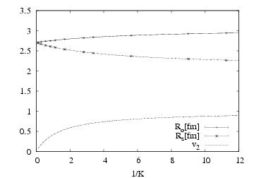
Figure 3: $R_{o}$ and $R_{s}$, averaged over the interval $0.25<p_{t}<0.75$ GeV/c, versus $1/K$, which scales like the number of collisions per particle. The lines are 3-parameter fits with Eq. (14). The dotted curve shows, for sake of illustration, the variation of elliptic flow in a non-central collision, scaled by the hydrodynamical limit (from Gombeaud:2007ub ).

Hydrodynamical calculations usually yield a value of $R_{o}/R_{s}$ which is much too large, of the order of 1.5, while RHIC data are compatible with 1. While $R_{o}$ increases with time in hydrodynamics, $R_{s}$ decreases. Initially, $R_{o}(p_{t})=R_{s}(p_{t})$ by symmetry. In the transport calculation, the same behavior is observed as the number of collisions per particle $1/K$ increases, as shown in Fig. 3. However, this increase is quite slow. The same curve shows, for sake of illustration, the increase of the elliptic flow $v_{2}$ with $1/K$ for a noncentral collision Gombeaud:2007ub . Elliptic flow converges to the “hydrodynamic limit” much faster than HBT radii. In order to put this statement on a quantitative basis, we fit our numerical results for $R_{o}(K)$ with the following formula Gombeaud:2007ub :

$$R_{o}(K)=R_{o}^{f.s.}+\frac{R_{o}^{\rm hydro}-R_{o}^{f.s.}}{1+K/K_{0}}.$$ (14)

The fit parameters are the free-streaming ($K\to\infty$) limit $R_{o}^{f.s.}$, the hydrodynamic ($K\to 0$) limit $R_{o}^{\rm hydro}$, and $K_{0}$, the value of the Knudsen number for which $R_{o}(K)$ is half-way between free-streaming and hydro. A similar formula can be used for $R_{s}(K)$. It fits our numerical results perfectly (see Fig. 3). The value of $K_{0}$ is $0.167\pm 0.007$ for $R_{o}$ and $0.215\pm 0.006$ for $R_{s}$, while it is $0.7$ for $v_{2}$ Gombeaud:2007ub : convergence toward the hydrodynamic limit requires 3-4 times more collisions for HBT radii than for elliptic flow. The other fit parameters are $R_{o}^{\rm hydro}=3.071\pm 0.006$ fm and $R_{s}^{\rm hydro}=2.088\pm 0.006$ fm: we recover the HBT puzzle $R_{o}/R_{s}\simeq 1.5$ in the hydrodynamical limit.

Figure 4: $R_{o}/R_{s}$ versus $p_{t}$ for $K=0.3$. Dashed line: thermal initial conditions, Eq. (2); full line: CGC initial conditions, Eq. (4). Error bars on the transport calculations are statistical only. Stars: data from STAR Adams:2004yc .

We now discuss the value of $R_{o}/R_{s}$ at RHIC. The centrality dependence of $v_{2}$ suggests that $K\simeq 0.3$ in central Au-Au collisions Drescher:2007cd . For this value, $v_{2}$ is already 70% of the hydrodynamic limit. On the other hand, $R_{o}/R_{s}\simeq 1.16$, which is significantly below the hydrodynamic limit of $1.5$. A similar value ($R_{o}/R_{s}\simeq 1.2$) was found with the AMPT transport code Lin:2002gc . A more detailed comparison is shown in Fig. 4, which displays $R_{o}/R_{s}$ versus $p_{t}$ for the two sets of initial conditions, Eqs. (2) and (4). $K$ has been fixed to the value which is favored by $v_{2}$ data Drescher:2007cd , i.e., $K=0.3$ for central collisions. For both sets of initial conditions, $R_{o}/R_{s}$ is essentially independent of $p_{t}$, while data show a slight decrease. In this respect, our results differ from the covariant MPC model (which is in principle equivalent to ours, with the longitudinal expansion taken into account), where $R_{o}/R_{s}$ is found smaller than 1 at large $p_{t}$ PhysRevLett.92.052301 .

Our value of $R_{o}/R_{s}$ for central collisions is in much better agreement with experimental data than models based on ideal hydrodynamics, which give a value around $1.5$. It has been recently argued that ideal hydrodynamics with an early freeze-out Broniowski:2008vp also explains the HBT puzzle. Our results also show that increasing the Knudsen number amounts to decreasing the freeze-out time in ideal hydrodynamics. Viscous corrections to ideal hydrodynamics, which incorporate deviations to local equilibrium to first order in the Knudsen number $K$, also lead to a reduced $R_{o}/R_{s}$ (together with a reduced longitudinal radius $R_{L}$, also closer to data). However, the value of $\eta/s$ required to match Romatschke:2007jx the data is much larger than that inferred from the study of elliptic flow Romatschke:2007mq , so that viscous corrections explain only a small part of the HBT puzzle Pratt:2008qv . However, viscous hydrodynamics itself breaks down at freeze-out, and may not be a reliable tool for estimating HBT radii. Our results suggest that deviations from equilibrium have larger effects on HBT radii than inferred from viscous hydrodynamics. We find that partial thermalization, which has been shown to explain the centrality dependence of $v_{2}$, also solves most of the HBT puzzle for $R_{o}/R_{s}$.

Figure 5: HBT radius $R_{o}$ versus transverse momentum $p_{t}$. Lines: our results for $K=0.3$ and different initial conditions: thermal, Eq. (2), and CGC, Eq. (4). Symbols: experimental data from STAR Adams:2004yc , PHOBOS Back:2004ug and PHENIX Adler:2004rq .

While our transport calculation gives a plausible explanation for the small $R_{o}/R_{s}$, it completely misses the absolute value of HBT radii. This is shown in Fig. 5, which displays a comparison between $R_{o}(p_{t})$ from our transport calculation with data from STAR Adams:2004yc , PHOBOS Back:2004ug and PHENIX Adler:2004rq . Experimental values are much larger. This is due to the equation of state Pratt:2008sz ; Zschiesche:2001dx , which is that of an ideal gas in our calculation. Our HBT volume $R_{o}R_{s}$ is essentially independent of the number of collisions $1/K$. It has been argued that this is a general result for an ideal gas, due to entropy conservation Akkelin:2004he . The equation of state of QCD, on the other hand, has a sharp structure around $T_{c}\sim 170$ MeV: as the temperature decreases, the entropy density drops by an order of magnitude in a narrow interval around $T_{c}$. In a heavy-ion collision, the volume increases by a large factor with essentially no change in the temperature. This explains why HBT volumes increase at the transition. A complete study must also take into account the longitudinal expansion, and its effect on the longitudinal radius $R_{L}$.

IV Azimuthally sensitive HBT

For a non-central collision, the interaction region is elliptic, and HBT radii depend on $\phi$. Azimuthally-sensitive interferometry has been investigated theoretically within hydrodynamical models Heinz:2002sq ; Tomasik:2005ny ; Frodermann:2007ab ; Csanad:2008af ; Kisiel:2008ws and transport models Humanic:2005ye . We first briefly recall why and how radii depend on $\phi$. We then study how the various radii depend on the Knudsen number. Finally, we introduce dimensionless ratios of oscillation amplitudes, which do not seem to have not been studied previously, and we compare our results with experimental data Adams:2004yc .

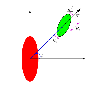
Figure 6: Illustration of $\phi$ dependent HBT radii.

Fig. 6 illustrates the $\phi$ dependence of transverse radii. The initial distribution of matter is elongated along the $y$ axis, so that $R_{o}$ has a maximum at $\phi=\pi/2$, while $R_{s}$ has a maximum at $\phi=0$. Finally, $R_{os}$ differs from zero when the principal axes of the region of homogeneity are tilted relative to the direction of momentum.

Before we present our results, let us briefly explain how the $\phi$ dependence of the radii is evaluated in the Monte-Carlo solution of the Boltzmann equation. The radii (11) involve average values, such as $\langle x_{o}\rangle$, which depend on $\phi$. Such averages can be computed by binning in $\phi$, and computing the average in each bin:

$$\langle x_{o}\rangle=\frac{\sum_{i=1}^{N}(x_{o})_{i}}{N},$$ (15)

where $N$ is the number of particles in the bin, which depends on $\phi$ due to elliptic flow. Since the $\phi$ dependence is smooth, more accurate results are obtained by fitting both the numerator and the denominator of Eq. (15) by Fourier series, using the symmetries $\phi\to-\phi$ and $\phi\to\phi+\pi$ to restrain the number of terms PhysRevC.66.044903 . Since the Fourier expansion converges rapidly, we keep terms only up to order $\cos 4\phi$ and $\sin 4\phi$.

Figure 7: Azimuthal dependence of HBT Radii. Thermal initial conditions, with $\sigma_{x}=1.95$ fm, $\sigma_{y}=2.6$ fm, corresponding roughly to a Au-Au collision at RHIC with impact parameter $b=7$ fm. The $p_{t}$ interval is the same as in Fig. 3. The Knudsen number is $K=0.4$.

Fig. 7 displays the $\phi$ dependence of $R_{o}^{2}$, $R_{s}^{2}$, and $R_{os}$. The variation of $R_{o}^{2}$ and $R_{s}^{2}$ is clearly dominated by a $\cos 2\phi$ term, while the variation of $R_{os}$ goes like $\sin 2\phi$. The mean value of $R_{o}^{2}$ is slightly higher than the mean value of $R_{s}^{2}$, which is not surprising since final-state interactions increase $R_{o}$ and decrease $R_{s}$. At $\phi=0$, however, $R_{o}<R_{s}$, reflecting the initial eccentricity of the system.

Figure 8: In-plane ($\phi=0$) and out-of-plane ($\phi=\pi/2$ radii versus $K^{-1}$ for thermal initial conditions. Initial conditions and $p_{t}$ interval as in Fig. 7. Lines are 3-parameter fits using Eq. (14).

Fig. 8 displays radii in the reaction plane ($\phi=0$) and out of the reaction plane ($\phi=\pi/2$) versus $K$. $R_{o}$ increases and $R_{s}$ decreases as the number of collisions $1/K$ increases, as already observed for central collisions (Fig. 3). Upon closer scrutiny, Fig. 8 reveals that the slope of the curves differ. This is reflected by the value of the parameter fit $K_{0}$ in Eq. (14). $K_{0}$ is largest for $R_{o}(0)$ ($K_{0}=0.38\pm 0.01$), smallest for $R_{o}(\pi/2)$ ($K_{0}=0.04\pm 0.05$), and intermediate for $R_{s}(0)$ and $R_{s}(\pi/2)$ ($K_{0}=0.26\pm 0.03$ and $0.20\pm 0.02$, respectively). Our interpretation is that thermalization is faster in plane than out of plane, which is natural since collective flow is preferentially in plane.

We now study quantitatively how oscillation amplitudes vary with $K$. There are three such amplitudes, as illustrated in Fig. 7:

$$\Delta R_{o}^{2} = R_{o}^{2}(\pi/2)-R_{o}^{2}(0)$$ (16)

$$\Delta R_{s}^{2} = R_{s}^{2}(0)-R_{s}^{2}(\pi/2)$$ (17)

$$\Delta R_{os} = R_{os}(3\pi/4)-R_{os}(\pi/4).$$ (18)

In Fig. 7, all three amplitudes are clearly comparable. If $K\gg 1$, particles escape freely after they have been produced. Setting $t=0$ in Eq. (9) and using the fact that the initial distribution is centered at $x=y=0$ and has $y\to-y$ symmetry, one easily shows that all three amplitudes are equal to $\langle y^{2}-x^{2}\rangle$. The results are integrated over the $p_{t}$ range $0.25<p_{t}<0.75$ GeV/c, but our results depend weakly on $p_{t}$. In particular, we do not see the inversion of oscillations at large $p_{t}$ reported in earlier hydrodynamical calculations Heinz:2002sq ; Frodermann:2007ab . This inversion was not observed in more recent calculations Kisiel:2008ws .

Figure 9: Ratios of oscillation amplitudes versus $K^{-1}$ for thermal initial conditions. $R_{o}^{2}$, $R_{s}^{2}$ and $R_{os}$ are integrated over the $p_{t}$ interval $0.5<p_{t}<0.75$ GeV/c. Lines are drawn to guide the eye.

Oscillation amplitudes scale like the eccentricity of the overlap area between the two nuclei, which depends on centrality and is not known directly. This dependence can be avoided by considering ratios of oscillation amplitudes. Out of $3$ amplitudes, one may construct $2$ ratios, $\Delta R_{os}/\Delta R_{o}^{2}$ and $\Delta R_{o}^{2}/\Delta R_{s}^{2}$. These ratios can be extracted directly from experimental data, and are equal to unity in the free-streaming limit (large $K$). They are plotted in Fig. 9 versus $1/K$. Final-state interactions increase the oscillations of $R_{o}$ relative to $R_{s}$, much in the same way as they increase $R_{o}$ relative to $R_{s}$ for central collisions. The opposite behavior was found in hydro Frodermann:2007ab and blast-wave Retiere:2003kf calculations, and we do not understand the origin of this discrepancy.

For realistic values of $K$, both ratios deviate little from unity. It is also interesting to compare the eccentricity seen in HBT radii, for instance in $R_{s}$:

$$\epsilon_{s}\equiv\frac{R_{s}^{2}(0)-R_{s}^{2}(\pi/2)}{R_{s}^{2}(0)+R_{s}^{2}(\pi/2)}$$ (19)

with the initial eccentricity

$$\epsilon=\frac{\sigma_{y}^{2}-\sigma_{x}^{2}}{\sigma_{y}^{2}+\sigma_{x}^{2}}.$$ (20)

In the limit $K\to\infty$, $\epsilon_{s}$ and $\epsilon$ are strictly equal for both sets of initial conditions. The ratio $\epsilon_{s}/\epsilon$ is plotted in Fig. 9. It also remains close to unity. We conclude that none of the observables we can construct from oscillation amplitudes is an interesting probe of thermalization. For realistic values of $K$, the region of homogeneity essentially retains the shape of the initial distribution.

	STAR data	our results
		$K=0.32$	$K=0.51$
$\Delta R_{o}^{2}/\Delta R_{s}^{2}$	$1.45\pm 0.61$	$1.08\pm 0.02$	$1.05\pm 0.02$
$\Delta R_{os}/\Delta R_{o}^{2}$	$0.68\pm 0.42$	$0.97\pm 0.03$	$0.99\pm 0.03$
$\epsilon_{s}$	$0.080\pm 0.026$	$0.205\pm 0.003$	$0.213\pm 0.005$

	STAR data	our results
		$K=0.31$	$K=0.49$
$\Delta R_{o}^{2}/\Delta R_{s}^{2}$	$1.09\pm 0.46$	$1.14\pm 0.02$	$1.06\pm 0.02$
$\Delta R_{os}/\Delta R_{o}^{2}$	$0.65\pm 0.31$	$0.90\pm 0.04$	$0.92\pm 0.04$
$\epsilon_{s}$	$0.086\pm 0.017$	$0.172\pm 0.005$	$0.174\pm 0.005$

Table 1: Comparison between results from STAR Adams:2004yc and our calculations. Top: centrality interval 20-30% and $k_{t}\in[0.15,0.25]$ GeV/c. Bottom: centrality interval 10-20% and $k_{t}\in[0.35,0.45]$ GeV/c.

Although our model calculation is too crude to reproduce the magnitude of HBT radii, we expect that the above ratios are less model dependent; in particular, they all go to 1 in the absence of final-state interactions. A comparison with existing data is therefore instructive. Table 1 displays comparisons between our results and experimental data from STAR Adams:2004yc . The correspondence between centrality and eccentricity was taken from Kolb:2001qz . For each set of data, the two values of the Knudsen number span the range inferred from the centrality dependence of $v_{2}$ Drescher:2007cd . Note that the $p_{t}$ ranges differ for the two centrality intervals. This is the reason why our results are also slightly different, although the values of $K$ are essentially the same. Our results for $\Delta R_{o}^{2}/\Delta R_{s}^{2}$ and $\Delta R_{os}/\Delta R_{o}^{2}$ are compatible with experimental data, but the latter have large error bars. On the other hand, the experimental value of $\epsilon_{s}$ is smaller by a factor 2 than our value. In our calculations, $\epsilon_{s}$ remains very close to the initial eccentricity (see Fig. 9). Experimentally, however, the initial eccentricity seems to be washed out by the expansion. This is a spectacular effect, whose importance doesn’t seem to have been fully appreciated so far. Hydrodynamical calculations have been reported Kisiel:2008ws which are in fair agreement with the measured value of $\epsilon_{s}$. These calculations use a soft equation of state: it is likely that the soft equation of state of QCD is responsible for the reduced eccentricity seen in data.

V Conclusions

We have carried out a systematic study of how HBT observables evolve with the degree of thermalization in the system, characterized by the Knudsen number $K$. The number of collisions per particle scales like $1/K$, and local equilibrium corresponds to the limit $K\to 0$. Our results show that HBT observables depend very weakly on $K$:

• A decrease of $R_{o}$ with $p_{t}$ is expected from initial conditions; collective flow only makes this decrease slightly stronger.

• The ratio $R_{o}/R_{s}$ increases very slowly when one approaches the hydrodynamical limit. For the values of $K$ found in Ref. Drescher:2007cd , it is lower than $1.2$, and much lower than predicted by hydrodynamics. Partial thermalization solves most of the HBT puzzle.

• For non-central collisions, the variations of $R_{o}^{2}$, $R_{s}^{2}$ and $R_{os}$ with azimuth have almost equal amplitudes. The final eccentricity seen in the side radius $R_{s}^{2}$ is very close to the initial eccentricity.

Our results are in quantitative agreement with data for $R_{o}/R_{s}$, $\Delta R_{os}/\Delta R_{o}^{2}$ and $\Delta R_{o}^{2}/\Delta R_{s}^{2}$. On the other hand, our absolute values for $R_{o}$ and $R_{s}$ are much too small. Experimentally, it is also found that the final eccentricity is smaller than the initial eccentricity, almost by a factor 2. Both effects cannot be due to flow alone. On the other hand, they might be a signature of the softness of the QCD equation of state or, equivalently, of the transition from a quark-gluon plasma to a hadron gas. When the quark-gluon plasma transforms into hadrons, the volume of the system increases by a large factor: the source swells, which results in larger radii and a smaller eccentricity.

References

- (1) M. A. Lisa, S. Pratt, R. Soltz and U. Wiedemann, Ann. Rev. Nucl. Part. Sci. 55, 357 (2005), [arXiv:nucl-ex/0505014].
- (2) S. V. Akkelin and Y. M. Sinyukov, Phys. Lett. B356, 525 (1995).
- (3) R. H. Brown and R. Q. Twiss, Nature 177, 27 (1956).
- (4) F. Retiere and M. A. Lisa, Phys. Rev. C70, 044907 (2004), [arXiv:nucl-th/0312024].
- (5) P. F. Kolb and U. W. Heinz, arXiv:nucl-th/0305084.
- (6) T. Hirano and K. Tsuda, Phys. Rev. C66, 054905 (2002), [arXiv:nucl-th/0205043].
- (7) D. Zschiesche, S. Schramm, H. Stoecker and W. Greiner, Phys. Rev. C65, 064902 (2002), [arXiv:nucl-th/0107037].
- (8) J. Socolowski, O., F. Grassi, Y. Hama and T. Kodama, Phys. Rev. Lett. 93, 182301 (2004), [arXiv:hep-ph/0405181].
- (9) P. Huovinen and P. V. Ruuskanen, Ann. Rev. Nucl. Part. Sci. 56, 163 (2006), [arXiv:nucl-th/0605008].
- (10) P. Romatschke, Eur. Phys. J. C52, 203 (2007), [arXiv:nucl-th/0701032].
- (11) S. Pratt, arXiv:0811.3363 [nucl-th].
- (12) Z.-w. Lin, C. M. Ko and S. Pal, Phys. Rev. Lett. 89, 152301 (2002), [arXiv:nucl-th/0204054].
- (13) D. Molnár and M. Gyulassy, Phys. Rev. Lett. 92, 052301 (2004).
- (14) Q. Li, M. Bleicher and H. Stoecker, Phys. Rev. C73, 064908 (2006).
- (15) C. Gombeaud and J.-Y. Ollitrault, Phys. Rev. C77, 054904 (2008), [arXiv:nucl-th/0702075].
- (16) F. Karsch and E. Laermann, arXiv:hep-lat/0305025.
- (17) A. Krasnitz, Y. Nara and R. Venugopalan, Phys. Rev. Lett. 87, 192302 (2001), [arXiv:hep-ph/0108092].
- (18) T. Lappi, Phys. Rev. C67, 054903 (2003), [arXiv:hep-ph/0303076].
- (19) L. D. McLerran and R. Venugopalan, Phys. Rev. D49, 2233 (1994), [arXiv:hep-ph/9309289].
- (20) A. Krasnitz, Y. Nara and R. Venugopalan, Nucl. Phys. A727, 427 (2003), [arXiv:hep-ph/0305112].
- (21) T. Lappi, Eur. Phys. J. C55, 285 (2008), [arXiv:0711.3039 [hep-ph]].
- (22) PHENIX, S. S. Adler et al., Phys. Rev. C69, 034909 (2004), [arXiv:nucl-ex/0307022].
- (23) R. S. Bhalerao, J.-P. Blaizot, N. Borghini and J.-Y. Ollitrault, Phys. Lett. B627, 49 (2005), [arXiv:nucl-th/0508009].
- (24) H.-J. Drescher, A. Dumitru, C. Gombeaud and J.-Y. Ollitrault, Phys. Rev. C76, 024905 (2007), [arXiv:0704.3553 [nucl-th]].
- (25) Z.-W. Lin, C. M. Ko, B.-A. Li, B. Zhang and S. Pal, Phys. Rev. C72, 064901 (2005), [arXiv:nucl-th/0411110].
- (26) P. Huovinen and D. Molnar, Phys. Rev. C79, 014906 (2009), [arXiv:0808.0953 [nucl-th]].
- (27) M. L. Miller, K. Reygers, S. J. Sanders and P. Steinberg, Ann. Rev. Nucl. Part. Sci. 57, 205 (2007), [arXiv:nucl-ex/0701025].
- (28) A. N. Makhlin and Y. M. Sinyukov, Z. Phys. C39, 69 (1988).
- (29) J. Y. Ollitrault, NATO Sci. Ser. II 87, 237 (2002).
- (30) J.-Y. Ollitrault, Phys. Rev. D46, 229 (1992).
- (31) STAR, J. Adams et al., Phys. Rev. C71, 044906 (2005), [arXiv:nucl-ex/0411036].
- (32) W. Broniowski, M. Chojnacki, W. Florkowski and A. Kisiel, Phys. Rev. Lett. 101, 022301 (2008), [arXiv:0801.4361 [nucl-th]].
- (33) P. Romatschke and U. Romatschke, Phys. Rev. Lett. 99, 172301 (2007), [arXiv:0706.1522 [nucl-th]].
- (34) PHOBOS, B. B. Back et al., Phys. Rev. C73, 031901 (2006), [arXiv:nucl-ex/0409001].
- (35) PHENIX, S. S. Adler et al., Phys. Rev. Lett. 93, 152302 (2004), [arXiv:nucl-ex/0401003].
- (36) S. Pratt and J. Vredevoogd, Phys. Rev. C78, 054906 (2008), [arXiv:0809.0516 [nucl-th]].
- (37) S. V. Akkelin and Y. M. Sinyukov, Phys. Rev. C70, 064901 (2004).
- (38) U. W. Heinz and P. F. Kolb, Phys. Lett. B542, 216 (2002), [arXiv:hep-ph/0206278].
- (39) B. Tomasik, AIP Conf. Proc. 828, 464 (2006), [arXiv:nucl-th/0509100].
- (40) E. Frodermann, R. Chatterjee and U. Heinz, J. Phys. G34, 2249 (2007), [arXiv:0707.1898 [nucl-th]].
- (41) M. Csanad, B. Tomasik and T. Csorgo, Eur. Phys. J. A37, 111 (2008), [arXiv:0801.4434 [nucl-th]].
- (42) A. Kisiel, W. Broniowski, M. Chojnacki and W. Florkowski, Phys. Rev. C79, 014902 (2009), [arXiv:0808.3363 [nucl-th]].
- (43) T. J. Humanic, Int. J. Mod. Phys. E15, 197 (2006), [arXiv:nucl-th/0510049].
- (44) U. Heinz, A. Hummel, M. A. Lisa and U. A. Wiedemann, Phys. Rev. C 66, 044903 (2002).
- (45) P. F. Kolb, U. W. Heinz, P. Huovinen, K. J. Eskola and K. Tuominen, Nucl. Phys. A696, 197 (2001), [arXiv:hep-ph/0103234].