Effective Delay Control in Online Network Coding

Abstract

Motivated by streaming applications with stringent delay constraints, we consider the design of online network coding algorithms with timely delivery guarantees. Assuming that the sender is providing the same data to multiple receivers over independent packet erasure channels, we focus on the case of perfect feedback and heterogeneous erasure probabilities. Based on a general analytical framework for evaluating the decoding delay, we show that existing ARQ schemes fail to ensure that receivers with weak channels are able to recover from packet losses within reasonable time. To overcome this problem, we re-define the encoding rules in order to break the chains of linear combinations that cannot be decoded after one of the packets is lost. Our results show that sending uncoded packets at key times ensures that all the receivers are able to meet specific delay requirements with very high probability.

I Introduction

The issue of delay between data transmission and successful delivery to the receiving application is arguably one of the key concerns when applying coding ideas to networking problems. This is particularly true for network coding, where nodes combine multiple packets by means of algebraic operations and perform computationally heavy Gaussian elimination algorithms to recover the sent data. Although there is growing consensus that both in wireless broadcast scenarios [1, 2] network coding can bring benefits in terms of throughput and robustness, the fact that a receiver may have to wait for a considerable number of packets, before it can decode the data, justifies the question whether and how network coding can be used in scenarios with stringent end-to-end delays.

In the seminal paper of Ahlswede, Cai, Li, and Yeung [3], which shows that network coding is required to achieve the multicast capacity of a general network, the problem is formulated in an information-theoretic setting, where delay and complexity are not taken into account. Delay is also not a primary concern of the algebraic framework in [4] and of the random linear network coding method [5, 6], in which each node in the network selects independently and randomly a set of coefficients and uses them to form linear combinations of the data symbols (or packets) it receives. When intermediate nodes cannot perform coding operations and applications are able to tolerate some delay, fountain codes (e.g., Raptor codes [7]) emerge as a viable solution offering low coding overhead as well as near-optimal throughput over packet erasure channels.

Clearly, in all of these instances, coding is performed in a feedforward fashion. The encoders upstream are oblivious to packet loss downstream and their coding decisions do not exploit any feedback information. In contrast, the property that transmitted packets are linear combinations of subsets of packets available at the sender buffer suggests that network coding protocols could be enhanced by modifying the content of the acknowledgments typically provided by transport protocols. Instead of acknowledging specific packets, each destination node of a unicast or multicast session can send back requests for degrees of freedom that increase the dimension of its vector space and allow for faster decoding.

Recent contributions that pursue this idea (e.g., [8, 9]) focus mostly on end-to-end reliability with perfect feedback, i.e., complete and immediate knowledge of the packets stored at each receiver. The source node reacts by sending the most innovative linear combination that is useful to most destination nodes. Throughput optimal network coding protocols following this concept appear in [10, 11], which introduce the useful notion of seen packet as an abstraction for the case in which a packet cannot yet be decoded but can be safely removed from the sender buffer. Removing packets in a timely fashion has obvious benefits in terms of queue length. By using the feedback information to move a coding window along the sender buffer instead of mixing fixed sets of packets (also called generations [6]), these protocols perform online network coding in the sense that they adapt their coding decisions based on the erasure patterns observed in the network.

Realizing that existing solutions do not yet cover the full range of trade-offs between throughput and delay, in particular when users experience different packet loss probabilities, we set out to provide end-to-end delay control for online network coding with feedback. Our main contributions are as follows:
$\bullet$ Delay Analysis: We provide an analytical framework to evaluate the delay performance of online network coding algorithms that leverage feedback for increased reliability. The novelty of our approach lies in observing how each erasure event affects the chains of undecoded linear combinations that build up at the receiver buffer. Moreover, we can map the information backlog between receivers to an appropriate random walk on a high dimensional lattice, which brings further insight into the delay behavior.
$\bullet$ Online Network Coding Algorithms with Delay Constraints: Using the knowledge of the chain length at each receiver, we identify simple ways of limiting the delay by means of informed encoding decisions. In particular, we show the benefits of sending uncoded packets to alleviate the delay of weaker receivers.

Our work differs from [10] in that we consider heterogeneous users with different erasure probabilities and take the end-to-end delay to be our main figure of merit. Also centered around equal erasure probabilities for all users, the contribution in [11] focuses on the two user case and uses only the binary field, whereas, in contrast also with [9], we consider also larger field sizes and larger number of users. A different method to limit the delay is to mix packets in such a way that at least some of the receivers are able to decode a symbol immediately upon receiving a new packet. If no feedback information is available, the best one can do is to choose the packets randomly and optimize only the number of packets to be combined [12], an approach which appears adequate for highly constrained scenarios such as data preservation in sensor networks. Results on the optimum degree distributions with respect to network dynamics and topology can be found in [13]. The use of feedback under similar assumptions was explored in [14]. The main difference between [14] and this contribution is that here we provide analytical results, consider higher fields and do not enforce immediate decoding. We believe that our algorithms are able to reach a larger set of operating points in the delay-throughput plane and are thus well suited for streaming applications with stringent delay requirements, where network coding has already proved to yield competitive solutions (see, e.g., [15]).

The remainder of the paper is organized as follows. Section II introduces terminology and describes the core ideas of online network coding with feedback. Our analytical framework for evaluating the end-to-end delay is outlined in Section III with results on the relationship between erasure patterns, undecodable chains, and incurred delays. Section IV provides solutions for effective delay control and the corresponding performance results are presented in Section V. In Section VI, we briefly discuss the implications of imperfect feedback and conclude the paper in Section VII.

II Essential Background

II-A System Setup

Suppose that a single queue sender wants to transmit a stream of packets to multiple receivers. For simplicity, we assume that packets arrive at the sender in a certain order (older packets first) and are readily available at the sender for encoding and transmission. Each receiver $i$ is connected to the sender via a separate packet erasure channel, which takes one packet per time slot and loses a packet with probability $\epsilon_{i}$. Packets are lost independently across channels and time slots and receivers are able to detect when a packet is missing. Since the sender has access to perfect feedback (without errors, losses, or delay), it can make encoding decisions based on the buffer state of each receiver.

II-B ARQ for Network Coding

The reference system for our analysis is the ARQ for network-coding (ANC) scheme presented in [10], which was shown to be throughput optimal for the case of Poisson arrivals, perfect feedback, and identical erasure probabilities on all channels. In this scheme, the sender transmits linear combinations of the packets in its queue, where the decision which packets to combine relies on the concept of seen packets. A packet ${\bf p}$ is said to be seen by a receiver, if the receiver is able to construct a linear combination of the form ${\bf p}+{\bf q}$, such that ${\bf q}$ is a linear combination of packets that are newer than ${\bf p}$. In particular, a packet is seen when it can be decoded. The sender always transmits a packet that is a combination of the last (i.e., oldest) unseen packets of each of the receivers. This ensures that the last unseen packet will now be seen by all receivers which receive the coded packet.

A packet can be dropped from the sender queue whenever it was seen (but not necessarily decoded) by all receivers. This has the agreeable property that queue sizes at the sender are kept small, since the sender can drop packets before they are decoded at all receivers, without compromising reliability. The expected queue size was shown to be $O((1-\epsilon)^{-1})$ [10]. The basic operation of this scheme is illustrated in Table I, which lists the sequence of packet receptions (OK) and erasures (E) and shows the corresponding coding decisions made by the sender for a two receiver case. This example shall be discussed in more detail below and in the next section.

The scheme in [10] was extended in [11] with the goal of reducing the decoding delay, specifically for the two receiver scenario. Here, packets that are unseen at a receiver because all combinations containing that packet were lost are requested by the receiver at a later stage. In the example of Table I, this happens in time slot 7, where receiver 2 requests ${\bf p_{6}}$, instead of ${\bf p_{5}}$, resulting in the transmission of ${\bf p_{6}}\oplus{\bf p_{7}}$. Packet ${\bf p_{5}}$ is only requested in time slot 9, after receiver 2 decoded ${\bf p_{6}}$.

TABLE I: Example of Online Network Coding with ARQ

Time Slot	Sent Packet	Receiver 1	Receiver 2
1	${\bf p_{1}}$	OK	E
2	${\bf p_{1}}\oplus{\bf p_{2}}$	OK	OK
3	${\bf p_{2}}\oplus{\bf p_{3}}$	OK	OK
4	${\bf p_{3}}\oplus{\bf p_{4}}$	OK	OK
5	${\bf p_{4}}\oplus{\bf p_{5}}$	OK	E
6	${\bf p_{4}}\oplus{\bf p_{6}}$	OK	OK
7	${\bf p_{6}}\oplus{\bf p_{7}}$	E	OK
8	${\bf p_{7}}$	OK	OK
9	${\bf p_{5}}\oplus{\bf p_{8}}$	OK	OK
10	${\bf p_{8}}\oplus{\bf p_{9}}$	E	OK
11	${\bf p_{9}}$	OK	E
12	${\bf p_{9}}\oplus{\bf p_{10}}$	OK	OK

III Delay Analysis

Before proceeding with the analysis, it is important to clarify the notion of delay in the context of online network coding algorithms. Once an information packet ${\bf p}$ arrives at the sender queue it will typically go through five different stages: (1) ${\bf p}$ is mixed with other packets by means of coding operations, (2) ${\bf p}$ is transmitted to the receivers, (3) ${\bf p}$ is seen by the receiver, (4) ${\bf p}$ is decoded, and (5) ${\bf p}$ is delivered to the application. In the following we shall focus on the decoding delay, which is measured as the number of slots between the first transmission of an encoding of the packet and successful decoding at the receiver. Clearly, this delay subsumes the time it takes for a packet to be seen and the time it takes for a seen packet to be decoded.

III-A Two Receivers

We start with the case of two receivers and assume without loss of generality that the sender restricts its transmissions to uncoded packets or XORs of two packets [10]. Since we assume that all packets that are necessary for encoding are readily available at the sender, the incurred decoding delay depends only on the rules enforced by the online network coding algorithm and the erasure patterns of the two channels. In each time slot we have one of the erasure events listed in Table II, which occur with the given event probabilities.

TABLE II: List of Possible Erasure Events

Event	Description	Probability
$A$	No erasures	$P(A)=(1-\epsilon_{1})(1-\epsilon_{2})$
$B$	Receiver 1 gets the coded packet and receiver 2 observes an erasure	$P(B)=(1-\epsilon_{1})\epsilon_{2}$
$C$	Receiver 1 observes an erasure and receiver 2 gets the coded packet	$P(C)=\epsilon_{1}(1-\epsilon_{2})$
$D$	Both receivers observe an erasure	$P(D)=\epsilon_{1}\epsilon_{2}$

An erasure event causes a receiver buffer to build up a chain of length $K$, which we define as a set of $K$ independent linear combinations involving $L>K$ symbols, which cannot be decoded by the receiver. In the scenario shown in Table I, receiver 2 suffers from losses (denoted by E) in time slots 1 and 5, whereas receiver 1 obtains everything error free (OK) except for the data transmitted in slot 7. Each erasure sets a mark for a new chain of undecodable linear combinations, such that each chain begins immediately after its preceding chain has been solved. For example, up to slot 4 receiver 2 built up the chain $\{{\bf p_{1}}\oplus{\bf p_{2}},{\bf p_{2}}\oplus{\bf p_{3}},{\bf p_{3}}\oplus{\bf p_{4}}\}$. The erasure in slot 5 sets a mark for a new chain, which will involve ${\bf p_{5}}$ by necessity. However, before that chain begins, the first chain grows to $\{{\bf p_{1}}\oplus{\bf p_{2}},{\bf p_{2}}\oplus{\bf p_{3}},{\bf p_{3}}\oplus{\bf p_{4}},{\bf p_{4}}\oplus{\bf p_{6}},{\bf p_{6}}\oplus{\bf p_{7}}\}$. Since receiver 1 experiences an erasure in slot 7, the encoding rule forces the sender to transmit packet ${\bf p_{7}}$ in uncoded fashion, which in turn allows receiver 2 to break its first chain and recover packets $\{{\bf p_{1}},{\bf p_{2}},{\bf p_{3}},{\bf p_{4}},{\bf p_{6}},{\bf p_{7}}\}$. The second chain begins immediately in slot 9 with $\{{\bf p_{5}}\oplus{\bf p_{8}}\}$, because packet $\bf p_{5}$ was not seen by receiver 2 in slot 5. Note that an erasure event at the leading receiver 1 is not enough to allow receiver 2 to break the current chain. If the following packet is lost at receiver 2, as shown in the example with the loss of ${\bf p_{2}}$ in time slot 11, the chain will simply continue to grow.

Clearly, the decoding delay is deeply influenced by the length of chains such as these and by the sender’s ability to break them in a timely manner — in spite of randomly occurring packet erasures

III-A1 First-Order Analysis

Assuming that channels 1 and 2 have erasure probabilities $\epsilon_{1}$ and $\epsilon_{2}$, respectively, and that the sender follows the simple ARQ rules outlined in Section II, we can describe the chain duration in a probabilistic fashion.

Proposition 1

After an erasure of type $B$ that starts a chain at receiver 2, the chain remains unbroken for a duration of $T$ slots with probability

$$P(T) = \epsilon_{1}(1-\epsilon_{2})^{2}\sum_{t_{1}=0}^{T-1}(\epsilon_{1}\epsilon_{2})^{t_{1}}\cdot$$ (1)

$$\cdot\sum_{t_{2},t_{3}:2t_{2}+t_{3}=T-1-t_{1}}(\epsilon_{1}\epsilon_{2}(1-\epsilon_{1})(1-\epsilon_{2}))^{t_{2}}\cdot(1-\epsilon_{1})^{t_{3}}.$$

Proof:

We start by observing that events of type $D$ only increase the delay until the chain can be decoded but do not otherwise affect the recovery process or the length of the chain. Therefore, there is nothing to lose from ignoring events of type $D$ for now and taking their impact into account only at a later stage. If we only take into account events of type $A$, $B$ or $C$, a chain starting with an erasure is only broken after an erasure event of type $C$ (in which receiver 2 obtains a packet missed by receiver 1) immediately followed by an event of type $A$ or $C$, in which receiver 2 obtains the uncoded symbol that will ultimately allow it to decode the chain. While the chain is unbroken, any occurrence of event pairs that are not $CC$ or $CA$ will add to the duration of the chain. Any occurrence of $D$ at any slot (including between the first and second events of the pairs we considered previously) will further increase the chain duration.

Since the channel erasures are independent from slot to slot, we can think of all the occurrences of $D$, none of which affects the breaking of the chain in any way, as a contiguous block in the first slots after the erasure. With this assumption in mind, notice that for the chain to be broken $T+1$ slots after the erasure, in slot $T$ we must observe $C$, since the only pairs that break a chain are $CA$ and $CC$. Thus, after the first slots (where $D$ was observed) and up to and including slot $T-2$, if we observe a $C$, it must be followed by the event $B$. Regarding the remaining slots, we can have isolated events $A$ and $B$ (only the ones not preceded by $C$, because those are already taken into account). Therefore, letting $t_{1}$, $t_{2}$ and $t_{3}$ represent the number of occurrences of the events $D$, $CB$ and $A\cup B$, respectively, we have that

$$P(T) = \sum_{t_{1}=0}^{T-1}P(D)^{t_{1}}\sum_{t_{2},t_{3}:2t_{2}+t_{3}=T-1-t_{1}}P(CB)^{t_{2}}(P(A)+P(B))^{t_{3}}\cdot$$ (2)

$$\cdot(P(CA)+P(CC))$$

Notice that, since erasures in different slots are independent of each other, we have that $P(CA)=P(C)P(A)$, $P(CB)=P(C)P(B)$ and $P(CC)=P(C)^{2}$. Thus, substituting $P(A)$, $P(B)$ and $P(D)$ by the expressions in Table II in (2) and simplifying the resulting terms we obtain Equation (1). ∎

Likewise, we can compute the distribution for the chains built up at the other receiver.

Proposition 2

After an erasure of type $C$, a chain at receiver 1 remains unbroken for a duration of $T$ slots with probability

$$P(T) = \epsilon_{2}(1-\epsilon_{1})^{2}\sum_{t_{1}=0}^{T-1}(\epsilon_{1}\epsilon_{2})^{t_{1}}\cdot$$ (3)

$$\cdot\sum_{t_{2},t_{3}:2t_{2}+t_{3}=T-1-t_{1}}(\epsilon_{1}\epsilon_{2}(1-\epsilon_{1})(1-\epsilon_{2}))^{t_{2}}\cdot(1-\epsilon_{2})^{t_{3}}.$$

Proof:

The proof follows analogously to the previous proof by swapping events $B$ and $C$. ∎

III-A2 Higher-Order Analysis

As mentioned earlier, if a second erasure of type $B$ occurs while receiver 2 is still processing an unbroken chain, the result can be viewed as a marker that signals a future new chain. This second chain will begin immediately after the receiver recovered from the current chain. From then on, the distribution of the number of slots required to break it is also given by Proposition 1. The delay with which receiver 2 sees (and later decodes) the packet missed in the second erasure will naturally be dependent on the number of slots that pass between the second erasure and the breaking of the first chain. A similar argument applies to the $k$th erasure event that takes place while receiver 1 is recovering from the first chain. The result is a marker for a $k$th chain, whose overall delay is given by $D=\sum_{i=0}^{k}T_{i}$, where $T_{0}$ is the number of slots between the $k$th erasure and the breaking of the first chain and $T_{i}$ denotes the time it takes to break chain $i$. Notice that $T_{0}$ follows the same distribution as $T_{i}$, because it counts the time slots between an erasure and the breaking of a chain. Clearly, $D$ results from the sum of the independent and identically distributed random variables $T_{0},T_{1},\dots,T_{k}$, and for this reason is itself a random variable.

III-B Multiple Receivers

As should be expected, determining the various forms of delay becomes increasingly complex for larger numbers of receivers. To gain some insight, we start by observing that, at any point in time there will be at least one leader, where leader(s) at time slot $t$ are one or more of the receivers which have received the maximum number of packets up to time slot $t$. The following proposition describes an important property of the leader status.

Proposition 3

A receiver that became a leader at time $t$ and stays in the group of leaders until it receives one more packet at time $t+\delta$ is able to decode all packets included in any of the linear combinations transmitted until $t+\delta$. A receiver continues to be able to decode immediately all coded packets at $t^{\prime}>t+\delta$, provided it remains the leader or a member of the group of leaders.

Proof:

Assume the leaders lose a packet at time $t$ (otherwise no other receiver can become a leader) and suppose that they received the first $d$ packets up to that time. These packets carry encodings of at most the first $d+1$ information units. This ensures that leaders would have been able to decode a new packet, had they received the current transmission. A new receiver is now to become part of the leaders receives its next packet at time $t+\delta$ (and thus no other leaders receive a packet between $t$ and $t+\delta$). Since the coding algorithms are throughput optimal (i.e., each received packet is innovative) the receiver will have $d+1$ (coded) packets which are combinations of the first $d+1$ original packets. It can thus solve the corresponding system of linear equations and decode all packets. ∎

As shown in the example of Table I for time slot 8, also non-leaders may break chains and decode packets. However, as the number of receivers increases and/or the erasure probabilities become more heterogeneous, the probability that non-leaders can decode becomes very small.

We use the fact that leaders can decode all packets to derive an upper bound on the decoding delay in the multiple receiver case. As we have seen, the decoding delay is tightly connected to the time interval between the moment in which a receiver ceases to be a leader and the moment it is able to catch up and regain the leader status. Describing the system in terms of the packets received by each of the receivers leads to a state space which grows exponentially in the number of receivers and is therefore intractable.

However, taking the point of view of one of the receivers, for instance $R_{1}$, we can describe the evolution of the differences in received packets between $R_{1}$ and the remaining receivers as a random walk in an $(n-1)$-dimensional lattice, where $n$ is the number of receivers. To develop some intuition, consider the case of three receivers, denoted $R_{1}$, $R_{2}$, and $R_{3}$. Let $x_{1}$ denote the difference of received packets between $R_{1}$ and $R_{2}$, and let $x_{2}$ describe the difference between $R_{1}$ and $R_{3}$. The state of the system from the perspective of $R_{1}$ is thus described by the pair $(x_{1},x_{2})$, which can be viewed as a point in two-dimensional space. In each time slot, there are eight possible erasure events, depending on whether each of the receivers suffers a packet loss or not. If, in a given time slot, all receivers lose a packet or if there are no packet losses, then the state does not change. In all other cases, $x_{1}$ and $x_{2}$ will increase or decrease by one unit according to the transition rules in Table III, where once again we use OK and E to denote successful reception and packet erasure, respectively.

TABLE III: Transition Rules for the Three-Receiver Case

Event	$R_{1}$	$R_{2}$	$R_{3}$	Next State	Direction
$E_{0}$	OK	OK	OK	$(x_{1},x_{2})$	$\cdot$
$E_{1}$	OK	OK	E	$(x_{1},x_{2}+1)$	$\uparrow$
$E_{2}$	OK	E	OK	$(x_{1}+1,x_{2})$	$\rightarrow$
$E_{3}$	OK	E	E	$(x_{1}+1,x_{2}+1)$	$\nearrow$
$E_{4}$	E	OK	OK	$(x_{1}-1,x_{2}-1)$	$\swarrow$
$E_{5}$	E	OK	E	$(x_{1}-1,x_{2})$	$\leftarrow$
$E_{6}$	E	E	OK	$(x_{1},x_{2}-1)$	$\downarrow$
$E_{7}$	E	E	E	$(x_{1},x_{2})$	$\cdot$

Once we associate the erasure events with the corresponding probabilities, which can be easily computed from the erasure probabilities for each of the receivers, we obtain a random walk on a two-dimensional lattice, as illustrated in Figure 1.

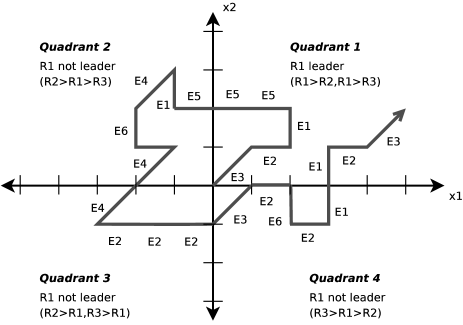
Figure 1: Random walk interpretation of the state evolution at receiver $R_{1}$.

Clearly, $R_{1}$ is a leader if and only if the coordinates $(x_{1},x_{2})$ lie in the first quadrant. In this case, $x_{1}$ and $x_{2}$ are both positive (or zero) and $R_{1}$ has received either the same or a higher number of packets than the other receivers. $R_{1}$ ceases to be a leader, when its state position moves from the first quadrant to one of the other three. Conversely, it becomes a leader again if its state position moves back to quadrant one. The length of time $R_{1}$ spends in each of the quadrants depends only on the erasure probabilities, or equivalently the probabilities of erasure events $E_{1}\dots E_{7}$.

The proposed random walk model proves to be very useful for computing upper bounds on the decoding delay experienced by receiver $R_{1}$. When $(x_{1},x_{2})$ is in the first quadrant, we have that $R_{1}$ is the leader and, thus, by Proposition 3, every received packet is immediately decoded, which is equivalent to zero delay. Therefore, if $n$ is the number of slots in which $R_{1}$ is a leader and $e$ is the number of erasures observed by $R_{1}$ during those slots, $n-e$ packets have zero delay.

When $(x_{1},x_{2})$ lies outside the first quadrant (or, equivalently, when $R_{1}$ is not a leader), we can upper bound the delay of the packets transmitted in those slots as follows. Let $t_{1}$ be a time slot such that $(x_{1},x_{2})$ is in the first quadrant at slot in slot $t_{1}-1$ and elsewhere in slot $t_{1}$. Furthermore, let $t_{2}$ be the first time slot after $t_{1}$ such that $(x_{1},x_{2})$ is again in the first quadrant in slot $t_{2}+1$. This means that during the slots between $t_{1}$ and $t_{2}$, $R_{1}$ is not a leader. In the worst case, by Proposition 3, all the packets transmitted between $t_{1}$ and $t_{2}$ will only be decoded at slot $t_{2}+1$. Hence, we can upper bound the delay of all these packets by $t_{2}-t_{1}$.

It is worth pointing out that generalizing this idea from three receivers to $n$ receivers forces us to consider random walks in $n$-dimensional lattices. The class of random walks we need can be deemed as untypical on several counts: (a) they assign non-uniform probabilities to different directions by virtue of the properties of online network coding, and (b) they admit the possibility that a node stays in the same position. Close inspection of the related literature in probability theory reveals that the complete mathematical characterization of integer random walks — even for uniform distributions in two dimensions — offers non-trivial difficulties. A large body of work is concerned with the number of points covered by the random walk up to a certain time (see e.g. [16]), other contributions focus on hitting times on the coordinate axis [17] or among multiple random walks  [18]. At this time, providing a mathematical description of the crossing times between quadrants of a non-uniform random walk is clearly a daunting task, which justifies the use of numerical techniques at the final stage of the proposed analysis.

Returning to the three-node case, Fig. 2 illustrates the upper bounds on the decoding delay of receiver $R_{1}$ we obtain using the proposed methodology. As was to be expected, the behavior of the cumulative distribution function can be very different depending on whether the erasure probability of the receiver of interest is equal to the erasure probabilities of the other receivers, or lower, or higher. With a higher erasure probability, as shown in the bottom curve with $\epsilon_{1}=0.25$, $\epsilon_{2}=0.2$, and $\epsilon_{3}=0.1$, almost all of the chains are broken only after the leading receivers have received all of their packets, resulting in a very high decoding delay. As an extreme case, if one of the receivers has a perfect channel, there are no opportunities for any of the other receivers to break chains.

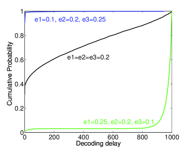
Figure 2: CDF for the upper bound on the decoding delay of receiver $R_{1}$ for the proposed random walk model based on 10000 simulations with 1000 slots for three different cases of erasure probabilities.

Any effort to control the delay by means of informed coding decisions amounts to creating opportunities for non-leading nodes to achieve the leader status. In our random walk interpretation, this is equivalent to pushing the target receiver to the first quadrant, whenever it has spent more than an acceptable amount of time in the other three quadrants. From a mathematical point of view, changing the encoding rule corresponds to altering the probabilities assigned to each direction of the random walk, thus making trajectories towards the first quadrant more likely. Achieving this goal in practice is the topic of the next section.

IV Online Network Coding with Delay Constraints

In the following, we present online network coding algorithms that are targeted towards effective delay control. The underlying system setup is the one we described in Section II.

IV-A Systematic Online Network Coding

As argued in the previous section, the desirable properties of ANC in terms of throughput optimality and a small sender queue size come at the expense of a potentially high decoding delay. We will now show that by allowing for some flexibility with respect to the sender’s queue size, we can significantly reduce the average delay — without sacrificing throughput.

Systematic Online Network Coding (SNC): A packet that is transmitted by the sender for the first time, is sent uncoded. Whenever the current leader suffers a packet loss, the next packet transmitted by the sender is a linear combination containing the last unseen packet of each receiver.

An example of the SNC algorithm is given in Table IV. It is not difficult to see that SNC does quite the opposite of ANC, in the sense that the packets sent after receiver 2 loses a packet remain uncoded, whereas ANC enforces their encoding. Conversely, a packet loss at receiver 1 causes the transmission of the coded packet ${\bf p_{1}}\oplus{\bf p_{7}}$ in time slot 8, whereas in the case of ANC the same event causes the transmissions of an uncoded packet.

The average queue size at the sender increases to $\Omega((1-\epsilon)^{-2})$, the same as for traditional random linear networking coding over all packets in the sender’s queue [10], since, for the algorithm to guarantee reliable communication, packets can only be removed from the sender’s queue after they have been successfully decoded at all receivers.

TABLE IV: Example of Systematic Online Network Coding

Time Slot	Sent Packet	Receiver 1	Receiver 2
1	${\bf p_{1}}$	OK	$E$
2	${\bf p_{2}}$	OK	OK
3	${\bf p_{3}}$	OK	OK
4	${\bf p_{4}}$	OK	OK
5	${\bf p_{5}}$	OK	$E$
6	${\bf p_{6}}$	OK	OK
7	${\bf p_{7}}$	$E$	OK
8	${\bf p_{1}}\oplus{\bf p_{7}}$	OK	OK
9	${\bf p_{8}}$	OK	OK
10	${\bf p_{9}}$	E	OK
11	${\bf p_{5}}\oplus{\bf p_{9}}$	OK	E
12	${\bf p_{10}}$	OK	OK

Proposition 4

With SNC, each received packet is innovative and the algorithm is thus throughput optimal.

Proof:

A packet is sent uncoded only if it was never transmitted previously. Such a packet is clearly innovative for each receiver that obtains it. Coded packets are combinations of the oldest unseen packets of all receivers, as in ANC. Their reception thus causes a receiver to see the oldest unseen packet, which corresponds to an increase of the dimension of the information subspace available at that receiver. The proof follows analogously to the proof of throughput optimality for ANC in Theorem 3 of [10]. ∎

Since most of the packets are sent uncoded, the average packet delay is much smaller than with ANC. For the same reason, the number of required encoding and decoding operations is vastly reduced compared to ANC. In short, the SNC algorithm builds up chains over missing packets, not over all of the packets that follow a packet loss.

For real-time traffic, achieving throughput optimality is usually not possible, since packets cease to be useful to the application if they are delivered only after a certain deadline. In such a case, the sender has to give up on those packets. In this case, for SNC, only the missing packet is skipped, and, whenever possible, the sender continues to try to repair other missing packets within their deadline. ANC, on the other hand, loses the whole chain, which leads to a substantial reduction in throughput.

IV-B Online Network Coding with a Delay Threshold

To further reduce the worst-case delay for each receiver, we can trade off some of the throughput for a substantial reduction in delay. As a simple first measure to reduce delay, we can retransmit a packet in uncoded form, in case a packet deadline is in danger of being violated.

Systematic Online Network Coding with a Delay Threshold (SNCT): Let $t$ be the current time slot and $t^{i}_{j}$ be the deadline for packet ${\bf p_{j}}$ at receiver $i$. The sender proceeds as before, as long as $t<t^{i}_{j}-\delta$ for all undecoded packets $j$ and for each receiver $i$. In case a deadline for an undecoded packet $j$ is “in danger” and $t\geq t^{i}_{j}-\delta$, packet ${\bf p_{j}}$ is sent uncoded. In case receiver $i$ loses packet ${\bf p_{j}}$, this packet is repeated until the packet is either received or the deadline expires. In case multiple deadlines are in danger, the sender randomly picks a suitable undecoded packet and sends it in uncoded form.

The same concept can be applied to ANC to obtain ANC with a Delay Threshold (ANCT). Again, the sender proceeds as with ANC, as long as no deadlines for yet undecoded packets are in danger, and otherwise transmits the corresponding packet in uncoded form. Once the packet is repaired or the deadline expires, the sender resumes with transmitting combinations of the last unseen packets of all receivers. Note that in this case, it is no longer possible for an ANCT sender to discard packets once they are seen by all senders. Consequently, the expected queue size for ANC also increases to $\Omega((1-\epsilon)^{-2})$, the same as SNC and SNCT.

V Simulation Results

We investigate the performance of the different algorithms and the impact of imposing decoding deadlines by means of simulation. We use a custom simulator with a full implementation of ARQ for network coding without and with delay threshold (ANC, ANCT), as well as systematic online network coding (SNC, SNCT). Packets are broadcast by the sender and, as before, we use a simple channel model with independent erasures for the different receivers. For all simulations, the sender has 100 original packets to transmit to the receivers. The metrics we consider are the mean and worst-case decoding delay, per receiver throughput, and average and maximum queue size for the coding at the sender, averaged over multiple simulation runs. The throughput is calculated as the total number of packets decoded, divided by the number of time slots it took until the last packet was decoded.

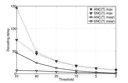
(a) Maximum and average decoding delay

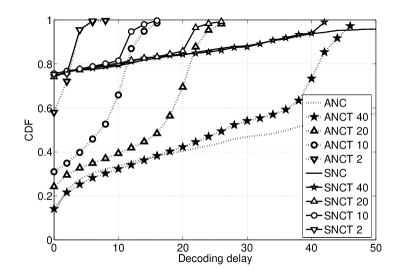
(b) CDF of decoding delay

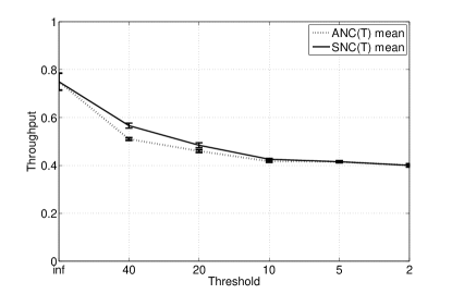
(c) Average as well as minimum and maximum throughput

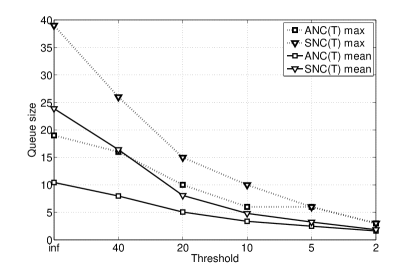
(d) Maximum and average sender queue size

Figure 3: Analysis of different delay thresholds ($\infty,40,20,10,5,2$) for 8 receivers and $\epsilon=0.25$

V-A Impact of the Delay Threshold

The value of the delay threshold is the main parameter that allows to trade off throughput for delay. Low delay thresholds increase fairness, since the difference in terms of number of received packets between the leaders and other receivers is reduced. They also reduce sender queue size for the same reason. For the simulations, we use a receiver set size of $N=8$ and the channels to the receivers all have erasure probability $\epsilon=0.25$. The sender continues to send packets according to the respective algorithms, until all receivers are able to decode all packets.

Figure 3(a) shows the maximum and the mean decoding delay for ANC and SNC without delay threshold (inf.) and for thresholds between 2 and 40. Despite the same erasure probability for all receivers, the worst case delay for ANC is close to duration of the simulation, i.e., the worst receiver has a single chain which is not broken until the very end. SNC fares much better with a worst case delay only half as large. Since with 8 receivers, ANC transmissions are usually combinations of 8 packets, a single chain may have many packets missing (not just a single one as in the two receiver case). While the oldest unseen packet that started the chain is seen with ANC at the same time as it is seen with SNC, SNC can decode that packet earlier than ANC is able to break the full chain.

The distribution of delay for all receivers is shown in Figure 3(b). For SNC(T), 75% of the packets are received without delay. The higher the threshold, the later the CDF curve jumps to a cumulative probability of 1, with the highest delay for plain SNC, reaching 1 for a delay of  75. ANC(T) has a much more varied distributions of delays, with less than a third of the packets received without delay in most cases.

Mean throughput is given in Figure 3(c), and the error bars indicate maximum and minimum throughput among the receivers. Optimum throughput is at 0.75 for ANC and SNC without threshold. (Note that the throughput of a receiver with erasure probability $\epsilon_{i}$ will be less than $1-\epsilon_{i}$ w.h.p.) The throughput reduction caused by the threshold is on the order of 30% to 40%, depending on the delay threshold chosen. As we decrease the threshold and enforce lower delays, we can also see how maximum and minimum throughput get closer and closer, leading to higher throughput fairness among the receivers. Throughput is very close for both ANC and SNC; however, SNC achieves a slightly more homogeneous distribution of throughput and thus better fairness.

Also queue size decreases when a threshold is introduced, as shown in Figure 3(d). As expected, SNC requires a larger sender queue size than ANC. However, the introduction of a threshold keeps the maximum queue size to levels that are small enough to be easily manageable at a sender, even for larger batches of packets to be sent. Overall, the benefits in terms of delay improvements outweigh the queue size increment for most realistic application scenarios.

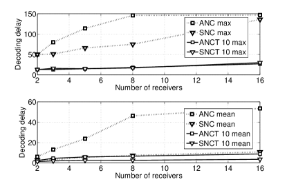
(a) Maximum delay (top) and average delay (bottom)

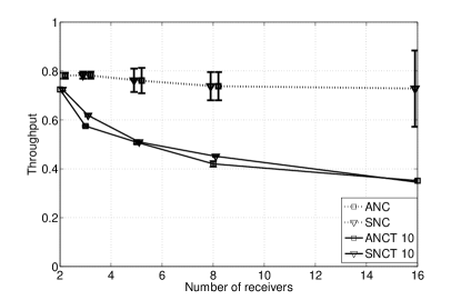
(b) Average as well as minimum and maximum throughput

Figure 4: Analysis of different sizes of receiver sets from 2 to 16 for thresholds $\infty$ and 10, and $\epsilon=0.25$

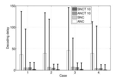
(a) Maximum delay (line) and average delay (bar)

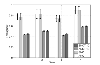
(b) Average (bar) as well as minimum and maximum throughput (line)

Figure 5: Analysis of four different cases of heterogeneous (1,2) and homogeneous (3,4) erasure probabilities for thresholds $\infty$ and 10, and for 8 receivers

V-B Impact of the Size of the Receiver Set

As the number of receivers increases, their heterogeneity in terms of number of received packets will increase as well, even if they all have the same channel erasure probability. Furthermore, as discussed in Section III, also the probability that non-leaders can decode early becomes very small. The top graph in Figure 4(a) shows that the maximum decoding delay for ANC quickly approaches the duration of the simulation of  150 time slots. While SNC has a similar worst case delay for very small and very large receiver sets, delays for intermediate sizes are significantly lower. For two receivers, chains with ANC are only missing a single packet which is repaired at the same time, as the packet is repaired through a coded transmission with SNC. Similarly, for large receiver sets, decoding the coded repair packet with SNC becomes as hard as obtaining enough degrees of freedom to decode a full chain. Introducing a delay threshold clearly lowers the worst case delay for both ANC and SNC. With a threshold of 10, packets are delivered at the latest after around 20 slots, due to multiple packets that need to be repaired at the same time, and loss of uncoded repair packets.

More importantly, for ANC the average delay even exceeds 50 time slots. Given that packets originate over the course of the simulation, the worst possible average delay is 75. This indicates that the vast majority of packets for most of the receivers can only be decoded at the end of the simulation and intermediate decoding is rare. Average delay for SNC is comparable to the average delay for ANCT with a threshold, while the average delay for SNCT is negligible.

As expected, throughput for ANC and SNC, as well as ANCT and SNCT is comparable. However, the very short delay threshold of only 10 as used in these simulations has quite a significant impact on throughput. For algorithms with delay threshold, throughput may drop down to around $\frac{1}{2}$ of that without threshold.

V-C Impact of the Erasure Probabilities

We finally evaluate algorithm performance for four different homogeneous and heterogeneous sets of erasure probabilities. The first case has 7 receivers with erasure probability 0.25, and a single receiver with erasure probability 0.15. The second case has evenly distributed erasure probabilities, with two receivers at erasure probability 0.25, two receivers at 0.2, two receivers at 0.15, and two receivers at 0.1. For the homogeneous cases, for all receivers we use an erasure probability of 0.25 in case 3 and of 0.1 in case 4. As before, there are 8 receivers and a delay threshold of 10 for ANCT and SNCT.

Since for 8 receivers even the homogeneous case shows a worst case delay close to the overall duration of the simulation, heterogeneous erasure probabilities cannot exacerbate the performance, as can be seen from Figure 5(a). For smaller sizes of receiver sets and for higher numbers of transmitted packets, intermediate decoding occurs more frequently and a much more significant advantage for the use of delay thresholds in terms of maximum decoding delay can be observed. Again, we see a throughput reduction caused by the use of delay thresholds of around 40%, as shown in Figure 5(b). However, it is important to note that if packets do become useless after their deadline expires and are discarded by the receivers, the throughput reduction caused by deadline violations is larger than that caused by the use of a delay threshold.

VI Imperfect or Delayed Feedback

So far, we assumed that the source always has perfect knowledge of the decoding status of each receiver, which is usually not feasible in practice. The overhead incurred by continuous feedback from all the receivers may be too high. Furthermore, the feedback channel may experience erasures, bit errors, and delay.

Consider the case where the feedback packet of a certain receiver is lost. When performing the next coding decision, the source does not know whether that receiver has received the previously sent packet or not. In this situation, the source can 1) assume that the receiver received that packet and now requires the next unseen packet, 2) assume that the receiver missed the packet and still requires the unseen packet reported previously, 3) perform a random experiment to decide whether to consider the packet as received or lost, or 4) ignore the receiver and not include any of its unseen packets in the coding decisions until feedback from the receiver is heard again.

The tradeoff between throughput and delay is reflected also in the treatment of missing feedback. In principle, the more optimistic the sender is in its assumptions about packet reception, the higher the expected throughput for the receivers, but the higher the risk of increased chain lengths (and thus delay). With the systematic encoding algorithms, the main event that needs to be detected is packet loss at the leader which allows to send coded repair packets. Whenever this event is detected late due to feedback loss, the same coded packet can be sent, but the delay of the repaired packets increases by the corresponding amount. Whenever the event is declared erroneously, throughput for the leader decreases since a non-innovative packet is sent but other receivers may decode a previously lost packet earlier. These considerations are also confirmed by preliminary simulations with our algorithms. Thus, the algorithms need continuous feedback from the leader, but they can easily be modified to have less frequent feedback from other receivers to reduce control overhead. Outdated information for the other receivers is often unproblematic, since only the oldest unseen packet is repaired. To this end, feedback about multiple packets can be aggregated in a feedback vector [1]. Distributed algorithms to effectively limit the amount of feedback have been developed, e.g., in the context of reliable multicast [19].

VII Conclusions

Taking the decoding delay as our primary figure of merit, we analyzed how the encoding rules of online network coding with feedback affect its performance, in scenarios with homogeneous and heterogeneous erasure probabilities. By describing the information backlog of different receivers in terms of chains of undecoded packets and by mapping their relative behavior in terms of a particular class of random walks, we were able to show that without effective delay control, weaker receivers are unlikely to recover from erasures within reasonable time and that decoding success is essentially dependent on having some advantage over other receivers in terms of received packets.

This observation motivated us to re-design the encoding stage to ensure that all receivers are able to decode at least some of the packets most of the time. Surprisingly, as our extensive simulation study shows, sending a large fraction of the packets in uncoded form provides a throughput optimal solution with striking gains in terms of decoding delay. This is particularly useful for streaming applications with stringent delay requirements, in particular when the source codec is able to cope with missing packets and thus in-order delivery of all packets is not really required.

As part of our ongoing work, we intend to combine our algorithms with a state-of-the-art video codec and tune their performance to improve the perceived video quality. This approach involves some prioritization in the decision of which packets to combine, to take into account their relative importance when decoding the video stream. We also observe that sending a packet that is in danger of missing a deadline in uncoded form is only a first step towards delay optimized coding algorithms. Coding strategies that ensure immediate decoding of such packets at the lagging receiver, while providing the other time-constrained receivers with innovative linear combinations, will further improve performance. Finally, in order to design algorithms that work well in practice, the implications of imperfect feedback need to be investigated in more detail.

References

- [1] S. Katti, H. Rahul, W. Huss, D. Katabi, M. Medard, and J. Crowcroft, “XORs in the air: Practical wireless network coding,” in ACM Sigcomm, Pisa, Italy, Sep. 2006.
- [2] C. Fragouli, J.-Y. Le Boudec, and J. Widmer, “Network coding: An instant primer,” ACM Computer Communication Review, Jan. 2006.
- [3] R. Ahlswede, N. Cai, S. Li, and R. Yeung, “Network information flow,” IEEE Trans. Information Theory, vol. 46, no. 4, 2000.
- [4] R. Koetter and M. Medard, “An algebraic approach to network coding,” IEEE/ACM Trans. Networking, vol. 49, no. 11, Nov. 2003.
- [5] T. Ho, M. Medard, J. Shi, M. Effros, and D. Karger, “On randomized network coding,” 41st Annual Allerton Conference on Communication, Control, and Computing, 2003.
- [6] P. A. Chou, T. Wu, and K. Jain, “Practical network coding,” in 41st Allerton Conference on Communication, Control and Computing, Monticello, IL, US, Oct. 2003.
- [7] A. Shokrollahi, “Raptor codes,” IEEE/ACM Trans. Networking, vol. 14, pp. 2551–2567, 2006.
- [8] C. Fragouli, D. Lun, M. Medard, and P. Pakzad, “On feedback for network coding,” in CISS, Baltimore, MD, US, Mar. 2007.
- [9] L. Keller, E. Drinea, and C. Fragouli, “Online broadcasting with network coding,” in NetCod, Hong Kong, China, Jan. 2008.
- [10] J. K. Sundararajan, D. Shah, and M. Medard, “ARQ for network coding,” in IEEE ISIT 2008, Toronto, Canada, Jul. 2008.
- [11] J. Sundararajan, D. Shah, and M. Médard, “Online network coding for optimal throughput and delay–the two-receiver case,” Arxiv preprint arXiv:0806.4264, 2008.
- [12] A. Kamra, V. Misra, J. Feldman, and D. Rubenstein, “Growth Codes: Maximizing Sensor Network Data Persistence,” in ACM Sigcomm, Pisa, Italy, Sep. 2006.
- [13] D. Munaretto, J. Widmer, M. Rossi, and M. Zorzi, “Resilient Coding Algorithms for Sensor Network Data Persistence,” in EWSN, Bologna, Italy, Jan. 2008.
- [14] R. A. Costa, D. Munaretto, J. Widmer, and J. Barros, “Informed network coding for minimum decoding delay,” in IEEE MASS, Atlanta, Georgia, Sep. 2008.
- [15] M. Wang and B. Li, “R2: Random push with random network coding in live peer-to-peer streaming,” IEEE Journal on Selected Areas in Communications, vol. 25, pp. 1655–1666, December 2007.
- [16] S. Caser and H. J. Hilhorst, “Topology of the support of the two-dimensional lattice random walk,” Phys Rev Lett., vol. 77, no. 6, pp. 992–995, Aug. 1996.
- [17] J. W. Cohen, “On the random walk with zero drifts in the first quadrant of R2,” Stochastic Models, vol. 8, no. 3, pp. 359–374, 1992.
- [18] A. Asselah and P. A. Ferrari, “Hitting times for independent random walks on Zd,” Annals of Probability, vol. 34, no. 4, pp. 1296–1338, 2006.
- [19] T. Fuhrmann and J. Widmer, “On the scaling of feedback algorithms for very large multicast groups,” Special Issue of Computer Communications on Integrating Multicast into the Internet, 2001.