Stress singularities and the formation of birefringent strands in stagnation flows of dilute polymer solutions

Abstract

We consider stagnation point flow away from a wall for creeping flow of dilute polymer solutions. For a simplified flow geometry, we explicitly show that a narrow region of strong polymer extension (a birefringent strand) forms downstream of the stagnation point in the UCM model and extensions, like the FENE-P model. These strands are associated with the existence of an essential singularity in the stresses, which is induced by the fact that the stagnation point makes the convective term in the constitutive equation into a singular point. We argue that the mechanism is quite general, so that all flows that have a separatrix going away from the stagnation point exhibit some singular behaviour. These findings are the counterpart for wall stagnation points of the recently discovered singular behaviour in purely elongational flows: the underlying mechanism is the same while the different nature of the singular stress behaviour reflects the different form of the velocity expansion close to the stagnation point.

, and

1 Introduction

Extensional flows of polymer solutions and melts occur in many industrial polymer processing operations, and hence such flows have been studied for decades [1, 2]. Recently however, interest in extensional flows was renewed by observations of steady and unstable continuous flow in microfluidic devices [3, 4, 5], and it was realized only recently that extensional flows are prone to the formation of singularities and non-analytic structures in the stress fields [6, 7, 8]. Depending on the Deborah number and the model used, these stress singularities may take various forms. For purely extensional flow in continuum models that describe infinitely extensible polymer chains (such as the upper convected Maxwell model (UCM) and the Oldroyd-B model [1, 2, 9]) the stresses can have power law spatial behaviour with a finite limit at the centre line, or they even have power law divergencies. For models that are based on finitely extensible chains, divergencies are cut off at some scale, but singular behaviour of the stress gradients may persist [6, 7, 8]. Such singular behaviour may have important implications for numerical simulations of extensional flows, since it leads to structures with a very small length scale. Indeed it is known that for many such flows, numerical schemes break down at only moderate flow rates (Deborah numbers of order unity).

The question quite naturally comes up whether singular behaviour near special points is the rule rather than the exception. We argue in this Communication that the latter is the case and demonstrate this for a simplified case where all calculations can be done analytically, so that the emergence of the singular behaviour can be followed explicitly.

The reason to expect singular behaviour near special points where the velocity vanishes — even though the geometry is not singular — is actually very simple. For steady flow, the only derivative terms of the stress $\mathbf{T}$ in UCM-type constitutive equations come from the convective term $(\mathbf{v}\cdot\mathbf{\nabla})\mathbf{T}$. The points where $\mathbf{v}$ vanishes — the stagnation point in elongational flow or in the wall stagnation point flow considered here — thus translate into a singular point [10] of the partial differential equation obtained from the constitutive equation for the stress. Close to the singular point, the lowest order terms in the expansion of $\mathbf{v}$ are often fixed by simple symmetry considerations and boundary conditions, if applicable. So the nature of the dominant singularity at the singular point is generally fixed independent of the precise details of the model. Further away from the singularity, the behaviour will typically depend on the details of the flow profile. All these features are well illustrated by the analysis below. As stated, we focus on a simple case where the calculations can all be done analytically, but the scenario holds generally for complex more realistic flows and we suspect this mechanism of advection to be at the origin of the formation of birefringent strands.

We focus on wall stagnation point flows where the flow is away from the wall. Examples of this are flows in the wake of a falling sphere or of a fixed cylinder, as shown schematically in Fig. 1 (a). In particular, the flow past a fixed cylinder or sphere in a channel has become a benchmark problem for numerical modelling of viscoelastic constitutive equations [11, 12, 13]. It is known that in such flows a narrow region of high polymer extension may form, a so-called birefringent strand [14, 15]. This region starts at a small but finite distance downstream from the stagnation point, as indicated schematically in Fig. 1 (b), where a flow near a flat wall is depicted.

In this work, we consider a strictly two-dimensional version of this flow, with a simplified, fixed velocity field obeying the basic symmetry of a stagnation point at a wall (cf. [11]). We analyse this case in detail for the UCM model [1, 2, 9] but also discuss in the end the qualitative changes that occur for a FENE-P model.

Unlike the case of steady purely extensional flow, which was analysed previously [6, 7, 8], the extension of the polymers does not diverge for any extension rate. We find that a thin birefringent strand forms, with a singularity at its centre. As argued above, notwithstanding the simplifications we make in obtaining this result, we believe that the analysis makes it clear how singular behaviour emerges in general.

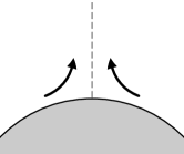
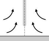
(a)	(b)

Figure 1: Stagnation flow (a) in a wake, (b) approximated by a flow near a flat wall. In (b) the formation of a birefringent strand is qualitatively indicated by the shaded area.

Unfortunately, our results cannot immediately be compared quantitatively with experiments or numerical computations on realistic cases like flow past a cylinder [12, 13]. First, one should keep in mind that in such situations, there may be two sources of (near) singular behaviour: besides the one we analysed here, dominated by the symmetry and boundary conditions of the velocity field near the wall stagnation point, in viscoelastic flow past a cylinder large stress fields are already built up at the sides of the cylinder, where the flow is mostly along the cylinder. These shear stresses are advected toward the rear stagnation point. This effect is clearly not present in the simplified geometry that we consider. Second, our analysis is based on taking a fixed velocity field obeying the basic symmetry, and we show how this leads to an essential singularity in the stress. In reality, of course, the velocity and stresses are coupled indirectly through the momentum balance equation. Through this coupling, the velocity field will also be affected in the region of large stress gradients near the stress singularity. Since the symmetry and expansion of the velocity near the stagnation point cannot change in lowest order, we expect that there is an intermediate flow regime where the basic structure of the singularity is not changed dramatically. This assumption is further supported by recent simulations of a two-dimensional cross-slot flow by Poole et al. [5]. There, the velocity profiles remained smooth even when the flow changed its symmetry (the new type of purely elastic instability discovered by Arratia et al. [4]), while stresses exhibit the typical singular structure similar to the one discussed in [6, 8]. At the same time, numerical studies suggest that at sufficiently large flow rates, this nonlinear coupling can become so strong that there may be no steady state flow solution past a cylinder for Deborah numbers of order unity [12, 16]. The coupling and this effect are, unfortunately, beyond the present approximation.

The layout of this paper is as follows. In section 2 we introduce the flow geometry and the models, and we briefly recapture similarity solutions for UCM found by other authors [17, 18]. We calculate analogous solutions for a simplified version of this flow, where we fix the velocity field, for UCM and FENE-P. In section 3 we consider more realistic boundary conditions, and we solve the constitutive equations analytically. In section 4 we consider the resulting stress field (extension field) in more detail, showing that we find a narrow region of high polymer extension, with a non-analytic stress profile at the centre of the strand. We then discuss these results in the light of more realistic flow profiles, and we conclude by discussing the relevance of these results for computational and experimental work.

2 Simplified stagnation flow of a UCM fluid

We consider incompressible planar stagnation flow of a UCM fluid without inertia (creeping flow). The UCM constitutive equation for steady flow is [1]

$$\mathbf{T}+\lambda\left[(\mathbf{v}\cdot\mathbf{\nabla})\mathbf{T}-(\mathbf{\nabla}\mathbf{v})^{T}\cdot\mathbf{T}-\mathbf{T}\cdot(\mathbf{\nabla}\mathbf{v})\right]=\eta\left(\mathbf{\nabla}\mathbf{v}+(\mathbf{\nabla}\mathbf{v})^{T}\right),$$ (1)

where $\lambda$ is the relaxation time of the fluid and $\eta$ is the Newtonian viscosity. The momentum balance for creeping flow is

$$\mathbf{\nabla}\cdot\mathbf{T}-\mathbf{\nabla}p=0,$$ (2)

where $p$ is the pressure. Incompressibility is given by

$$\mathbf{\nabla}\cdot\mathbf{v}=0.$$ (3)

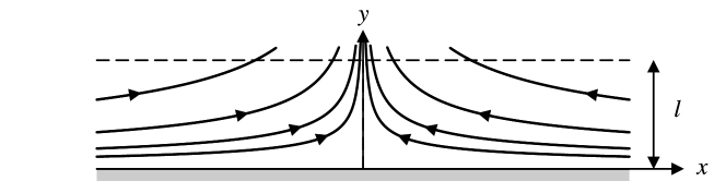
Figure 2: Planar stagnation flow.

The planar stagnation flow geometry we consider is depicted in Fig. 2. We take the vertical direction as bounded, with length $\ell$. Because of the solid wall, the boundary condition at the wall ($y=0$) is $\mathbf{v}=0$. At $y=\ell$, we impose $v_{y}=V$, with $V>0$. For the velocity field, a similarity solution then exists, which is of the form [17, 18]

$$v_{x}=-x\psi^{\prime}(y)\quad\textrm{and}\quad v_{y}=\psi(y),$$ (4)

where the boundary conditions imply $\psi(0)=0$ and $\psi^{\prime}(0)=0$. Inspired by this solution, we take a fixed velocity field that satisfies the boundary conditions and that would correspond to the lowest-order approximation near the wall:

$$v_{x}=-2(V/\ell^{2})xy\quad\textrm{and}\quad v_{y}=(V/\ell^{2})y^{2}.$$ (5)

Note that these terms are the lowest order analytic terms in an expansion in $x$ and $y$ away from a symmetric stagnation point at the wall. This is why our analysis illustrates the emergence of singular behaviour in more general cases as well.

Let us now insert this velocity field into the constitutive equation. The resulting stress field will not in general satisfy momentum balance, but it does yield a valid solution for Newtonian creeping flow. This is sometimes referred to as “Newtonian kinematics”; in the Oldroyd-B extension of the UCM model, this would be a reasonable approximation in the dilute limit, $\beta\ll 1$, in which the polymer stresses do not influence the flow [18, 16].

We can rescale the quantities appearing in the equations: length is scaled with $\ell$, velocity with $V$, and stress with $\eta V/\ell$. The velocity field becomes

$$v_{x}=-2xy\quad\textrm{and}\quad v_{y}=y^{2},$$ (6)

with $0\leq y\leq 1$, and for the constitutive equation we obtain a dimensionless form

$$\mathbf{T}+\operatorname{De}\left[(\mathbf{v}\cdot\mathbf{\nabla})\mathbf{T}-(\mathbf{\nabla}\mathbf{v})^{T}\cdot\mathbf{T}-\mathbf{T}\cdot(\mathbf{\nabla}\mathbf{v})\right]=\mathbf{\nabla}\mathbf{v}+(\mathbf{\nabla}\mathbf{v})^{T}.$$ (7)

Here we introduced the Deborah number

$$\operatorname{De}=\lambda V/\ell.$$ (8)

We can then insert the rescaled velocity into the constitutive equation and solve for the stresses. We obtain equations for the components of the stress tensor, and we observe that the equation for the $yy$ component decouples from the other equations, because $\partial v_{y}/\partial x$ is identically zero for this velocity field. The equation for the $yy$ component becomes

$$T_{yy}+\operatorname{De}\left[-2xy\frac{\partial T_{yy}}{\partial x}+y^{2}\frac{\partial T_{yy}}{\partial y}-4yT_{yy}\right]=4y.$$ (9)

Let us first analyse the solution of this equation under the often-made assumption that $T_{yy}$ is constant in $x$ [17] and then analyse why this solution misses an important part of the physics. One might naively think that this solution can be seen as the first term in a series expansion in powers of $x$ [18], but as we shall see this assumption itself is incorrect: singular terms are typically generated by the stagnation point flow. Defining

$$T_{yy}(x,y)\equiv Y(y),$$ (10)

we solve

$$Y(y)+\operatorname{De}\left[y^{2}Y^{\prime}(y)-4yY(y)\right]=4y.$$ (11)

This equation allows an exact solution, and we find

$$Y_{\textrm{gen}}(y)=4y+12\operatorname{De}y^{2}+24\operatorname{De}^{2}y^{3}+24\operatorname{De}^{3}y^{4}+Cy^{4}\exp[1/(\operatorname{De}y)],$$ (12)

where the last term corresponds to the homogeneous solution of the differential equation, and $C$ is a constant of integration. This term clearly leads to unphysical results, as it implies $|Y(y)|\to\infty$ as $y\to 0^{+}$. Hence, if one thinks of $Y(y)$ as the first term in a regular series expansion in $x$, we should discard it and keep only the particular solution

$$Y_{0}(y)=4y+12\operatorname{De}y^{2}+24\operatorname{De}^{2}y^{3}+24\operatorname{De}^{3}y^{4}.$$ (13)

A few remarks about this solution are in order: (i) It does not in general satisfy momentum balance, but it is qualitatively similar to the more accurate similarity solution of Öztekin et al. [18]. (ii) By forcing the solution to be independent of $x$, we find a solution that can only be seen as an approximation that is valid in a small range around $x=0$. (iii) We assume the same functional form of the velocity field for all $\operatorname{De}$. (iv) The solution does not diverge at finite $y$ for any $\operatorname{De}$. This is in contrast with purely extensional flow, where stresses diverge for $\operatorname{De}\geq 1/2$.

Let us now discuss the shortcoming of the above line of analysis. The solution is an admissible solution if we work in the infinite domain $x\to\pm\infty$. However, if we work in a finite domain, with boundary conditions at some finite $x=\pm L$, say, then the solution is only relevant if the stresses on this boundary are precisely consistent with (13). In general, the boundary stresses are incompatible with this expression and the flow drawn in Fig. 2 advects all deviations from this expression towards the stagnation point. While in the above analysis it appears as if the analysis close to the stagnation point dictates what the proper boundary condition far to the left and right should be, in reality we have to analyse what happens with the stresses as they are advected from the left and right to the stagnation point. That dictates the behaviour there, not the other way around! The analysis below does show that singular behaviour is picked up through this advection from the boundaries, as one might expect.

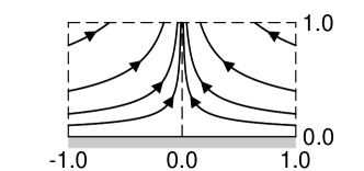
Figure 3: Planar stagnation flow on the finite rectangular domain analysed in this paper.

3 Inflow boundary conditions and an explicit solution

To back up the above observations, we now allow explicit $x$-dependence of the stress field without including higher orders in $x$ in the velocity field. We can then match more realistic inflow boundary conditions by including homogeneous parts of the solution, and we shall see that this causes qualitative changes in the stress field.

To do so, we modify the geometry by explicitly taking a finite domain in the $x$ direction, with $-1\leq x\leq 1$, see Fig. 3. We observe that the equation is purely advective. This implies that is it a first-order differential equation and that there is no “interaction” across streamlines. We can therefore split the domain in two separate parts, one for $x<0$ and one for $x>0$, with the line $x=0$ acting as the separatrix between the two domains. As in the case of pure extensional flow, this allows for non-analyticity on the line $x=0$. [6, 7, 8]. On each of the two subdomains, we can impose independent inflow boundary conditions. We will restrict ourselves to the domain $0\leq x\leq 1$, and we will assume that the negative domain is the mirror image of this domain. On the lateral boundary $x=+1$ we impose the boundary condition $T_{yy}(x=1,y)=Y_{\textrm{b}}(y)$ with $Y_{\textrm{b}}(0)=0$.

We thus consider again the differential equation (9):

$$Y(x,y)+\operatorname{De}\left[-2xy\frac{\partial Y(x,y)}{\partial x}+y^{2}\frac{\partial Y(x,y)}{\partial y}-4yY(x,y)\right]=4y.$$ (14)

In the language of local analysis of differential equations, this partial differential equation has an irregular singular point at $x=y=0$ [10].

It is easy to check that the partial differential terms in the equation together give identically zero if $Y$ is a function of $xy^{2}$ only. In other words, the form

$$Y(x,y)\equiv f(xy^{2}),$$ (15)

is a zero mode of the differential operator since

$$-2xy\frac{\partial f(xy^{2})}{\partial x}+y^{2}\frac{\partial f(xy^{2})}{\partial y}\equiv 0$$ (16)

for any function $f$.

Now, due to the linearity of the equation, the solution of the equation is the sum of the particular solution $Y_{0}$ given in (13) plus an arbitrary solution $Y_{\textrm{hom}}(x,y)$ of the homogeneous equation, that is

$$Y(x,y)=Y_{0}(y)+Y_{\textrm{hom}}(x,y).$$ (17)

Moreover, if we assume $Y_{\textrm{hom}}$ to be of the form

$$Y_{\textrm{hom}}(x,y)=g(y)h(xy^{2}),$$ (18)

then inserting this into the homogeneous part of the equation (with right hand side equal to zero) effectively gives an equation for $g(y)$ that is identical to the homogeneous part of Eq. (11). For $g$ we thus recover the homogeneous solution of (11), that is, the last term of (12). Thus, we have

$$Y(x,y)=Y_{0}(y)+y^{4}\exp[1/(\operatorname{De}y)]h(xy^{2})$$ (19)

We can now impose the boundary condition $Y(x=1,y)=Y_{\textrm{b}}(y)$ at $x=1$: requiring that $Y(x=1,y)$ given by (19) equals $Y_{\textrm{b}}(y)$, immediately gives

$$h(y^{2})=\frac{Y_{\textrm{b}}(y)-Y_{0}(y)}{y^{4}}\,\exp[-1/(\operatorname{De}y)].$$ (20)

Since $h(xy^{2})$ is a function of the product $xy^{2}$ only, we now know $h$ for all $x$ and $y$. This finally gives the general full solution

$$Y(x,y)=Y_{0}(y)+\frac{Y_{\textrm{b}}\left(\sqrt{xy^{2}}\right)-Y_{0}\left(\sqrt{xy^{2}}\right)}{x^{2}}\,\exp\left[\frac{1-1/\sqrt{x}}{\operatorname{De}y}\right].$$ (21)

Note that the structure is precisely as we envisioned: the deviations of the $x$-independent solution $Y_{0}(y)$ from the stress boundary condition $Y_{\textrm{b}}(y)$ are convected towards the stagnation point, and the stresses there are largely dominated by the singularity.

For the flow that we consider, we use the procedure above to match the stress field to the inflow boundary condition. For simplicity we take this to be

$$Y_{b}(y)\equiv 0,$$ (22)

but since the behaviour for small $x$ is dominated by the singular term, other choices lead to similar conclusions. For $\operatorname{De}=1$ we then find the stress field in Fig. 4. Since we consider the ultradilute limit, one may also think of this as the polymer extension in the $yy$ direction (see below).

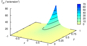
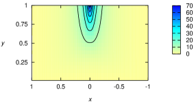
(a)	(b)	(c)

Figure 4: Polymer extension in a simplified wall stagnation flow for ultradilute UCM fluid, for $\operatorname{De}=1.0$: (a) three-dimensional plot of the extension as a function of $x$ and $y$, (b) contour plot of the extension, showing the shape of the birefringent strand, (c) cross-section of the extension profile for $y=0.25,0.5,0.75,1.0$

We clearly see that a narrow region of high extensional stress (polymer extension) forms in the centre of the domain. The solution we find does not diverge for any $\operatorname{De}$, nor does any gradient diverge — in fact, the $x$-derivatives are zero to any order on the centre line, and we have an essential singularity there.

4 Distance from the wall

The stress profile $Y_{0}(y)$, Eq. (13), for a UCM fluid has no intrinsic length scale, as the UCM model has no characteristic stress or extension. Therefore, we cannot obtain a meaningful “distance from the wall” in that model. Models with finite extensibility, such as the well-known FENE-P model, are required to do this. In previous work we argued [8] that for extensional flow a fair approximation to the FENE-P model can be obtained by restricting to the $yy$ extensional component of the stress tensor, and making the simple approximation that the polymer stretching follows the UCM rheology up to a certain maximum extensional stress after which the stress does not increase any further (this is sometimes referred to as a linear-locked approximation [19, 20]). This maximal stress should correspond to the maximal extension $L$ in the FENE-P model, for which the trace of the conformation tensor $\mathbf{A}$ is $L^{2}$. The UCM stress tensor is related to the FENE-P conformation tensor as $\mathbf{A}=\mathbf{1}+\operatorname{De}\mathbf{T}$ (this can be seen by taking $L\to\infty$ in the FENE-P constitutive equations, and comparing this to the UCM constitutive equations). Restricting to the $yy$ component, we find $1+\operatorname{De}T_{yy}^{\textrm{max}}=L^{2}$. In Fig. 5 we show stress profiles for the simplified velocity field, for the UCM model and a FENE-P-like model that is restricted to the $yy$ component.

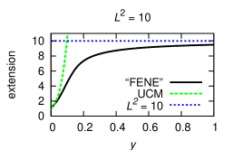
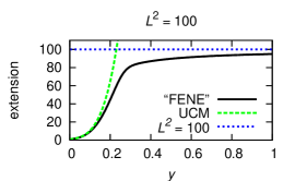
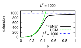
Figure 5: Polymer extension in a simplified wall stagnation flow for ultradilute FENE-P fluid, for $\operatorname{De}=5.0$, and $L^{2}=10.0,100.0,1000.0$.

In this approximation and for a fixed velocity field, we can thus estimate the distance of the strand from the wall, as well as the width of the strand, by considering the locus of points where the UCM extension $1+\operatorname{De}T_{yy}$ reaches $L^{2}$. For our fixed velocity field, it is straightforward to find scaling relations for the distance and the width as functions of $\operatorname{De}$ and $L^{2}$. From Eq. (13) we see that the distance $y_{0}$ from the wall is given in our approximation by

$$1+\operatorname{De}y_{0}+12\operatorname{De}^{2}y_{0}^{2}+24\operatorname{De}^{3}y_{0}^{3}+24\operatorname{De}^{4}y_{0}^{4}=L^{2}.$$ (23)

This means that $y_{0}$ scales as $1/\operatorname{De}$ for fixed $L^{2}\gg 1$ and all $\operatorname{De}$. For fixed $\operatorname{De}$ we find that $y_{0}$ should scale as $(L^{2})^{1/4}=\sqrt{L}$ for $L^{2}\to\infty$. We conclude that

$$y_{0}=\frac{\sqrt{L}}{\operatorname{De}}\frac{1}{24^{1/4}}f(L^{2})\quad\textrm{with}\quad f(L^{2})<1\textrm{ and }f(L^{2}\to\infty)=1.$$ (24)

This asymptotic result cannot be easily extended to other, more realistic velocity fields. Note that in the limit of large $L^{2}$, the distance $y_{0}$ will become larger than $1$, and it falls outside the domain that we assumed, $0\leq y\leq 1$. The general conclusion that the distance increases with $L^{2}$ and decreases with $\operatorname{De}$ is of course physically reasonable: for larger $L^{2}$ at fixed $\operatorname{De}$ it takes a longer distance to fully stretch the polymers, while for larger $\operatorname{De}$ at given $L^{2}$, the stretching occurs more rapidly and one may expect that the distance required for full stretching decreases, at least on the centre line of the flow.

5 Width of the strand

The width of the strand is a more subtle issue. Since the stress is bounded, and therefore also the UCM extension, we can define a meaningful length scale even in the UCM model, as can be seen from the left panel of Fig. 6. For example, we can take the full width at half maximum (FWHM) of the peak. In that case, the width decreases as a function of $\operatorname{De}$. We can also look at our FENE-P-like approximation and use the contour line where the profile reaches a given $L^{2}$. A numerical analysis shows that the FWHM decreases as $1/\operatorname{De}^{2}$, while the approximate FENE-P width increases monotonically and saturates, see the right panel of Fig. 6.

These asymptotic results can be explained from the exact solution, Eq. (21). The FWHM is mostly determined by the behaviour close to the centre of the strand, where the factor $\exp[-1/(\operatorname{De}\sqrt{x})]$ dominates: as $x\to 0$ it vanishes more rapidly than the factors in front of it diverge. The typical length scale $x_{0}$ for this exponential factor is given by $\sqrt{x_{0}}\operatorname{De}\sim 1$, or $x_{0}\propto 1/\operatorname{De}^{2}$, and thus, the FWHM also scales as $1/\operatorname{De}^{2}$. For the FENE-P-like width we make the observation that the UCM extension as a function of $x$ actually converges pointwise as $\operatorname{De}\to\infty$:

$$\lim_{\operatorname{De}\to\infty}\left(1+\operatorname{De}Y(x,y)\right)=\frac{1}{x^{2}}\quad\textrm{(pointwise in $x$).}$$ (25)

It is then evident that for given $L^{2}$, the width will approach a constant value of $2/L^{2}$ for $\operatorname{De}\to\infty$.

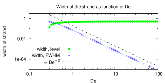
Figure 6: The left panel shows the cross-section of the “UCM extension” profile at $y=1.0$ for a range of Deborah numbers, $\operatorname{De}=0.30,0.55,1.00,1.81,3.31,6.03$. The right panel shows a log-log plot of the width of the peak, both as a FWHM measure and for a FENE-P-like definition (see text).

6 Discussion

One may ask the question to what extent the analysis above is relevant for “real” flow profiles. We already argued above that although the details may (and will) change, the qualitative behaviour (localization of the extensional stress along the separatrix and non-analyticity) will persist.

The procedure that was performed to obtain the stress profile can be repeated for the “exact” velocity field in Refs. [17] and [18], using numerical integration where necessary. That would still yield a solution that does not obey the momentum balance equation (2), but more importantly, it would not qualitatively change the singularity that we find. Mathematically, this happens as follows. In the region near the stagnation point $x=y=0$, the velocity field is expected to have, in lowest order, always terms like in (5). Hence, in this regime, the equation always has “zero mode” solutions $f(xy^{2})$ of the convective part of the constitutive equation. Only in special cases will this term not be excited. Furthermore, close to the wall, the dominant behaviour of the $y$-independent homogeneous solution must go as $\exp[-1/(\operatorname{De}y)]$ and this then has to be compensated by a similar essential singularity in $\sqrt{x}y$. Thus, close to the wall this essentially singular behaviour is robust. Further away from the wall, however, the behaviour will change if the velocity field crosses over to a different $y$-dependence.

Similar considerations apply to other modifications that are used to give a more realistic description within the UCM framework. As long as the velocity field is reasonably well-behaved, the extension profile on the separatrix is determined only by the velocity on the separatrix.

In fact, we see that the only ingredients that we need in order to obtain our results, are the general form of the velocity field Eq. (4), the “advective” part of the constitutive equation, as in Eq. (16), and the absence of a stress diffusion term in the constitutive equation. This strongly suggests that both the localization and the nonanalytic behaviour at $x=0$ depend on these ingredients and not so much on the particular form of the constitutive equations. One would then expect that every viscoelastic flow with a stagnation point gives rise to singular behaviour downstream of the stagnation point.

We already mentioned that the stress profile we obtained does not satisfy the Navier-Stokes equation (momentum balance). It would be interesting to see how we might modify the velocity profile to have the system obey the Navier-Stokes equation. It is difficult to do this analytically, but given the singular structure of the stress field, it is to be expected that a correction to the velocity field will show a similar singularity for intermediate flow rates. As we mentioned in the introduction, for sufficiently large flow rates, this coupling may cause a breakdown of the steady state flow solution [12, 13].

7 Conclusions

Not only purely extensional flow but also (reverse) wall stagnation flow shows strong localization of extensional stresses and non-analytic behaviour. At moderate and high Deborah numers, a birefringent strand is formed, with an essential singularity at its centre. The polymer extension becomes appreciable at a finite distance from the wall, and the width of the strand either decreases or becomes constant with increasing Deborah number, depending on the definition. Asymptotic scaling relations can be found for both the distance from the wall and the strand width. Although concrete numerical and analytical results have been calculated only for a fixed velocity field, the qualitative behaviour that we find should carry over to more realistic flows, at least if the usual constitutive equations are to be taken seriously. If an artificial stress diffusion term is added to the constitutive equation, as is sometimes done in numerical simulations to enhance stability, the mathematical singularity will disappear. Nevertheless, the behaviour we have analysed here should still dominate most of the profiles if the diffusion constant takes on any value that is physically reasonable.

We suggest that the localization and the singular behaviour are caused by the purely advective character (without diffusion) of the constitutive equation, combined with the extensional character of the flow. We further suggest that the occurrence of this behaviour does not depend on the exact formulation of the constitutive equations, as long as these include stress advection and stress relaxation. The non-analyticity at the separatrix is a result of the absence of diffusion, which essentially decouples the domains on either side of the separatrix.

As we noted in the introduction, internal stagnation point flows were recently shown to exhibit singular behaviour of the type $|y|^{\beta}$, where $y$ is the upstream distance from the singular line. Such singularities may easily cause numerical problems since derivatives of sufficiently high order diverge. In the case of wall stagnation flow, the situation may at first sight not be as bad for numerical approaches, since all derivatives remain finite. Nevertheless, for large Deborah numbers there is a rapid crossover region, the width of which decreases as $1/\operatorname{De}^{2}$ for large $\operatorname{De}$. This region will have to be resolved numerically.

References

- [1] R. B. Bird, C. F. Curtiss, R. C. Armstrong, O. Hassager, Dynamics of polymeric liquids, 2nd Edition, Vol. 1. Fluid Mechanics, Wiley, New York, 1987.
- [2] R. B. Bird, C. F. Curtiss, R. C. Armstrong, O. Hassager, Dynamics of polymeric liquids, 2nd Edition, Vol. 2. Kinetic theory, Wiley, New York, 1987.
- [3] L. Xi, M. D. Graham, A mechanism for oscillatory instability in viscoelastic cross-slot flow, J. Fluid Mech., in press. arXiv:physics/0703262 (2007).
- [4] P. E. Arratia, C. C. Thomas, J. Diorio, J. P. Gollub, Elastic instabilities of polymer solutions in cross-channel flow, Phys. Rev. Lett. 96 (2006) 144502.
- [5] R. J. Poole, M. A. Alves, P. J. Oliveira, Purely elastic flow asymmetries, Phys. Rev. Lett. 99 (2007) 164503.
- [6] M. Renardy, A comment on smoothness of viscoelastic stresses, J. Non-Newtonian Fluid Mech. 138 (2006) 204–205.
- [7] B. Thomases, M. Shelley, Emergence of singular structures in Oldroyd-B fluids, Phys. Fluids 19 (2007) 103103.
- [8] P. Becherer, A. N. Morozov, W. van Saarloos, Scaling of singular structures in extensional flow of dilute polymer solutions, J. Non-Newtonian Fluid Mech. 153 (2008) 183–190.
- [9] R. G. Larson, The Structure and Rheology of Complex Fluids, Oxford University Press, Oxford, 1999.
- [10] C. M. Bender, S. A. Orszag, Advanced mathematical methods for scientists and engineers, McGraw-Hill, New York, 1978.
- [11] P. Wapperom, M. Renardy, Numerical prediction of the boundary layers in the flow around a cylinder using a fixed velocity field, J. Non-Newtonian Fluid Mech. 125 (2005) 35–48.
- [12] Y. Fan, H. Yang, R. I. Tanner, Stress boundary layers in the viscoelastic flow past a cylinder in a channel: limiting solutions, Acta Mech. Sinica 21 (2005) 311–321.
- [13] M. A. Hulsen, R. Fattal, R. Kupferman, Flow of viscoelastic fluids past a cylinder at high Weissenberg number: stabilized solutions, J. Non-Newtonian Fluid Mech. 127 (2005) 27–39.
- [14] R. Cressely, R. Hocquart, Birefringence d’écoulement localisée induite à l’arrière d’obstacles, Optica Acta 27 (1980) 699–711.
- [15] O. G. Harlen, J. M. Rallison, M. D. Chilcott, High-Deborah-number flow of a dilute polymer solution past a sphere falling along the axis of a cylindrical tube, J. Non-Newtonian Fluid Mech. 33 (1990) 157–173.
- [16] M. Bajaj, M. Pasquali, J. Ravi Prakash, Coil-stretch transition and the breakdown of computations for viscoelastic fluid flow around a confined cylinder, J. Rheol. 52 (2008) 197–223.
- [17] N. Phan-Thien, Plane and axi-symmetric stagnation flow of a Maxwellian fluid, Rheol. Acta 22 (1983) 127–130.
- [18] A. Öztekin, B. Alakus, G. H. McKinley, Stability of planar stagnation flow of a highly viscoelastic fluid, J. Non-Newtonian Fluid Mech. 72 (1997) 1–29.
- [19] O. J. Harris, J. M. Rallison, Start-up of a strongly extensional flow of a dilute polymer solution, J. Non-Newtonian Fluid Mech. 50 (1993) 89–124.
- [20] O. J. Harris, J. M. Rallison, Instabilities of a stagnation point flow of a dilute polymer solution, J. Non-Newtonian Fluid Mech. 55 (1994) 59–90.