Efficiency of Magnetic to Kinetic Energy Conversion in a Monopole Magnetosphere

Abstract

Unconfined relativistic outflows from rotating, magnetized compact objects are often well-modeled by assuming the field geometry is approximately a split-monopole at large radii. Earlier work has indicated that such an unconfined flow has an inefficient conversion of magnetic energy to kinetic energy. This has led to the conclusion that ideal magnetohydrodynamical (MHD) processes fail to explain observations of, e.g., the Crab pulsar wind at large radii where energy conversion appears efficient. In addition, as a model for astrophysical jets, the monopole field geometry has been abandoned in favor of externally confined jets since the latter appeared to be generically more efficient jet accelerators. We perform time-dependent axisymmetric relativistic MHD simulations in order to find steady state solutions for a wind from a compact object endowed with a monopole field geometry. Our simulations follow the outflow for $10$ orders of magnitude in distance from the compact object, which is large enough to study both the initial “acceleration zone” of the magnetized wind as well as the asymptotic “coasting zone.” We obtain the surprising result that acceleration is actually efficient in the polar region, which develops a jet despite not being confined by an external medium. Our models contain jets that have sufficient energy to account for moderately energetic long and short gamma-ray burst (GRB) events ($\sim 10^{51}$–$10^{52}$ erg), collimate into narrow opening angles (opening half-angle $\theta_{j}\approx 0.03$ rad), become matter-dominated at large radii (electromagnetic energy flux per unit matter energy flux $\sigma<1$), and move at ultrarelativistic Lorentz factors ($\gamma_{j}\sim 200$ for our fiducial model). The simulated jets have $\gamma_{j}\theta_{j}\sim 5$–$15$, so they are in principle capable of generating “achromatic jet breaks” in GRB afterglow light curves. By defining a “causality surface” beyond which the jet cannot communicate with a generalized “magnetic nozzle” near the axis of rotation, we obtain approximate analytical solutions for the Lorentz factor that fit the numerical solutions well. This allows us to extend our results to monopole wind models with arbitrary magnetization. Overall, our results demonstrate that the production of ultrarelativistic jets is a more robust process than previously thought.

1. Introduction

Gamma-ray bursts (GRBs), active galactic nuclei (AGN), x-ray binaries, and pulsar wind nebulae (PWNe) are among the most powerful systems in the Universe. Their power originates from a central engine that contains a rotating, magnetized compact object such as a neutron star or black hole (Goldreich & Julian, 1969; Blandford & Znajek, 1977) or from a surrounding accretion disk (Shakura & Sunyaev, 1973; Novikov & Thorne, 1973; Lovelace, 1976). These systems obtain their angular momentum and strong magnetic field from their environment either by advection during their formation or through accretion which is known to amplify any weak field by magnetorotational turbulence (Balbus & Hawley, 1998). The region around the compact object is often expected to contain a highly-magnetized dipolar magnetosphere that either threads the neutron star (Goldreich & Julian, 1969) or develops via accretion around the black hole (Blandford & Znajek, 1977; Narayan et al., 2003; McKinney, 2005). For axisymmetric rapidly rotating systems, the dipolar magnetosphere can be well-modeled by an approximate split-monopole field geometry at large radii once the magnetohydrodynamically-driven (MHD-driven) outflow has passed the so-called light cylinder (i.e. Alfvén surface) and reaches a point where the flow is unconfined  (Contopoulos et al., 1999; McKinney, 2006b, c). For example, astrophysical jets are typically confined by some external medium such as a disk, disk wind, or envelope of matter. If the jet remains highly-magnetized far from such confining media and passes far beyond the light cylinder, then the magnetic field geometry will become approximately monopolar (e.g. McKinney 2006b; Tchekhovskoy et al. 2008).

The Crab Pulsar is the quintessential astrophysical object for which the unconfined split-monopole field geometry remains a key model element. One of the most contentious issues is how to reconcile Crab PWN observations with MHD and pair-creation theories. Calculations of pair formation fronts both near the surface of the neutron star in polar gaps (Sturrock, 1971; Ruderman & Sutherland, 1975; Scharlemann et al., 1978; Daugherty & Harding, 1982; Hibschman & Arons, 2001a, b) and farther from the neutron star in slot gaps (Arons, 1983) and outer gaps (Cheng et al., 1976, 1986; Romani & Yadigaroglu, 1995; Romani, 1996; Cheng et al., 2000) suggest that the ratio of electromagnetic energy flux to matter energy flux in the inner pulsar wind is $\sigma_{0}\sim 10^{3}$–$10^{5}$ and the Lorentz factor is $\gamma_{0}\sim 10$–$1000$. This wind is believed to terminate in a standing reverse shock at a distance of $\sim 0.1$ pc, i.e., at $\sim 3\times 10^{11}$ neutron star radii. Observations of the shocked gas, coupled with modeling, indicate that the pre-shock plasma has a weak magnetization, $\sigma_{\infty}\lesssim 0.01$, which is $5$–$7$ orders of magnitude smaller than the initial magnetization (Rees & Gunn, 1974; Kennel & Coroniti, 1984a; Kennel & Coroniti, 1984b; Emmering & Chevalier, 1987).

How does the high-$\sigma$ wind flowing out of the star convert essentially all of its Poynting energy flux into kinetic energy flux? This remains an enigma, despite three and a half decades of study, and has been coined the “$\sigma$ problem.” For the case of a neutron star endowed with a split-monopole poloidal magnetic field — a particularly simple geometry — it can be shown analytically that ideal MHD processes can transfer at most $0.1$% of the Poynting energy flux from the Crab Pulsar to the matter (Beskin, Kuznetsova, & Rafikov, 1998). That is, the wind should remain highly magnetized out to the distance of the termination shock. In this model, the magnetization near the termination shock is expected to be $\sigma_{\infty}\sim(\sigma_{0}\gamma_{0})^{2/3}\sim 10^{4}\gg 1$, and the Lorentz factor is expected to be $\gamma_{\infty}\sim(\sigma_{0}\gamma_{0})^{1/3}\sim 100$ (Michel, 1969; Goldreich & Julian, 1970; Camenzind, 1986; Beskin et al., 1998). This estimate of the magnetization disagrees with the observationally inferred value of $\sigma_{\infty}\lesssim 0.01$, and the estimate of the Lorentz factor is far smaller than the $\gamma_{\infty}\sim 10^{6}$ inferred from observations (Kennel & Coroniti, 1984b; Spitkovsky & Arons, 2004).

One might suspect that the above results are artificial, since they are derived for the special case of a split-monopole geometry. However, an approximately split-monopole is actually quite an accurate description of the far regions of a dipolar pulsar magnetosphere, and various studies have indicated that the low efficiency of the split-monopole magnetosphere carries over to the dipolar problem (Contopoulos et al., 1999; Uzdensky, 2003; Gruzinov, 2005; McKinney, 2006c; Spitkovsky, 2006; Komissarov, 2006; Bucciantini et al., 2006). This is the reason for continued interest in the split-monopole problem. For compactness, we hereafter refer to the case where a star is endowed with the split-monopole magnetic field geometry as simply the monopole magnetic field geometry case even though the global solution away from the star is not exactly monopolar.

Various studies have explored the conditions needed for strong acceleration of a relativistic magnetized wind and efficient conversion of magnetic energy to kinetic energy. Camenzind (1987), Camenzind (1989), Li et al. (1992), Begelman & Li (1994), and Chiueh et al. (1998) showed that, for efficient energy conversion to occur, magnetic field lines should expand away from one another and away from the equatorial plane. This field geometry was identified as a “magnetic nozzle” because the expansion of field lines away from the equatorial plane is geometrically similar to the expanding outer edge of nozzles (e.g. de Laval nozzle) intended to launch a supersonic flow. By this argument, the monopole geometry is particularly inefficient since field lines are perfectly radial (Beskin et al. 1998; Bogovalov 2001, Komissarov 2006; Bucciantini, Thompson, Arons, Quataert, & Del Zanna 2006; Barkov & Komissarov 2008; Komissarov, Vlahakis, Königl, & Barkov 2009). Field geometries other than monopolar/dipolar do manage to convert Poynting flux to kinetic energy flux more efficiently, reaching $\sigma\lesssim 1$ (Li, Chiueh, & Begelman 1992; Begelman & Li 1994; Vlahakis & Königl 2003a, b; Vlahakis 2004; Beskin & Nokhrina 2006, Barkov & Komissarov 2008; Komissarov et al. 2009). However, all the cases considered so far that show efficient acceleration to large Lorentz factors ($\gamma\gtrsim 100$), have involved outflows that were restricted to flow inside collimating walls with prescribed shapes or confining pressure profiles that induce collimation. Some prior ideal MHD work claiming to solve the $\sigma$-problem prescribed the field line shape, i.e., did not have a self-consistent (global force-balanced) solution (Takahashi & Shibata, 1998; Contopoulos & Kazanas, 2002; Fendt & Ouyed, 2004). It remains unknown whether these “jet” models continue to exhibit efficient acceleration if the walls are either removed or given a different shape or if the field line shape is self-consistently computed.

By considering small perturbations to the monopole field geometry, Beskin et al. (1998) derived self-consistent solutions of highly magnetized monopole outflows near the midplane and found inefficient acceleration. Lyubarsky & Eichler (2001) have extended their analysis to the polar regions of such outflows and showed that highly-magnetized ($\sigma\gg 1$) collimated relativistic jets can form there, however, they did not explore whether these jets can become matter-dominated ($\sigma<1$) at relevant distances. Bogovalov (2001); Komissarov (2006); Bucciantini et al. (2006); Komissarov et al. (2009) have numerically simulated unconfined magnetized outflows and confirmed their low efficiency at converting magnetic to kinetic energy, i.e. the outflows remained highly magnetized $\sigma\gg 1$ out to the simulated distances. Tomimatsu & Takahashi (2003) found solutions to cold ideal MHD jets that were limited to lie inside very narrow boundaries with $\theta_{j}\ll 1/\sigma_{0}$ and in which the poloidal curvature force was neglected (Vlahakis, 2004). Recently Zakamska, Begelman, & Blandford (2008) studied conversion of internal energy to kinetic energy in hot ideal MHD jets, assuming a purely toroidal magnetic field and also assuming self-similarity that does not allow for efficient conversion of magnetic to kinetic energy. We note that studies of highly magnetized flows in the force-free approximation (which neglects matter inertia and kinetic energy, §§3.1 and 5.1) have given much insight into how jets/winds are launched and into their structure (Camenzind 1987; Appl & Camenzind 1993; Contopoulos 1995b; Fendt 1997; Lovelace & Romanova 2003; Lovelace et al. 2006; Uzdensky & MacFadyen 2006, 2007; McKinney & Narayan 2007b; Narayan et al. 2007; Tchekhovskoy et al. 2008).

In addition to the above studies, various models have been proposed that involve dissipative processes, e.g. reconnection (Lyutikov & Uzdensky, 2003; Zenitani & Hoshino, 2008; Malyshkin, 2008; Uzdensky, 2009), as possible resolutions to the $\sigma$-problem. In a striped wind model (Michel, 1971; Coroniti, 1990; Michel, 1994) reconnection in a warped equatorial current sheet converts magnetic energy into the kinetic energy of the plasma. However, it remains uncertain whether such a reconnection process is fast enough to accelerate the plasma as required (Lyubarsky & Kirk, 2001; Kirk & Skjæraasen, 2003; Lyubarsky, 2005). More recently, Pétri & Lyubarsky (2007) have shown that magnetic reconnection of the warped equatorial current sheet may occur right at the wind termination shock, leading to a decrease in the inferred pre-shock wind magnetization. Begelman (1998) suggested that toroidal field instabilities may lead to dissipation of the toroidal field, thus circumventing the arguments by Rees & Gunn (1974) and Kennel & Coroniti (1984a) that inferred a low value of $\sigma$ in the termination shock by assuming the shock contains an ordered and purely toroidal field. New analysis is required to check consistency between observations and MHD models involving disordered toroidal fields due to MHD instabilities. However, even if linear MHD instabilities are present, as argued by Begelman (1998), their effectiveness remains unknown since they may evolve to a saturated non-linear state that has negligible dissipation, e.g. as demonstrated recently for outflows from black holes by McKinney & Blandford (2009). We note also that Narayan, Li, & Tchekhovskoy (2009) showed for a simple jet configuration that the linear instability growth rate is much lower than one might expect from standard instability criteria.

In this paper, we present a detailed study of the relativistic magnetized monopole wind using both numerical and analytical ideal relativistic MHD methods. The simulations we report here involve a much larger dynamic range than any previous published work; they extend in radius from $r=1$, the surface of the neutron star, to $r=10^{10}$. The wide range of radius allows us to study the solution far into the asymptotic region of the wind where acceleration has practically ceased. Also, we consider a number of different prescriptions for the mass-loading of field lines at the stellar surface.

The goal of this study is two-fold. First, we wish to focus on field lines in the equatorial region of the outflow to study the classic $\sigma$ problem. In particular, we wish to compare numerical results with previously published analytical results for the asymptotic Lorentz factor and magnetization parameter (e.g., Beskin et al. 1998). Second, we wish to study the behavior of field lines near the rotation axis. Even though the monopole problem is highly idealized, nevertheless, we believe the polar field lines in this model may be viewed as analogs of relativistic jets and indeed may even be directly relevant to relativistic jets that become unconfined at large radii. Our goal is to understand if there are any limitations on acceleration along polar field lines. In other words, is there a $\sigma$ problem for jets?

In §2, we describe the problem setup and the numerical method we use to carry out the simulations. In §3, we present results for two simulated models: M90 and M10. In §4, we study the shapes of field lines and explore the connection between field line shape and acceleration. We show that there is a large difference between equatorial and polar field lines. In §5, we investigate what role if any is played by signals traveling from one region of the magnetosphere to another, and how this affects the efficiency of acceleration. Once again, we discover that equatorial and polar field lines have qualitatively different rates of acceleration and efficiency. We discuss the implications of our results in §6, and conclude in §7.

We work throughout with Heaviside-Lorentz units, and we set the speed of light, the radius of the central compact object and the radial component of the surface magnetic field to unity. We use spherical polar coordinates, $r$, $\theta$, $\varphi$, as well as cylindrical coordinates, $R=r\sin\theta$, $\varphi$, $z=r\cos\theta$.

2. Problem Setup

2.1. Initial Conditions and Time Evolution

We idealize the central neutron star as a perfectly conducting sphere that we refer to as the “star.” We assume that the star has a split-monopole magnetic field configuration, with unit field strength at the stellar surface (this choice sets the energy scale). Exterior to the star, we initialize the system with a low but finite rest-mass density atmosphere, which is done because the code cannot accurately evolve a large density contrast between the initial and injected density or a large $\sigma$ value in the initial atmosphere. The density of the atmosphere is chosen so that it is dynamically unimportant (the kinetic energy of the piled-up atmosphere is much less than the kinetic energy of the wind). This atmosphere is easily swept away by the outflowing MHD wind and has no effect on the final results. This was confirmed by considering otherwise identical models but where the atmosphere density was $20$ times lower. We find all our results are converged indicating negligible impact by the atmosphere on the injected wind.

The initial system has no rotation, so field lines are perfectly radial and both $B_{\theta}$ and $B_{\varphi}$ vanish. Starting with this initial configuration, we impose a uniform rotation on the star and study the time evolution of the external magnetosphere. As the star spins up, the footpoints of magnetic field lines are forced to rotate, and this generates a set of outgoing waves traveling at nearly the speed of light. A short distance behind the outgoing wavefront, the magnetosphere settles down to a steady state. We are interested in the properties of this steady MHD wind.

The computational domain in our simulations is the upper hemisphere, $0<\theta<\pi/2$, with radius extending from the surface of the star, $r=1$, to an outer edge at $r=10^{12}$. We note that most calculations in the literature are limited to a very small radial range due to the need to always resolve the time-dependent compact object (e.g. McKinney & Narayan 2007a). Our choice of a very large range of radius allows us to study both the initial “acceleration zone” of the magnetized wind as well as the asymptotic “coasting zone.”

2.2. Boundary conditions

At the polar axis, $\theta=0$, and at the midplane, $\theta=\pi/2$, we use the usual antisymmetric boundary conditions. At the outer radial boundary ($r=10^{12}$) we apply an outflow condition. At the stellar surface, we set the poloidal component of the $3$-velocity of the wind to a fixed value $v_{p}$ directed along the poloidal magnetic field $\vec{B}_{p}$. We choose $v_{p}=1/2$ in all the simulations reported here. Also, we choose the angular velocity of the star to be $\Omega=3/4$ (i.e. $v_{\varphi}=3/4$ at the stellar equator). These boundary conditions are the same for all simulations.

We assume that the magnetic field is frozen into the star. The radial component of the field is continuous across the stellar surface, so we enforce the boundary condition $B_{r}=1$ at $r=1$. Since we inject a sub-Alfvénic flow at the surface of the rotating star, Alfvén and fast magnetosonic waves communicate from the magnetosphere back to the surface and generate self-consistent non-zero values of $B_{\theta}$ and $B_{\varphi}$. The fluxes at the stellar surface are set by using “outflow”-type boundary condition (i.e., flowing out of the computational domain into the star) on $B_{\theta}$ and $B_{\varphi}$.

Since we fix $v_{p}$ and $\Omega$ at the stellar surface, the toroidal component of the $3$-velocity $v_{\varphi}$ is determined by the condition of stationarity:

$$v_{\varphi}=\Omega R+B_{\varphi}v_{p}/B_{p}.$$ (1)

This equation follows by decomposing the wind velocity into rotation with the field line (the first term) plus motion parallel to the field line (the second term).

The final boundary condition at the stellar surface is the plasma density. This controls how much mass is loaded onto field lines at their footpoints. The different simulations we report in this paper correspond to different choices for $\rho(\theta_{\rm fp})$, the profile of density as a function of polar angle $\theta_{\rm fp}$ of field line footpoints across the stellar surface.

2.3. Numerical Approach

Table 1Simulation Parameters

Name	$\theta_{\rm max}$[∘]	$\mu_{\rm max}$	$\mu_{\rm out}$	$r_{0}$	$\tilde{r}$	$c$	$n$	$\tilde{\theta}$[∘]	$\tilde{x}_{2}$	Resolution	Eff. Resolution
Constant density-on-the-star models
M90	$90$	$460$	—	$0$	$5$	$0.25$	$4$	$11.25$	$1/4$	$1536$x$384$	$3918$x$768$
1000M90	$90$	$1000$	—	$0$	$100$	$0.25$	$3$	$90$	$1$	$2048$x$384$	$2784$x$384$
Variable density-on-the-star models
M45	$45$	$460$	$40$	$0$	$100$	$0.25$	$3$	$90$	$1$	$2048$x$384$	$2784$x$384$
M20	$20$	$460$	$40$	$0.55$	$100$	$0.05$	$3$	$20$	$1/3$	$3072$x$384$	$3216$x$576$
M10	$10$	$460$	$40$	$0$	$5$	$0.25$	$4$	$10$	$1/3$	$3072$x$384$	$7837$x$1152$
Variable density-on-the-star + wall at $\theta=\theta_{\rm max}$
W10	$10$	$460$	$40$	$0.7$	$100$	$0.25$	$3$	$90$	$1$	$2048$x$128$	$2786$x$128$
W5	$5$	$460$	$40$	$0.55$	$100$	$0.25$	$3$	$90$	$1$	$6144$x$128$	$8358$x$128$

We solve the time-dependent axisymmetric equations of special relativistic MHD (ignoring gravity) at zero temperature with second order accuracy. For this we use the code HARM (Gammie et al., 2003; McKinney & Gammie, 2004; McKinney, 2006b) with recent improvements (Mignone & McKinney 2007; Tchekhovskoy et al. 2007, 2008). We use HARM’s second-order MC limiter method for spatial interpolations and a second-order Runge-Kutta time-integration. To improve the accuracy of the simulation, before each reconstruction step we interpolate the ratio of the numerical to approximate analytical solution, as described in Appendix C. To speed up the computations, we stop evolving regions of the solution where the wind has achieved a steady state (c.f. Komissarov et al. 2007; Tchekhovskoy et al. 2008). This technique allows a large gain in speed of up to a factor $\sim 10^{10}$, proportional to the maximum radius of the simulation. Also, since our interest is in cold flows in which the plasma internal energy and pressure are negligibly small, we set these quantities (and all their derivatives) identically to zero and ignore the energy evolution equation. For example, the conversion of conserved to primitive quantities is performed identically to the thermal case (Mignone & McKinney, 2007), but pressure and internal energy and all their derivatives are set to zero.

HARM is a flexible code that permits the use of an arbitrary coordinate system. We employ a radial grid in which the resolution is very good near the star, but the cells become much more widely spaced at large radii. In terms of a uniformly-spaced internal code coordinate $x_{1}$, we write the radial coordinate of the grid as

$$r(x_{1})=r_{0}+\exp\left[x_{1}+cH(x_{1}-\tilde{x}_{1})\times(x_{1}-\tilde{x}_{1})^{n}\right],$$ (2)

where $H(x)$ is the Heaviside step function. The lower (upper) $x_{1}$ value is determined by the lower (upper) radial edge of the grid: $r=1$ ($r=10^{12}$). The parameters $r_{0}$, $\tilde{r}=r(\tilde{x}_{1})$, $c\geq 0$, and $n>2$ allow us to control how resolution varies with $r$. For instance, at $r_{0}\ll r<\tilde{r}$ the grid is logarithmic, with near-uniform relative grid cell size $\Delta r/r\approx{\rm const.}$ At $r=\tilde{r}$ the grid smoothly switches to hyper-logarithmic, with $\Delta r/r\propto\ln^{1-1/n}r$ for $r\gg\tilde{r}$. Using a hyper-logarithmic grid at large radii is sufficient since all non-trivial changes in quantities (e.g.  the Lorentz factor and collimation angle) occur logarithmically slowly with $r$.

For the angular coordinate, we map $\theta$ to a uniform code coordinate $x_{2}$, which goes from $0$ to $1$, according to

$$\theta(x_{2})=x_{2}\frac{\tilde{\theta}}{\tilde{x}_{2}}+H(x_{2}-\tilde{x}_{2})\left(\frac{\pi}{2}-\frac{\tilde{\theta}}{\tilde{x}_{2}}\right)\times\left(\frac{x_{2}-\tilde{x}_{2}}{1-\tilde{x}_{2}}\right)^{7}.$$ (3)

In this grid, a fraction $\tilde{x}_{2}$ (typically $\sim 1/2$) of the cells are distributed uniformly between $\theta=0$ and $\theta=\tilde{\theta}$ and the remaining cells are distributed non-uniformly at larger angles.

In different models we utilize grids with different values of the parameters $r_{0}$, $\tilde{r}$, $c$, $n$, $\tilde{x}_{2}$, and $\tilde{\theta}$. Table 1 gives the details and estimates the effective resolution of our models in terms of the typically-used uniform angular grid and exponential radial grid (i.e. $r(x_{1})=r_{0}+\exp[x_{1}]$).

3. Simulation Results

3.1. Baseline Model M90

For our fiducial baseline model, called M90, we set the density $\rho(\theta_{\rm fp})$ at the surface of the star to a constant value equal to $0.001914$, independent of $\theta$, such that $B_{r}^{2}/(\rho_{0}c^{2})\approx 522$. The rotation of the star launches a relativistic magnetized wind that accelerates the input mass. The simulation is run for a time $10^{12}$ in units of the light-crossing time of the star. By this time, the wind reaches a steady-state solution that is independent of initial transients out to a radius $10^{10}$, so all our results are reported out to this radius. The top two panels in Fig. 1 show the results.

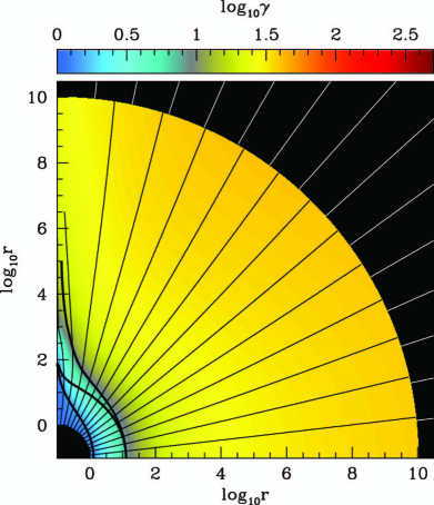
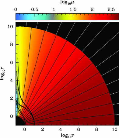
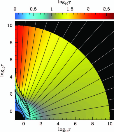
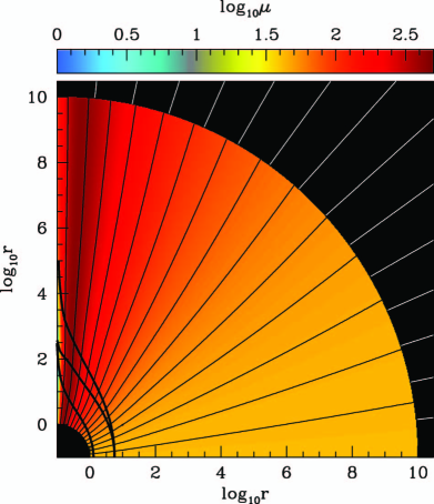
Figure 1.— Results for models M90 (upper panels) and M10 (lower panels). Radial dark lines show, for the steady state solution, the poloidal structure of field lines from $\log_{10}r=0$ (the surface of the star) to $\log_{10}r=10$. The white radial lines on the outside show the initial non-rotating monopolar configuration of field lines. The three thick solid lines correspond to the Alfvén surface (innermost), the fast surface (middle), and the causality surface (outermost, see §5.2). The fast surface and the causality surface touch each other at the midplane ($\theta=\pi/2$). Top-left: color-coded Lorentz factor $\gamma$ in model M90. Top-right: color-coded energy flux per unit mass flux $\mu$ in M90. Bottom-left: $\gamma$ in M10. Bottom-right: $\mu$ in M10. In the figure we use “logarithmic” spherical polar coordinates ($r_{l}=1+\log_{10}r\,,\theta_{l}=\theta$). The numbers along the horizontal (vertical) axis correspond to the values of $\log_{10}r$ along that axis, i.e., $r_{l}\cos\theta_{l}-1$ ($r_{l}\sin\theta_{l}-1$). Even though in these “logarithmic” polar coordinates the flow appears to over-collimate toward the axis (e.g., the two leftmost field lines on the upper panels), in fact $dR/dz$ remains positive everywhere in the solution. We note that the shape of the shown portion of the Alfvén surface is very close to a cylinder $R=1/\Omega=4/3$.

Consider first the shapes of the field lines in the poloidal plane. We see that, over most of the solution, the field lines are only slightly perturbed from their initial purely radial configuration. This might be surprising since rotation causes the toroidal component of the field to grow substantially. In fact, over most of the solution, $B_{\varphi}$ is tens of times larger than the poloidal field $B_{p}\equiv\sqrt{B_{r}^{2}+B_{\theta}^{2}}$, and one might think that the hoop stress of the strong toroidal field would cause substantial collimation of the field lines. This does not happen because the relativistic wind sets up an electric field, and an associated electric force per unit volume $\rho_{e}\vec{E}$ (charge density $\rho_{e}$), that almost exactly cancels the magnetic hoop stress. This is a unique feature of relativistic winds. It has been explored in detail by Narayan et al. (2007) and Tchekhovskoy et al. (2008, hereafter TMN08) in connection with winds in the force-free approximation (McKinney, 2006a; McKinney & Narayan, 2007b).

While it is true that the distortion of field lines in the poloidal plane is small, nevertheless, there is some distortion. It is especially obvious near the rotation axis, where we see field lines converging towards the pole and bunching up. In fact, very close to the rotation axis, the distortion appears to be quite large. Thus, the results indicate that the polar regions of a rotating monopole wind are qualitatively different from the equatorial regions of the outflow.

We next consider the acceleration of the wind. The top left panel of Fig. 1 shows the Lorentz factor $\gamma$ as a function of position. We see that there is an inner acceleration zone extending out to a radius $r\sim 10^{2}$, where the Lorentz factor increases from its initial small value ($\approx 1.2$ at the stellar surface). Beyond this we find a large coasting zone where there is very little change in $\gamma$. Over most of the coasting zone, the flow reaches ultrarelativistic Lorentz factors of $\gamma\sim 40$; however, this value is much less than expected if all the available free magnetic energy were to be used.

An axisymmetric magnetized wind has several conserved quantities along field lines. Two of these are the enclosed magnetic flux $\Phi$ and the angular velocity $\Omega$. Another is the ratio of poloidal magnetic flux to rest-mass flux (Chandrasekhar, 1956; Mestel, 1961; Li et al., 1992; Beskin, 1997):

$$\eta(\Phi)=\frac{\gamma\rho v_{p}}{B_{p}}={\rm const.}{\rm\ along\ field\ line.}$$ (4)

Yet another conserved quantity is the quantity $\mu$, which is the ratio of the total energy flux to the rest-mass flux (Chandrasekhar, 1956; Mestel, 1961; Lovelace et al., 1986; Begelman & Li, 1994; Beskin, 1997; Chiueh et al., 1998):

$$\mu(\Phi)=\frac{\mathcal{S}+\mathcal{K}}{\mathcal{R}}=\frac{E\left|B_{\varphi}\right|+\gamma^{2}\rho v_{p}}{\gamma\rho v_{p}}={\rm const.\ along\ field\ line}.$$ (5)

Here, ${\mathcal{S}}$ is the Poynting flux, ${\mathcal{K}}$ is the mass energy flux (rest mass $\mathcal{R}$ plus kinetic energy), $B_{\varphi}$ is the toroidal field,

$$E=\Omega RB_{p}$$ (6)

is the poloidal electric field, and $\rho$ is the mass density in the comoving frame of the fluid. The denominator of equation (5) is the rest mass flux. Since we consider highly magnetized winds, we have ${\mathcal{S}}\gg{\mathcal{K}}$ at the surface of the star. Moreover, at $r=1$ in the monopolar flow (Michel, 1969, 1973),

$$\left|B_{\varphi}\right|\approx E\approx\Omega\sin\theta_{\rm fp},$$ (7)

where $\theta_{\rm fp}$ represents the value of $\theta$ at the footpoint of a field line. Also, at the footpoint, $v_{p}$ and $\rho$ are constant, and $\gamma\approx 1$. We thus have

$$\mu(\theta_{\rm fp})\propto\sin^{2}\theta_{\rm fp},$$ (8)

for $\mu\gg\gamma_{0}$ ($\gamma_{0}$ is the initial Lorentz factor at $r=1$), i.e., $\mu$ is a rapidly increasing function of $\theta_{\rm fp}$. This can be seen in the top right panel in Fig. 1 and also in Fig. 2.

As mentioned above, the quantity $\mu$ is conserved along each field line. However, the two energy contributions to $\mu$, the Poynting flux ${\mathcal{S}}$ and the mass energy flux ${\mathcal{K}}$, are not individually conserved. In fact, the outflowing wind converts Poynting flux to mass energy, thereby accelerating the wind and causing $\gamma$ to increase.

If the wind were maximally efficient at accelerating the matter, we would expect ${\mathcal{S}}\to 0$ at large distance from the star. The Lorentz factor would then achieve its maximum value

$$\gamma_{\rm max}=\mu.$$ (9)

In practice, the wind falls far short of this maximum. As Figs. 1 and 2 show, $\mu$ is quite large in model M90, with a value of 460 at the equator ($\theta_{\rm fp}=\pi/2$). However, the Lorentz factor of the wind, even at a radius of $10^{10}$, does not exceed $40$. Thus, a magnetized monopole wind is very inefficient at accelerating the gas. For an equatorial field line in M90, the efficiency factor $\gamma/\mu$ is only about $0.09$, as shown in Fig. 2.

Another way of describing the efficiency of conversion of energy from electromagnetic to kinetic form is via the magnetization parameter $\sigma$, which is the ratio of Poynting to mass energy flux (Kennel & Coroniti, 1984a; Li et al., 1992; Begelman & Li, 1994; Vlahakis, 2004; Komissarov et al., 2007),

$$\sigma=\frac{\mathcal{S}}{\mathcal{K}}=\frac{E\left|B_{\varphi}\right|}{\gamma^{2}\rho v_{p}}.$$ (10)

Substituting into equation (5) we see that the conserved quantity $\mu$ is related to $\sigma$ by

$$\mu=\gamma(\sigma+1).$$ (11)

The smallest value possible for $\sigma$ is zero. Therefore, the maximum value of $\gamma$ is $\gamma_{\rm max}=\mu$ (eq. 9).

The magnetization $\sigma$ is not conserved along a field line. At the surface of the star, where $\gamma\approx 1$, we have $\sigma\approx\mu-1$. As the magnetized wind flows out and energy is transferred from Poynting to matter energy, $\gamma$ increases and $\sigma$ decreases. An efficient wind would be one in which $\sigma$ asymptotes to a value $\leq 1$, so that the outflowing material is able to convert at least half of its energy flux into matter energy. The numerical solutions shown in Figs. 1 and 2 fail to satisfy this criterion by a large factor in the equatorial regions. This implies there is no ideal, axisymmetric MHD solution to the $\sigma$-problem (Rees & Gunn, 1974; Kennel & Coroniti, 1984a; Kennel & Coroniti, 1984b).

There is, however, one promising feature in the results: the polar regions of the wind are efficient, with $\gamma/\mu\to 1$ and $\sigma\ll 1$ at large distance from the star (Fig. 2). This interesting feature of the monopole problem has not been emphasized in the literature. Most previous analyses and discussions have focused on equatorial field lines where the efficiency is, indeed, too low to solve the $\sigma$ problem.

Unfortunately, the actual Lorentz factor along polar field lines in M90 is only $\sim 20$ since this is the value of $\mu$ for these lines. Would we continue to have high efficiency in the polar region even with larger values of $\mu$? In particular, is it possible to have acceleration with high efficiency up to Lorentz factors $\gamma>100$, as observed for instance in gamma-ray bursts? For this we need to study a model with larger values of $\mu$ near the pole. We describe such a model in the next subsection.

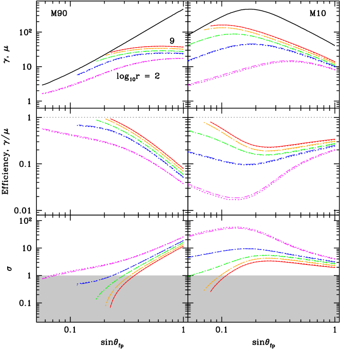
Figure 2.— The panels on the left correspond to model M90 and those on the right to M10. The solid black lines in the top panels show the scaled total energy flux $\mu$ as a function of $\sin\theta_{\rm fp}$, where $\theta_{\rm fp}$ is the polar angle corresponding to footpoints of field lines. The five colored lines show profiles of $\gamma$ at five different distances from the star: $r=10^{2}$ (magenta, dash–dotted), $10^{3}$ (blue, long-short–dashed), $10^{4}$ (green, short–dashed), $10^{6}$ (orange, long–dashed), $10^{9}$ (red, solid). The closer $\gamma$ gets to $\mu$ the more efficient the acceleration. The middle panels show the acceleration efficiency $\gamma/\mu$ and the lower panels show the magnetization parameter $\sigma=(\mu/\gamma)-1$ at the same five distances. Note that $\gamma/\mu$ is largest and $\sigma$ is smallest closest to the pole ($\sin\theta_{\rm fp}\ll 1$). The various dotted lines correspond to the analytical model described in §4.1. The shaded area in the bottom panel indicates the regions of the solution where mass energy flux exceeds Poynting flux ($\sigma<1$, or $\gamma/\mu>1/2$). Note that magnetic flux gradually converges toward the polar axis as a function of increasing radius, so the lines corresponding to larger radii truncate at small values of $\theta_{\rm fp}$.

3.2. Model M10

From equation (5) we see that an obvious way to increase $\mu$ is to lower the density of the wind at the stellar surface. For instance, if we were to reduce $\rho$ by a factor of $\sim 30$ relative to M90, then we would have a model with $\mu\sim$  few hundred for a field line with $\theta_{\rm fp}\sim 10^{\circ}$ (see Fig. 3). We could then explore acceleration along this field line and determine whether or not the outflowing wind achieves a coasting $\gamma>100$.

Since $\mu$ varies as $\sin^{2}\theta_{\rm fp}$, this approach would lead to extremely large values of $\mu$ at the equator. As a result, the model would require very large resolution to simulate accurately and would be extremely expensive. Therefore, for numerical convenience, we consider a model in which we choose the profile $\rho(\theta_{\rm fp})$ such that $\mu$ is large near the pole, reaches a maximum $\mu_{\rm max}$ at a specified footpoint angle $\theta_{\rm fp}=\theta_{\rm max}$, and then decreases with increasing $\theta_{\rm fp}$ to an outer value $\mu_{\rm out}$ at $\theta_{\rm fp}=\pi/2$. To achieve this, we choose the density profile on the star to be

$$\rho(\theta_{\rm fp})=\rho_{0}+\rho_{1}\sin^{\alpha}\theta_{\rm fp},$$ (12)

where the constants $\rho_{0}$, $\rho_{1}$ and $\alpha$ are adjusted so that the model has the desired values of $\mu_{\rm max}$, $\theta_{\rm max}$ and $\mu_{\rm out}$.

We have simulated a series of such models, all with $\mu_{\rm max}=460$ and $\mu_{\rm out}=40$ , and with different values of $\theta_{\rm max}$, viz., $45^{\circ}$, $20^{\circ}$, $10^{\circ}$, which we refer to as models M45, M20, M10, respectively. Figure 3 shows the profiles of $\rho(\theta_{\rm fp})$ and $\mu(\theta_{\rm fp})$ for the model M10. Parameters of the various models are summarized in Table 1. The models are well-converged, with field-line invariants $\Omega(\Phi)$, $\eta(\Phi)$, and $\mu(\Phi)$ conserved along field lines to better than $15$%, as Fig. 4 shows for, e.g., models M90 and M10.

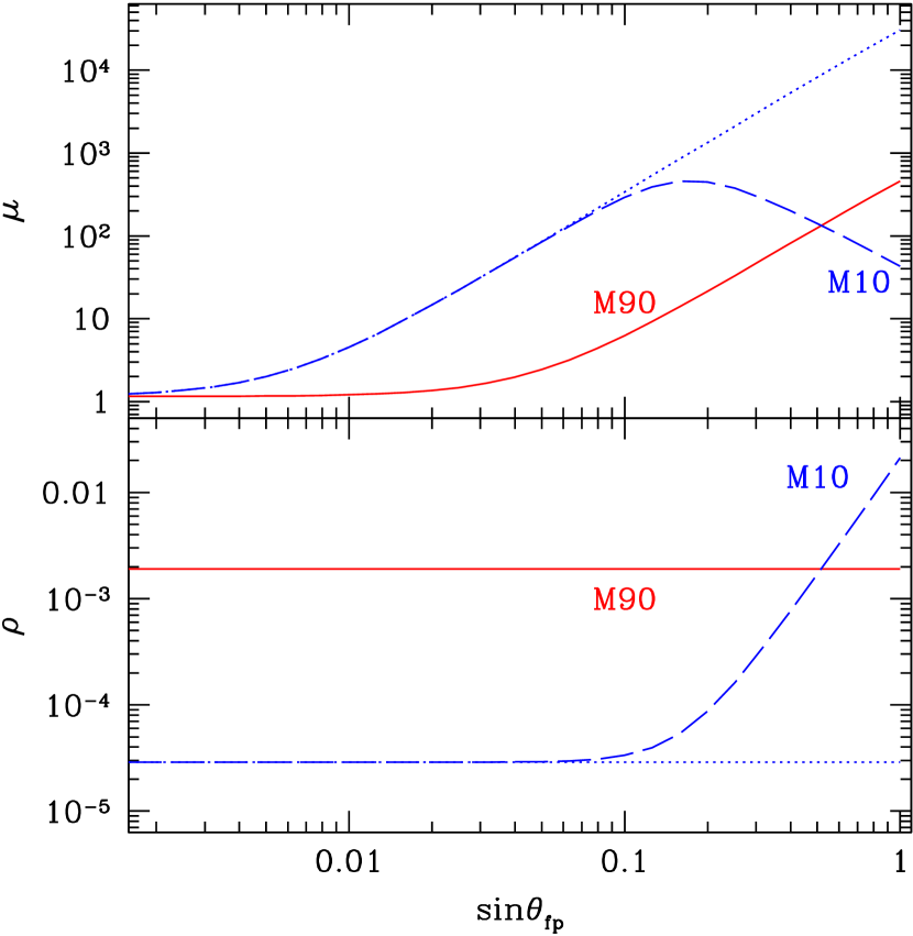
Figure 3.— The red lines in the two panels show the distribution of $\mu$ and $\rho$ as a function of footpoint angle $\theta_{\rm fp}$ in the baseline model M90. The blue dotted lines show the corresponding profiles for a hypothetical model in which $\rho$ is decreased by a constant factor, leading to an increase in $\mu$ by the same factor. Since this causes $\mu$ to become very large at the equator, leading to numerical difficulties, we consider the model M10 (dashed blue lines) that has the same behavior of $\mu$ and $\rho$ near the axis but is less extreme near the equator. In both models M10 and M90 the matter-dominated part of the flow $\mu\sim 1$ at the surface of the star is resolved on the grid by at least several grid cells.

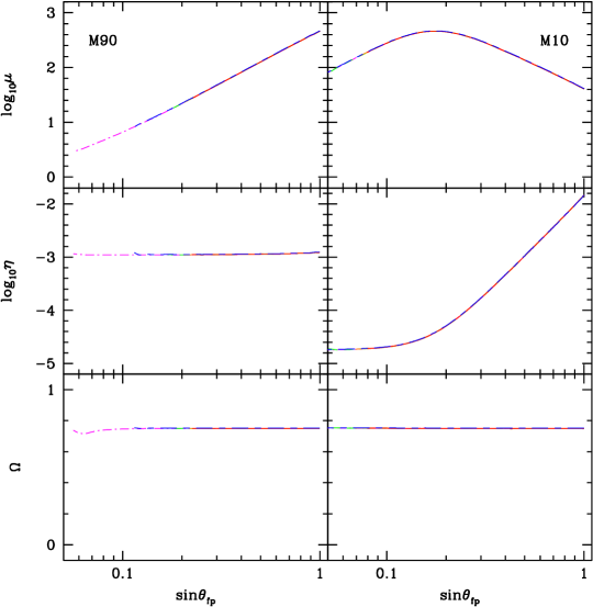
Figure 4.— The panels on the left correspond to model M90 and those on the right to M10. The five colored lines correspond to $r=10^{2}$, $10^{3}$, $10^{4}$, $10^{6}$, and $10^{9}$ (see Fig. 2 for a description of line colors and types) and show profiles of quantities that are preserved along the field lines: $\mu(\theta_{\rm fp})$ (the top panel), $\eta(\theta_{\rm fp})$ (the middle panel), and $\Omega(\theta_{\rm fp})$ (the bottom panel). These lines nearly overlap each other, as expected for a flow in steady state. In the numerical simulations, each of the quantities is preserved along field lines to better than $15$%. A few grid cells from the polar axis, within which unresolved magnetic flux accumulates, are least accurate (not shown); but as we have checked, this does not affect the quality of the solution at larger angles (see end of §4.4).

The bottom two panels in Fig. 1 show results corresponding to M10. As before, we see that the poloidal structure of the field is largely unaffected by rotation. There is of course some lateral shift of field lines, the effect being larger near the pole than near the equator, with maximum field line bunching close to the axis.

The Lorentz factor distribution again confirms the trends seen in M90. Near the equator, the asymptotic $\gamma$ is only $\sim 12$, giving an inefficient flow with $\gamma/\mu\sim 0.3$. The efficiency increases near the axis and becomes practically equal to unity close to the pole; equivalently, $\sigma$ becomes much less than unity for these field lines. Most interestingly, Lorentz factors nearly as large as $\sim 200$ are obtained for these field lines. In other words, there is no $\sigma$ problem near the axis and it is possible to obtain quite large Lorentz factors in this region of the outflow.

3.3. Summary of Key Results

From the results shown in Figs. 1, 2, we conclude the following:

1. Field lines near the equator of a rotating monopole largely retain their monopolar configuration out to large radii, whereas lines near the pole tend to bunch up around the axis.

2. The acceleration efficiency $\gamma/\mu$ of a rotating monopole magnetosphere is low ($\ll 1$) for field lines in the equatorial region, but quite high ($\sim 1$) for field lines near the pole.

We would like to develop an understanding of the physics behind of these effects. We would also like to know how the two effects are related to each other. This is the topic of the next two sections.

4. Field Line Bunching

4.1. Relation to Acceleration Efficiency

As plasma streams along field lines, relativistic effects become important near the so-called light cylinder, $R=R_{\rm L}=1/\Omega$, where the co-rotation velocity $\Omega R$ equals the speed of light and $E=B_{p}$ (see eq. 6). As we show in Appendix A, far outside the light cylinder, where $\Omega R\gg 1$ and $\gamma\gg\gamma_{0}$, the plasma simply drifts perpendicular to $\vec{E}$ and $\vec{B}$ at the drift velocity (Beskin et al., 1998, 2004; Vlahakis, 2004),

$$v\approx v_{\rm dr}=\left|\frac{\vec{E}\times\vec{B}}{B^{2}}\right|=\frac{E}{B},$$ (13)

The corresponding Lorentz factor is

$$\gamma^{2}\approx\gamma_{\rm dr}^{2}=\frac{B^{2}}{B^{2}-E^{2}}.$$ (14)

Near the star this formula becomes inaccurate since the plasma moves at the initial Lorentz factor,

$$\gamma^{2}\approx\gamma_{0}^{2}.$$ (15)

In Appendix A we show that a combination of these two formulae does a very good job of describing the Lorentz factor at all distances from the star:

$$\gamma^{2}=\gamma_{0}^{2}-1+\gamma_{\rm dr}^{2}.$$ (16)

In the asymptotic region of a relativistic outflow (where $\Omega R\gg 1$, $\gamma\gg 1$), we have according to (14),

$$\left|B_{\varphi}\right|\approx E.$$ (17)

Further, this relation is also true at the surface of the central compact star (for the monopolar flow, see eq. 7). This allows us to write the difference between the maximum allowed Lorentz factor $\gamma_{\rm max}=\mu$ and the local Lorentz factor $\gamma$ in the following convenient form (the numbers in parentheses refer to the equations used to derive this result):

$$\mu-\gamma\overset{\eqref{eq_mudef},\eqref{eq_EBsurface},\eqref{eq_eb_asymptotic}}{\approx}\frac{E^{2}}{\gamma\rho v_{p}}\overset{\eqref{eq_etadef}}{=}\frac{(\Omega RB_{p})^{2}}{\eta B_{p}}=\frac{\Omega^{2}(\Phi)}{\eta(\Phi)}{B_{p}R^{2}}.$$ (18)

By dividing this equation by itself as evaluated at the footpoint, and approximating $\gamma-\gamma_{\rm fp}\approx\gamma$ and $\mu-\gamma_{\rm fp}\approx\mu$, we obtain

$$\frac{\gamma}{\mu}\approx 1-\frac{B_{p}R^{2}}{[B_{p}R^{2}]_{\rm fp}}\approx 1-\frac{a}{a_{\rm fp}},$$ (19)

where we have used the subscript “fp” to denote quantities evaluated at the field line footpoint and have defined the quantity

$$a\equiv B_{p}R^{2}.$$ (20)

Equation (19) demonstrates that, in order to convert an appreciable fraction of the total energy flux $\mu$ along a field line into matter energy flux ($\gamma$ times the mass flux), the quantity $a$ has to decrease appreciably from its initial value at the footpoint. This result is known (c.f. Begelman & Li, 1994; Chiueh et al., 1998; Vlahakis, 2004), though we have not seen as simple a derivation as the one given above.

For a precisely monopole field, $B_{p}\propto 1/R^{2}$ along each field line. Therefore, $a=B_{p}R^{2}$ is constant along a field line and so no efficient acceleration is possible. This explains why acceleration is so difficult in the monopole problem. In order to permit acceleration, field lines must move in a cooperative fashion transverse to one another so as to allow $a$ to reduce with increasing distance from the star. We discuss how this is accomplished in the next subsection.

Meanwhile, as an aside, we describe here an improvement to the approximate result  (19) which gives the correct numerical value of efficiency in a precisely monopolar field. For such a field, the Lorentz factor at asymptotically large distances is (Michel, 1969; Camenzind, 1986)

$$\gamma_{\infty}^{\mathrm{radial}}=\mu^{1/3}\ll\mu.$$ (21)

This gives an extremely inefficient acceleration, $\gamma/\mu\approx\mu^{-2/3}\ll 1$. However, the efficiency is not zero as equation (19) might suggest, so we need a more accurate version of (17). According to (14),

$$B_{\varphi}\approx\frac{\gamma E}{\sqrt{\gamma^{2}-1}}=\frac{\gamma\Omega RB_{p}}{\sqrt{\gamma^{2}-1}}\approx\Omega RB_{p}\left(1+\frac{1}{2\gamma^{2}}\right).$$ (22)

Using this equation, assuming $B_{p}R^{2}={\rm const.}$ along a field line, and introducing $\gamma_{\infty}=\lim_{R\to\infty}\gamma$, we obtain in the limit $R\to\infty$

$$\mu(\Phi)\approx\gamma_{\infty}+\frac{\Omega^{2}(\Phi)}{\eta(\Phi)}B_{p}R^{2}\left(1+\frac{1}{2\gamma_{\infty}^{2}}\right).$$ (23)

Now, assuming that the system settles down to a state with minimum total energy flux $\mu(\Phi)$ (equivalent to the minimal torque condition of Michel 1969), we find the terminal Lorentz factor $\gamma_{\infty}$ that minimizes the right hand side of this equation:

$$\gamma_{\infty}^{\mathrm{radial}}=\left[\frac{\Omega^{2}(\Phi)}{\eta(\Phi)}B_{p}R^{2}\right]^{1/3}\approx\mu^{1/3},$$ (24)

where the approximate equality comes from equation (18) evaluated at the footpoint. This reproduces (21) and shows that indeed, for a precisely radial flow, only a small (but still non-zero) fraction of the Poynting flux is converted to the kinetic energy of the matter. This derivation was performed for precisely monopolar field lines. In actuality the shape of the poloidal field lines is slightly changed from radial. The effect is small for equatorial field lines and the order of magnitude estimate (24) continues to hold. The deviations are larger for polar field lines and the Lorentz factor obtained along these lines is very different from (24).

4.2. Field Lines Near the Midplane

Let us first apply formula (19) to a field line near the midplane. For acceleration to be efficient, $a$ must decrease along the field line, i.e., $B_{p}$ must decrease faster than $1/R^{2}$. This can be accomplished by moving field lines away from the equator towards the axis. Consider a field line with its footpoint located at a small angle $\theta^{\prime}_{\rm fp}=\pi/2-\theta_{\rm fp}\ll 1$ from the equator. For this field line we can write (19) as

$$\frac{\gamma}{\mu}\approx 1-\frac{a}{a_{\rm fp}}\approx 1-\frac{\theta^{\prime}_{\rm fp}}{\theta^{\prime}},$$ (25)

where $\theta^{\prime}$ is the polar angle of the field line at a large distance from the star, where the Lorentz factor is $\gamma$. Here we used the fact that $\Phi^{\prime}\approx 2\pi a\,\theta^{\prime}\approx 2\pi a_{\rm fp}\theta^{\prime}_{\rm fp}$, where $\Phi^{\prime}$ is the amount of flux enclosed between the field line and the midplane.

For a nearly monopolar configuration of the field in which $\theta^{\prime}\approx\theta^{\prime}_{\rm fp}$, obviously we will not have much acceleration ($\gamma/\mu\ll 1$). In order to obtain high acceleration efficiency in the equatorial region, field lines must diverge from the equator so that the $\theta^{\prime}$ values of field lines increase with distance. For this to happen, the rest of the magnetosphere must collectively move away from the equator towards the pole. For reasons that are discussed in §5, this does not happen, and so acceleration efficiency is at best modest near the equator.

4.3. Polar Field Lines

The story is quite different for field lines close to the axis ($\theta\ll 1$). Consider the initial undistorted monopole configuration. At the surface of the star, $B_{p}$ is constant, and $[B_{p}R^{2}]_{\rm fp}$ is simply equal to $\Phi/\pi$, where $\Phi$ is the flux interior to the field line. For a pure monopole, this relation is valid at any distance from the star, i.e., $B_{p}R^{2}=\Phi/\pi$ at all radii, and therefore $a/a_{\rm fp}=1$ and acceleration would be inefficient.

In analogy with the previous discussion for equatorial field lines, let us now imagine uniformly expanding or contracting the field lines near the axis. That is, for each field line with a given $\theta_{\rm fp}\ll 1$, let the polar angle far from the star become $\theta=k\theta_{\rm fp}$, with the same value of $k$ for all lines. For such a uniform expansion or contraction of the field, $B_{p}$ transforms to $B_{p}/k^{2}$. However, at the same time $R$ becomes $kR$, and so $a=B_{p}R^{2}$ is unaffected. In other words, there is no effect on acceleration.

The key to obtaining acceleration along polar field lines is not uniform lateral expansion (divergence) or contraction (collimation) of field lines, but differential bunching of field lines. To see this rewrite equation (19) as

$$\frac{\gamma}{\mu}\approx 1-\frac{a}{a_{\rm fp}}\approx 1-\frac{\pi B_{p}R^{2}}{\Phi},$$ (26)

where we have used the fact that $a_{\rm fp}\approx\Phi/\pi$ near the pole. Clearly, for efficient acceleration, we must make $B_{p}$ substantially smaller than the mean enclosed field $\Phi/\pi R^{2}$. That is, the field lines interior to the reference field line must be bunched in such a way that most of the flux has been pulled inward. As an example, consider a power-law distribution of the field strength,

$$B_{p}(R)\propto R^{-\xi},$$ (27)

where the index $\xi$ measures the degree of bunching. This distribution gives

$$\frac{\gamma}{\mu}\approx\frac{\xi}{2},$$ (28)

which shows that the acceleration efficiency increases with increasing $\xi$. We reach equipartition between Poynting and matter energy flux ($\sigma\sim 1$, $\gamma\sim\mu/2$) for $\xi=1$, and we obtain arbitrarily large efficiency ($\sigma\ll 1$) as $\xi\to 2$.

As we have described in §3, polar field lines in simulation M90 are very efficient with $\gamma/\mu\to 1$. According to the above, this would seem to suggest that $\xi(R)$ should be $\approx 2$ at the axis and should decrease with increasing $R$. The simulations, however, show that this does not happen: as we show later, $\xi\approx 1$, i.e., it stays roughly constant over a range of $R$. Instead, higher efficiency near the jet axis is achieved in a different way: as field lines bunch around the jet axis (Chiueh et al., 1991; Eichler, 1993; Bogovalov, 1995; Bogovalov & Tsinganos, 1999), they form a concentrated core (Heyvaerts & Norman, 1989; Bogovalov, 2001; Lyubarsky & Eichler, 2001; Beskin & Nokhrina, 2008) that takes up a finite amount of flux $\Phi_{0}$, leading roughly to the following poloidal field strength profile

$$B_{p}(R)=\Phi_{0}\delta(\pi R^{2})+B_{0}(R/R_{0})^{-\xi},$$ (29)

where we have approximated the core profile with the Dirac delta-function. This gives

$$\frac{\gamma}{\mu}\approx\begin{cases}{\xi}/{2},\quad&\Phi_{0}\ll\pi B_{p}R^{2}/(1-\xi/2),\\ 1-{\pi B_{p}R^{2}}/{\Phi_{0}},\quad&\Phi_{0}\gg\pi B_{p}R^{2}/(1-\xi/2).\end{cases}$$ (30)

That is, in the limit when the flux in the concentrated core is small compared to the flux in the surrounding power-law field distribution, the efficiency is the same as in (28). However, in the opposite limit, i.e., sufficiently close to the core where the flux in the core dominates, the angular profile of the poloidal field distribution (and the value of $\xi$) become irrelevant for determining the acceleration efficiency. Thus, (1) differential bunching and (2) the resulting development of a concentrated core, are the key requirements for efficient acceleration.

Note the following important corollary from the above discussion. It does not matter whether the particular field line of interest collimates towards the axis or diverges from it. This has no effect on the acceleration. What we need is that (1) other field lines closer to the axis must converge more, or diverge less, compared to the reference field line, and/or (2) a concentrated core at the jet axis must contain a significant amount of magnetic flux.

4.4. Comparison with Numerical Results

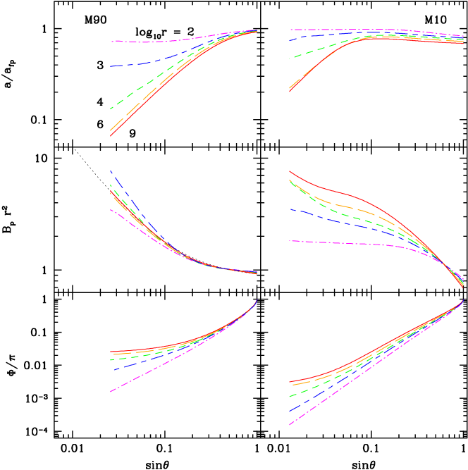
Figure 5.— The panels on the left correspond to model M90 and those on the right to M10. The five curves correspond to different distances from the star: $r=10^{2}$, $10^{3}$, $10^{4}$, $10^{6}$, $10^{9}$ (see Fig. 2 for a description of line colors and types). The top panels show the quantity $a/a_{\rm fp}$, which determines the acceleration along a field line. Note that $a/a_{\rm fp}$ is smallest near the poles, where Fig. 2 shows the largest acceleration. The middle panels show the profiles of normalized field strength $B_{p}r^{2}$ at the same five distances. Notice the nonuniform distribution as a function of angle. This is necessary for acceleration, as explained in §4.3. In the middle-left panel the curved dotted line corresponds to (31) and accurately describes the angular profile of $B_{p}$ at large distances. The lower panels show the angular distribution of the flux function $\Phi/\pi$.

Figure 5 shows results for models M90 and M10. The top panels show the behavior of $a/a_{\rm fp}$ at different distances from the central star. We see that $a/a_{\rm fp}$ decreases towards the pole, exactly where $\gamma/\mu$ is largest and $\sigma$ is smallest in Fig. 2. Also, Fig. 2 quantitatively confirms the validity of equation (19) by plotting prediction (19) over the numerical solution.

The lower panels in Fig. 5 illustrate the effects described in the previous two subsections. In the equatorial regions, we see that $B_{p}r^{2}$ decreases from its footpoint value of unity. It is this decrease that allows whatever acceleration is observed in this region of the outflow. However, the decrease is modest, so the acceleration is not very large.

For angles closer to the pole, $B_{p}r^{2}$ actually increases relative to its nominal initial value of unity. Nevertheless, this does not mean that there is deceleration because, as we argued above, acceleration near the axis is associated with differential bunching, not with any overall expansion or contraction. For both M90 and M10, we see that the magnetic field sets up the required bunching so that the poloidal field is maximum at the axis and decreases with increasing distance from the pole. It is this outward decrease, coupled with the presence of magnetic flux $\Phi_{0}$ in a concentrated core at the pole (see eq. 30), that is associated with a decrease in $a/a_{\rm fp}$ for polar field lines and the reason for strong acceleration.

The effect is most clearly seen in model M90, as illustrated in Fig. 5. Between $r=10^{2}$ and $r=10^{3}$ the angular profile of $B_{p}$ becomes a steeper function of polar angle, leading to an associated decrease in $a/a_{\rm fp}$. Between $r=10^{3}$ and $r=10^{4}$ the trend reverses, and the poloidal field profile actually becomes a shallower function of polar angle; however, $a/a_{\rm fp}$ continues to decrease. Beyond $r\sim 10^{4}$ the magnetic field profile does not evolve further. In this regime it can be well-fitted by a broken power-law,

$$B_{p}r^{2}=0.85+0.075\sin^{-1.1}\theta.$$ (31)

Therefore at these distances $a=B_{p}r^{2}\sin^{2}\theta$ does not evolve with $r$ either. Despite this, $a/a_{\rm fp}\approx\pi a/\Phi$ decreases with increasing $r$ and the value of $\Phi$ increases. This is solely due to the increase in the amount of magnetic flux $\Phi_{0}$ contained in the concentrated core.

The picture that emerges is the following. The poloidal magnetic field establishes some equilibrium angular profile $B_{p}(r,\theta)r^{2}$ at intermediate latitudes that does not evolve with $r$. At progressively larger $r$, each individual magnetic field line becomes progressively more collimated towards the pole, but the same angular profile of magnetic field is maintained. This means that magnetic flux $\Phi$ flows out from the low-latitude equatorial region ($B_{p}$ slightly decreases there), flows through intermediate latitudes without changing the profile of $B_{p}$ there, and ends up in the concentrated core at the polar axis, thereby uniformly shifting the angular poloidal flux distribution $\Phi(\theta)$ up. The effect is clearly seen in the lower-left panel of Fig. 5.

Note that it is not necessary to numerically resolve the concentrated core in order to accurately describe the jet structure since it is only the total amount of magnetic flux contained in the concentrated core that matters for the acceleration efficiency. In particular, our numerical method is well-suited for capturing such a core, even if unresolved, since our method conserves the magnetic flux to machine precision and can accurately capture the amount of magnetic flux that enters the core and remains there. We note that within a few grid cells from the polar axis, where the unresolved magnetic flux accumulates, are least accurate but this does not affect the quality of the solution at larger angles. To verify this, we have checked convergence of our models with angular resolution. For this, we ran a version of model M90 that uses a uniform angular grid and has a factor of $2$ lower effective angular resolution near the pole. Using this less-resolved model leads to a maximum relative difference in the flux function $\Phi$ and Lorentz factor of less than $15$%, even near the rotation axis. This difference is less than $2$% at most radii ($r<10^{2}$ and $r>10^{5}$) and is smaller at larger $\theta$. This confirms the accuracy of the numerical solution. Future higher-resolution models that resolve smaller angles and the concentrated core are required to determine how the solution connects the polar axis and for independent verification of results.

5. Acceleration Efficiency and Communication with the Axis

5.1. Fast Magnetosonic Surface

Beskin et al. (1998) have discussed the physical reason for inefficient acceleration in the equatorial regions. They show that it is related to the fast magnetosonic point. In the comoving frame of a cold MHD plasma, fast magnetosonic waves travel with a speed $v_{f}$ given by (Gammie et al., 2003; McKinney, 2006b)

$$\gamma_{f}v_{f}=\left(\frac{b^{2}}{\rho}\right)^{1/2},$$ (32)

where $b$ is the comoving magnetic field strength. It is straightforward to relate $b$ to field components in the lab frame:

$$b^{2}=B^{2}-E^{2}\overset{\eqref{eq_gammadrift}}{\approx}\frac{B^{2}}{\gamma^{2}}\overset{\eqref{eq_eb_asymptotic}}{\approx}\frac{E\left|B_{\varphi}\right|}{\gamma^{2}}\overset{\eqref{eq_sigmadef}}{\approx}\rho\sigma.$$ (33)

We thus find

$$\gamma_{f}v_{f}\approx\sigma^{1/2}.$$ (34)

Consider a streamline in the wind that moves outward with a local Lorentz factor $\gamma$. Let us first consider the limit of infinitely high magnetization, $\rho\to 0$, i.e. the force-free limit (Goldreich & Julian 1969; Okamoto 1974; Blandford 1976; Lovelace 1976; Blandford & Znajek 1977; MacDonald & Thorne 1982; Fendt et al. 1995; Komissarov 2001, 2002a, 2002b; McKinney 2006a; Narayan et al. 2007; TMN08). In this limit $\gamma_{f}\to\infty$, therefore throughout the solution we have $\gamma<\gamma_{f}$. This means that the fast magnetosonic surface, defined by the condition $\gamma=\gamma_{f}$, where the wind becomes causally detached from fluid farther back along its streamline, is located at infinity. Such a force-free wind has a simple analytic solution in which the Lorentz factor increases roughly linearly with distance (Michel, 1973),

$$\gamma\approx\Omega R.$$ (35)

In general, $\rho\neq 0$, yet we might expect that the behavior of the Lorentz factor in the sub-fast region $\gamma<\gamma_{f}$ is similar to the force-free solution (35). This has been shown to indeed be the case (Beskin et al., 1998). However, the acceleration in the super-fast region $\gamma>\gamma_{f}$ has been found to become logarithmic, i.e. inefficient (Beskin et al., 1998). Once the wind has crossed the fast magnetosonic point $\gamma=\gamma_{f}$, it becomes causally detached from the fluid farther back along its streamline. We might therefore expect efficient acceleration to cease beyond this fast magnetosonic point for all field lines.

If we define the fast Mach number $M_{f}$ by

$$M_{f}=\frac{\gamma v}{\gamma_{f}v_{f}}\approx\frac{\gamma v}{\sigma^{1/2}},$$ (36)

then the fast point is the location at which $M_{f}\approx 1$ (this equality would be exact if there was only motion along the poloidal field line; however, there is also a slow rotation in the toroidal direction which introduces a negligible correction that we ignore). For a relativistic flow ($v\approx 1$), equation (11) lets us recast the above expression in a useful form:

$$M_{f}^{2}\approx\frac{\gamma^{2}}{\sigma}=\frac{\gamma^{3}}{\mu-\gamma}.$$ (37)

Figure 6 shows results for a field line in M90 with $\theta_{\rm fp}=\theta=\pi/2$. Until the flow reaches the fast magnetosonic point, we see that $\sigma$ falls rapidly and $\gamma$ increases rapidly. However, both trends slow down substantially once the flow crosses the fast point. Beyond this point, Beskin et al. (1998) have shown that $\sigma$ and $\gamma$ vary as the one-third power of $\log r$. We confirm this dependence below.

Figure 6.— Dependence of various quantities as a function of distance for a field line with $\theta_{\rm fp}=\pi/2$ in model M90. [Top panel] Solid lines show the radial dependence of $\gamma$, $\sigma$, and $\mu$ from the simulation. [Bottom panel] The solid line shows the inverse of the fast Mach number $1/M_{f}$. The fast surface, indicated with the vertical dotted line, is located where $M_{f}=1$. This is also the location of the causality surface (41) for this field line. The various other dotted lines show the analytical approximation (49).

The relatively abrupt cessation of acceleration beyond the fast point for equatorial field lines is obvious in Fig. 1, where we see that $\gamma$ stops increasing once the flow crosses the fast magnetosonic surface (the middle of the three thick solid lines). However, it is also clear from Fig. 1 that something else operates on polar field lines. Model M10, in particular, shows substantial continued acceleration well after polar field lines have crossed the fast surface. We discuss next the relevant physics for these field lines.

5.2. Communication with the Axis: Causality Surface

We showed in §4 that, for efficient acceleration along a field line, other neighboring field lines must shift laterally. At the equator, we need lines to move away from the midplane, while near the pole, we need field lines to experience differential bunching or develop a flux core. In order for any given field line to sustain efficient energy conversion, it must be able to communicate to other regions of the magnetized wind that undergo differential bunching or cause a concentrated flux core. This suggests that the fast magnetosonic point, which determines where the fluid can no longer communicate back along its motion, is perhaps not so important. A more relevant issue is whether or not the fluid can communicate with regions near the axis that have field bunching or a flux core. We refer to the point at which a fluid element loses contact with the axis as the “causal point,” and call the locus of causal points over all field lines as the “causality surface”. By the above arguments, we expect that this surface, rather than the fast magnetosonic surface, plays the role of the boundary for efficient acceleration. We expect efficient acceleration inside this surface and inefficient, logarithmic acceleration outside the surface (for a related discussion, see Zakamska et al., 2008; Komissarov et al., 2009). In general fast waves propagate away from any given point toward the rotation axis through an intermediate region where the density, velocity, and magnetic field vary. Hence, one should trace the position of fast waves emitted from any given point outward over all angles and identify the “causal point” for each field line as where finally no such traces can reach the polar axis. For simplicity, we instead use only the local fast wave speed at a given point, and we identify the approximate “causal point” by where the locally emitted fast waves move away from any given point with a lab-frame local angle of $\theta>0$ with respect to the rotation axis, so that the waves do not reach the rotation axis over a finite propagation distance. We now calculate the approximate location of the causality surface using this approach.

Consider a segment of the relativistic magnetized wind propagating with a velocity vector $\vec{v}$ and Lorentz factor $\gamma$ at an angle $\theta_{j}$ to the rotation axis. In Appendix D we show that fast magnetosonic waves, which are emitted isotropically in the comoving frame of the fluid, in the lab frame will be collimated along $\vec{v}$ into a Mach cone with a half-opening angle

$$\sin\xi_{\rm max}=\frac{\gamma_{f}v_{f}}{\gamma v}=\frac{1}{M_{f}}.$$ (38)

By the argument given earlier, field line bunching and efficient acceleration are possible only when the fluid can communicate with the axis, i.e., only if $\xi_{\rm max}\gtrsim\theta_{j}$, i.e., only if

$$\sin\theta_{j}\lesssim\frac{1}{M_{f}}.$$ (39)

For an equatorial wind, i.e., $\theta_{j}=\pi/2$, equation (39) shows that acceleration stops when $M_{f}=1$, i.e., $\gamma=\gamma_{f}\approx\sigma^{1/2}$ (c.f. eq. 34, assuming $v_{f}\to 1$). That is, the wind stops efficient acceleration as soon as it crosses the fast magnetosonic point. However, for smaller values of $\theta_{j}$, we obtain a different result.

According to equation (38), communication with the axis and efficient acceleration are possible until

$$\gamma v\approx\frac{\gamma_{f}v_{f}}{\sin\theta_{j}}=\frac{\sigma^{1/2}}{\sin\theta_{j}}.$$ (40)

The presence of the factor $\sin\theta_{j}$ in the denominator means that communication extends to larger values of $\gamma$, i.e., acceleration efficiency becomes larger as $\theta_{j}$ decreases. In other words, polar field lines can accelerate more easily. Using the definition of the fast magnetosonic Mach number (36), we obtain the following relation for the causality surface:

$$\sin^{2}\theta_{j,c}\overset{\eqref{eq_gammabeta}}{=}\frac{1}{M_{f,c}^{2}}\overset{\eqref{eq_Mfsq}}{\approx}\frac{\sigma_{c}}{\gamma_{c}^{2}}=\frac{\mu-\gamma_{c}}{\gamma_{c}^{3}},$$ (41)

where the subscript “c” indicates quantities evaluated at the causality surface. Inside the causality surface we expect the Lorentz factor to increase roughly linearly with distance, c.f. eq. (35). Based upon our earlier arguments, once outside the causality surface the acceleration will only be logarithmic. Using (41), we can estimate the distance at which the causality surface is located:

$$r_{c}\sim\frac{\mu^{1/3}}{\Omega\sin^{5/3}\theta_{j,c}},$$ (42)

where we have assumed that (35) and $\gamma\ll\mu$ hold for $r\lesssim r_{c}$.

Figure 7.— Dependence of various quantities as a function of distance for a field line with $\sin\theta_{\rm fp}=0.1$ in model M10. [Top panel] Solid lines show the radial dependence of $\gamma$, $\sigma$, and $\mu$. [Bottom panel] The solid line shows the inverse of the fast Mach number $1/M_{f}$ and the dashed line shows the local opening angle of the field line $\theta_{j}$. The two vertical dotted lines indicate the positions of the fast magnetosonic point F ($M_{f}=1$) and the causality point C ($\sin\theta_{j}=1/M_{f}$). The various other dotted lines correspond to the analytical approximation (49).

Figure 8.— Dependence of various quantities as a function of distance for a field line with $\sin\theta_{\rm fp}=0.1$ in model W10. Comparison to Fig. 7 shows that the wall inhibits the collimation of field lines. This brings the causality surface closer to the central star than in the model without a wall, and hence leads to a lower efficiency here compared to M10. [Top panel] Solid lines show the radial dependence of $\gamma$, $\sigma$, and $\mu$. [Bottom panel] The solid line shows the inverse of the fast Mach number $1/M_{f}$ and the dashed line shows the local opening angle of the field line $\theta_{j}$. The two vertical dotted lines indicate the positions of the fast magnetosonic point F ($M_{f}=1$) and the causality point C ($\sin\theta_{j}=1/M_{f}$). The various other dotted lines correspond to the analytical approximation (49).

Figure 9.— Dependence of various quantities as a function of distance for a field line with $\sin\theta_{\rm fp}=0.06$ in model W5. [Top panel] Solid lines show the radial dependence of $\gamma$, $\sigma$, and $\mu$. [Bottom panel] The solid line shows the inverse of the fast Mach number $1/M_{f}$ and the dashed line shows the local opening angle of the field line $\theta_{j}$. The two vertical dotted lines indicate the positions of the fast magnetosonic point F ($M_{f}=1$) and the causality point C ($\sin\theta_{j}=1/M_{f}$). The various other dotted lines correspond to the analytical approximation (49).

Figure 1 confirms that the causality surface (the outermost of the three thick solid lines) provides a better approximation to the boundary between the acceleration and coasting zones compared to the fast magnetosonic surface. Figure 7 shows detailed results for a polar field line with $\sin\theta_{\rm fp}=0.1$ in model M10. Notice that efficient acceleration continues well past the fast magnetosonic point (“F”, dotted line on the left); acceleration slows down only after the field line has crossed the causal point (“C”, dotted line on the right). This is the reason why this particular field line is able to achieve a Lorentz factor of $170$ with a high efficiency of $\gamma/\mu\approx 0.6$, which is much larger than for equatorial field lines.

5.3. Analytical Approximation

We now develop an analytical approximation to calculate the Lorentz factor as a function of distance for any field line in a monopole magnetized wind. Generally, for a force-free jet, there exist two distinct acceleration regimes, as explained in TMN08. In Appendix A we generalize these results to MHD (finite-magnetization) jets. We summarize the results here. In the first acceleration regime, which is realized near the compact object, the Lorentz factor of the flow increases roughly linearly with distance:

$$\gamma_{1}^{2}\approx\gamma_{0}^{2}+(\Omega R)^{2},$$ (43)

where $\gamma_{0}$ is the initial Lorentz factor at $r=1$.

Based on earlier arguments, beyond the causality surface the acceleration is only logarithmic. This is the second acceleration regime in which the Lorentz factor is determined by the poloidal shape of the field lines (Beskin et al. 1998; TMN08). Using the results of Appendix B as a guide (see also Beskin et al., 1998; Lyubarsky & Eichler, 2001), we expect in this region

$$\gamma_{2}\propto\ln^{1/3}r.$$ (44)

To make this formula quantitative, we demand that it gives the correct value of the Lorentz factor at the causality point $r=r_{c}$ (see eq. 41):

$$\gamma_{c}\approx\mu^{1/3}\sin^{-2/3}\theta_{j,c}.$$

We do this by choosing the solution in the following form:

$$\gamma_{2} \approx C_{1}\,\gamma_{c}\,\ln^{1/3}(1+C_{2}r/r_{c})$$ (45)

$$\approx C_{1}\,\mu^{1/3}\frac{\ln^{1/3}(1+C_{2}r/r_{c})}{\sin^{2/3}\theta_{j,c}},$$ (46)

where $C_{1}$ and $C_{2}$ are numerical factors of order unity that we later determine by fitting to the numerical solution. The radial and angular scalings in equation (46) agree with the analytic expectations (Beskin et al., 1998; Lyubarsky & Eichler, 2001; Lyubarsky, 2009).

Note, however, that formulae (44)–(46) become inconsistent at low magnetization since $\gamma$ cannot exceed $\mu$, whereas the right-hand sides of these equations are unbound. Noting that the fast wave Mach number $M_{f}$ is unbound and $\gamma/\mu^{1/3}\approx M_{f}^{2/3}$ for $\gamma\ll\mu$ (eq. 37), we empirically modify (46) by replacing $\gamma_{2}/\mu^{1/3}$ with $M_{f}^{2/3}$:

$$M_{f}^{2/3}=C_{1}\frac{\ln^{1/3}(1+C_{2}r/r_{c})}{\sin^{2/3}\theta_{j,c}},$$ (47)

where $C_{1}$ and $C_{2}$ are numerical factors of order unity (see below). Substituting for the fast wave Mach number $M_{f}$ using equation (37), we obtain a cubic equation for the Lorentz factor on the field line beyond the causality surface, $r\gtrsim r_{c}$:

$$\gamma_{2}=C_{1}\,(\mu-\gamma_{2})^{1/3}\frac{\ln^{1/3}(1+C_{2}r/r_{c})}{\sin^{2/3}\theta_{j,c}},$$ (48)

where $\mu$ is the value of the total specific energy flux on the field line in question (eq. 5), $\theta_{j,c}$ is the value of the angle $\theta_{j}$ that the field lines makes with the polar axis at the causality surface (see footnote 8), and $C_{1}\simeq C_{2}\simeq 1$ (see below). In the limit $\gamma_{2}\ll\mu$ this equation reduces to (46).

We now combine the two approximations (43) and (48) to write (see Appendix A)

$$\frac{1}{\gamma^{2}}=\frac{1}{\gamma_{1}^{2}}+\frac{1}{\gamma_{2}^{2}}.$$ (49)

Clearly, the smaller of $\gamma_{1}$ and $\gamma_{2}$ determines the total Lorentz factor: in accordance with the above discussion, near the compact object $\gamma\approx\gamma_{1}$ and at a large distance (outside the causality surface) $\gamma\approx\gamma_{2}$. We find that we obtain good agreement with our simulation results when we choose $C_{1}=2$, $C_{2}=0.4$. In fact, for this single set of parameters formula (49), with $\gamma_{1}$ and $\gamma_{2}$ given by (43) and (48), does quite well for all field lines in all simulations, both in the limit of low and high magnetizations. The various dotted lines in Figs. 6–10 have all been calculated using this formula, and clearly provide an excellent representation of the numerical results.

5.4. Other Models

We have so far discussed in detail the representative models M90 and M10. However, we have carried out a number of other simulations. We mentioned models M20 and M45 in §3.2. We have also carried out models with walls: W5, W10.

Simulation W10 has the same setup as M10 but has an impenetrable perfectly conducting wall at $\theta=10^{\circ}$. Figure 8 shows that the wall in simulation W10 keeps field lines near the wall from collapsing onto the pole and prevents the rest of the field lines from developing the lateral nonuniformity required for efficient acceleration. As a result, field lines very close to the wall accelerate more efficiently but the rest of the field lines have a suppressed efficiency: a field line with $\sin\theta_{\rm fp}=0.1$ in model W10 has a lower Lorentz factor at $r=10^{10}$, $\gamma\approx 150$, than the corresponding field line in model M10, which has $\gamma\approx 170$ (compare Figs. 7 and 8). Simulation W5, which has the wall at $\theta=5^{\circ}$, is the most collimated model that we have simulated. Figure 9 shows a field line for that model that makes an angle $\sin\theta_{\rm fp}=0.06$ at the surface of the central star. This field line reaches equipartition by $r\sim 10^{10}$ with $\gamma\approx 200$, the largest Lorentz factor we have achieved among all simulations in this paper.

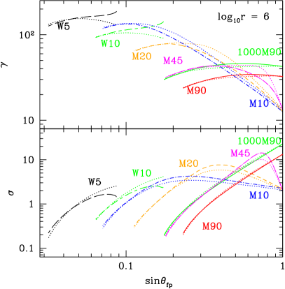
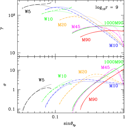
Figure 10.— Dependence of $\gamma$ (upper panels) and $\sigma$ (lower panels) as a function of $\sin\theta_{\rm fp}$ at $r=10^{6}$ (left panels) and $r=10^{9}$ (right panels) for a series of models. The names of the models are indicated next to the corresponding curves. Dotted lines show the analytic solution (49) and other lines show the simulation results. For models with a constant density profile $\rho(\theta_{\rm fp})$ on the star (M90, 1000M90), the analytic approximation works very well at all distances $r$ and all polar angles. For models with a variable angular profile of density on the surface of the star (M45, M20, M10), the agreement is excellent along the field lines for which the initial density is constant; for other field lines, the agreement is less perfect, indicating the best-fit values of the factor $C_{1}$ in equation (48) are different for different field lines. For models with the wall (W10, W5), the agreement is good near the axis and poor near the wall.

We have also performed a simulation called 1000M90 that has a uniform density profile on the stellar surface $\rho(\theta_{\rm fp})=\rho_{0}$ with the same density at $\theta_{\rm fp}=0$ as model M45. Thus, models 1000M90 and M45 have similar profiles of density and $\mu$ near the pole, but they differ near the equator. We expect the two simulations to show nearly identical behavior for polar field lines. This is indeed confirmed, as seen in Fig. 10. The point of this model is to verify that models with variable density, e.g., equation (12), give reliable results near the axis, independent of how we modify the mass-loading of equatorial field lines. The numerical results confirm that this is indeed so.

Figure 10 shows transversal cuts through each of our models at distances of $10^{6}$ and $10^{9}$, and compares the simulation results with the analytic approximation (49) described in §5.3. For models with a constant density profile $\rho(\theta_{\rm fp})$ on the star, the analytic approximation works extremely well at all distances $r$ and all polar angles. For models with a variable angular profile of density on the surface of the star, the agreement is excellent along the field lines originating in the constant-density core while for other field lines, the best-fit values of factor $C_{1}$ in equation (48) apparently varies from one field line to the next. Therefore, adopting a single value $C_{1}=2$ provides only a rough description of acceleration along these field lines.

6. Discussion

A number of previous authors have noted that efficient acceleration of a cold MHD wind requires field lines to diverge away from the equatorial plane. This field geometry was identified as a “magnetic nozzle” due to the geometric similarity of jet nozzles intended to launch a supersonic flow.

We generalized the concept of the “magnetic nozzle” by showing that the geometric bunching of field lines generally induces efficient conversion of magnetic to kinetic energy in neighboring regions. We clarified how this generalized “magnetic nozzle” operates differently for equatorial and polar field lines. Near the midplane, lines merely have to diverge uniformly away from the equator. The more they diverge, the larger the acceleration. For polar field lines, however, what is needed is neither simple divergence nor convergence, but differential bunching or a region that accumulates flux. A particular field line may either converge or diverge relative to its initial (purely radial) configuration. This has no effect on acceleration along this line. However, if neighboring field lines move such that the field strength decreases away from the rotation axis, e.g., as per the simple prescription given in equation (29), then acceleration will occur along the reference field line. The more the differential bunching (i.e., the larger the value of $\xi$ or $\Phi_{0}$), the larger the acceleration.

The rearrangement of field lines described above requires different regions of the magnetosphere to communicate with one another, which is possible only if the flow speed is not too large. This introduces the second major difference between equatorial and polar field lines. Equatorial field lines lose communication once their flow velocities cross the fast magnetosonic speed. This happens when the Lorentz factor $\gamma\sim\mu^{1/3}$, where $\mu$ is the conserved energy flux per unit mass flux along the line. Equivalently, $\gamma\sim\sigma^{1/2}$, where $\sigma$ is the local magnetization parameter. For highly relativistic flows, $\mu$ is very large (e.g., $\mu\sim 10^{6}$ for the Crab Pulsar), so $\gamma$ is much less than $\mu$ at the fast magnetosonic transition. Correspondingly, $\sigma\sim\mu^{2/3}$ is very large, which means that most of the energy flux is still carried as Poynting flux rather than as mass energy flux.

For equatorial field lines beyond the fast point, a small amount of further acceleration is possible, but this only gives an additional logarithmic factor (Beskin et al., 1998). After allowing for this factor, the final asymptotic Lorentz factor on an equatorial field line at a large distance from the star is only $\gamma_{\mathrm{asym}}\sim 2\mu^{1/3}\ln^{1/3}(\Omega r/\mu^{1/3})$ (see eqs. 42 and 46). This is far smaller than the maximum Lorentz factor one would obtain if we had efficient acceleration along the field line, viz., $\gamma_{\rm max}=\mu$. Thus, we confirm the previously known result that equatorial field lines in monopole geometry suffer from a serious $\sigma$ problem. We do not yet see any way of avoiding this conclusion.

The situation is different for polar field lines. Even beyond the fast magnetosonic point, the fluid on these field lines can maintain communication with the axis (where field bunching allows efficient energy conversion). In fact, communication is lost only when $\gamma\sim\sigma^{1/2}/\sin\theta_{j}$, where $\theta_{j}$ is the angle between the poloidal component of the magnetic field and the rotation axis. For small values of $\theta_{j}\sim 0.01-0.1$, as might be appropriate for relativistic jets, this gives a large increase in the asymptotic Lorentz factor reached by the flow. Including the additional gain from the logarithmic factor, we estimate (c.f. eqs. 42 and 48)

$$\gamma_{\mathrm{asym}}\approx(\mu-\gamma_{\mathrm{asym}})^{1/3}\frac{C_{1}\ln^{1/3}(\Omega r\sin^{5/3}\theta_{j,c}/\mu^{1/3})}{\sin^{2/3}\theta_{j,c}},$$ (50)

or, using (11),

$$\gamma_{\mathrm{asym}}\approx\sigma^{1/2}\frac{C_{1}^{3/2}\ln^{1/2}(\Omega r\sin^{5/3}\theta_{j,c}/\mu^{1/3})}{\sin\theta_{j,c}},$$ (51)

where we note that $\mu-\gamma_{\mathrm{asym}}\propto\sigma\propto\sin^{2}\theta_{j,c}$ near the rotation axis. In the limit $\sigma\gg 1$ we can simplify (50) by approximating $\mu-\gamma_{\mathrm{asym}}\approx\mu$. These expressions are applicable beyond the causality surface as approximately given by equation (42). As an order of magnitude estimate, in these formulae one could substitute $\theta_{\rm fp}$, $\theta$, or $\theta_{j}$ in place of $\theta_{j,c}$. In any case, the $\sin\theta_{j,c}$ factors in the denominator of equations (51) and (50) indicate that $\gamma_{\mathrm{asym}}$ is larger near the poles.

6.1. Collimation and Acceleration

Equations (40), (51) predict that at roughly the same value of $\sigma\sim 1$, an asymptotically more collimated simulation reaches a larger Lorentz factor:

$$\gamma_{\mathrm{asym}}\propto\frac{1}{\sin\theta_{j,c}},$$ (52)

where $\theta_{j,c}\sim\theta_{\rm fp}\gtrsim\theta_{j}$ is the angle at the causality surface. Figure 10 confirms this for the sequence of models M45–M20–M10, all of which have the same maximum value of $\mu$, $\mu_{\rm max}=460$. If all of these models could convert all of the electromagnetic energy flux into kinetic energy flux, each of them would reach the maximum energetically allowed Lorentz factor, $\gamma=\mu_{\rm max}$. While such a full conversion does not happen in any of these models, more collimated models reach higher Lorentz factors, in agreement with equation (52): each subsequent model in the sequence of models M45–M20–M10 is roughly twice as collimated as the previous one and at $r=10^{9}$ attains approximately twice as large a Lorentz factor, $50$–$95$–$170$.

6.2. Application to Relativistic Jets and GRBs

The net conclusion of the previous discussion is that, whereas there is indeed a serious $\sigma$ problem for pulsar winds, there is no similar problem for relativistic jets. We show that even if a flow is unconfined and has a monopolar-like shape, it can still efficiently accelerate in the polar region. For a jet angle $\theta_{j}\sim 2^{\circ}$, for instance, the scaling (51) predicts an asymptotic Lorentz factor $\gamma_{\mathrm{asym}}>100$ if the jet efficiently converts electromagnetic to kinetic energy and reaches $\sigma\sim 1$. In fact, if the jet is not efficient and carries more of its energy as Poynting flux (e.g. for a larger value of $\mu$, see eqs. 51–50), then $\sigma>1$, and we will have even larger values of $\gamma_{\mathrm{asym}}$. These estimates are confirmed by the numerical simulations described in this paper.

The inferred total power of long GRBs is on the order of $10^{51}$ erg (Piran, 2005; Meszaros, 2006; Liang et al., 2008); however, much less energetic events, with total energy release as low as $10^{48}$ erg, have also been observed (Soderberg et al., 2004, 2006). Let us compute the power output of jets in our numerical models and make sure that our jets are energetic enough to be consistent with these observations. The total power coming out from the compact object surface within the low-density core, $\theta<\theta_{\rm max}$, is

$$P^{\rm jet} = \int\limits_{0}^{\theta_{\rm max}}2\pi r^{2}d\theta\sin\theta\,S(r,\theta)|_{r=1}\approx\frac{\Omega^{2}}{2}\int\limits_{0}^{\theta_{\rm max}}d\theta\sin^{3}\theta$$ (53)

$$= \frac{\Omega^{2}}{2}\times\frac{4(2+\cos\theta_{\rm max})}{3}\times\sin^{4}\frac{\theta_{\rm max}}{2}\approx\frac{\Omega^{2}}{8}\,\theta_{\rm max}^{4},$$

where the last equality is for $\theta_{\rm max}\ll 1$. Converting the result to physical units, we obtain

$$P^{\rm jet}\approx\frac{1}{8}\Omega^{2}B_{r}^{2}r_{0}^{4}\theta_{\rm max}^{4}/c,$$ (54)

where $B_{r}$ is the value of radial magnetic field component on the surface of the compact object and $r_{0}$ is the compact object radius. Evaluating the jet power for a magnetar with a characteristic period $P=1$ ms and a surface magnetic field of $10^{15}$ G, we get

$$P^{\rm jet}_{\rm NS} \approx 2\times 10^{47}\left[\frac{\mathrm{erg}}{\mathrm{s}}\right]$$ (55)

$$\times \left(\frac{1\mathrm{ms}}{P}\right)^{2}\left(\frac{B_{r}}{10^{15}\mathrm{G}}\right)^{2}\left(\frac{r_{0}}{10\mathrm{km}}\right)^{2}\left(\frac{\theta_{\rm max}}{10^{\circ}}\right)^{4}.$$

For a maximally-spinning black hole with dimensionless spin parameter $a=1$, mass $3M_{\odot}$, and surface magnetic field strength $10^{16}$ G (McKinney, 2005), we have

$$P^{\rm jet}_{\rm BH}\approx 5\times 10^{48}\,a^{2}\left(\frac{B_{r}}{10^{16}\mathrm{G}}\right)^{2}\left(\frac{M}{3M_{\odot}}\right)^{2}\left(\frac{\theta_{\rm max}}{10^{\circ}}\right)^{4}\left[\frac{\mathrm{erg}}{\mathrm{s}}\right].$$ (56)

Given a characteristic duration of $10$–$100$ seconds for a long GRB, our numerical jets provide, for the black hole case, $10^{50}$–$10^{51}$ erg per event for model M10, $10^{51}$–$10^{52}$ erg for M20, and $10^{52}$–$10^{53}$ erg for M45. Therefore, the simulated jets from black holes in models M10 and M20 are energetic enough and move at sufficiently high Lorentz factors ($\gamma\gtrsim 100$) to account for most long GRBs and can certainly account for low luminosity events. The energetics is also right for short GRBs: the simulated jets output $10^{49}$–$10^{50}$ erg during a characteristic event duration of $1$ second (Nakar, 2007). For the magnetar case the energetics is lower: $10^{47}$–$10^{48}$–$10^{50}$ erg/s for a sequence of models M10–M20–M45. Therefore, the simulated jets from magnetars can account for less-luminous long GRB events and most short GRBs.

While the energy fraction in the polar jet is small as compared to the total energy extracted by magnetic fields from the black hole, $P^{\rm jet}/P^{\rm tot}\sim\theta_{\rm max}^{4}$ (eq. 54, which assumes a uniform magnetic field distribution at the BH horizon), the absolute value of jet power $P^{\rm jet}$ is sufficiently large to account for long and short GRBs. We point out that the magnetic flux in accreting black hole systems is non-uniformly concentrated in the polar region of the BH (e.g., McKinney, 2005, due to ambient pressure of the accretion flow), and therefore the total energy losses of the spinning black hole are actually dominated by the losses from the polar region rather than from the midplane region, meaning a larger fraction of power in the jet than given by eq. (54).

A very interesting question is whether the models suggest any characteristic value for the quantity $\gamma_{j}\theta_{j}$: is this quantity generally smaller or larger than unity? For a jet with $\gamma_{j}\theta_{j}\gg 1$ (say, $\sim 10$) only part of the jet within the beaming angle $\theta_{b}\approx 1/\gamma_{j}\ll\theta_{j}$ is visible to a remote observer. As the interaction with the ambient medium decelerates the jet and the beaming angle becomes comparable to the jet opening angle, the edges of the jet come into sight and the light curve steepens achromatically, displaying a “jet break” (Piran, 2005; Meszaros, 2006). In the other limit, $\gamma_{j}\theta_{j}\ll 1$, a jet would be incapable of producing achromatic breaks in GRB light curves.

Achromatic breaks have been found in pre-Swift times (Frail et al., 2001; Bloom et al., 2003; Zeh et al., 2006) and have yielded $\theta_{j}\sim 0.03$–$1$ rad. The situation is quite different in the post-Swift times for which a large amount of data available, and no jet breaks have been found to fully satisfy closure relations in all bands (Liang et al., 2008). However, if one or more of the closure relations are relaxed, some of the breaks may be interpreted as “achromatic” and be used to derive jet opening angles that span a similar range as pre-Swift GRBs (Liang et al., 2008). Overall, it appears that the Lorentz factor of most GRBs is $\gamma_{j}\gtrsim 100$ (Piran 2005; Meszaros 2006, up to $\sim 400$, Lithwick & Sari 2001) which, with the above estimates for $\theta_{j}$, gives $\gamma_{j}\theta_{j}\gtrsim 3$ and indicates that in principle achromatic jet breaks are possible.

Our numerical models have $\gamma_{j}\theta_{j}\sim 5$–$15$, where the index $j$ denotes quantities evaluated at the jet boundary which we define as the boundary of matter-dominated region $\sigma<1$. In this respect it is particularly fruitful to compare simulations M10 and W10. As we discussed in §5.4, the wall in model W10 prevents field lines from collapsing onto the pole as much as they do in model M10. Comparison of field lines with $\sigma\sim 1$ for these models (see Figs. 7 and 8), reveals a difference in the Lorentz factor of at most $20$% and a much larger difference in the value of $\gamma_{j}\theta_{j}$ (caused by a large difference in $\theta_{j}$ due to the effect of the wall): $\gamma_{j}\theta_{j}\approx 5$ for M10 and $\approx 12$ for W10. The most collimated model W5 produces an even larger value, $\gamma_{j}\theta_{j}\approx 15$.

We now analytically confirm that in general the quantity $\gamma_{j}\theta_{j}\sim 5$–$10$. For the jet boundary, using (51) and characteristic values $\Omega\sim 1$, $\theta_{j,c}\sim 0.04$–$0.4$, $\mu\sim 10^{3}$, $r\sim 10^{6}$–$10^{9}$, $\theta_{j}/\theta_{j,c}\sim 0.5$–$1$ (see Figs. 7, 8, and 9), we get:

$$\gamma_{j}\theta_{j}\sim\frac{4\theta_{j}}{\theta_{j,c}}\sigma^{1/2}\log_{10}^{1/2}\left(\frac{r}{10^{2}{\!-\!}10^{3}}\right)\sim(4{\!-\!}10)\sigma^{1/2}$$ (57)

which is in good agreement with the simulation results. The large value of $\gamma_{j}\theta_{j}$ in this analysis arises solely due to the logarithmic factor that appears because a significant fraction of the acceleration occurs after crossing the causality surface, in the inefficient acceleration region: this is the case for all unconfined flows studied in our paper. This should be contrasted with confined outflows, collimated by walls with prescribed shapes, for which most of the acceleration tends to complete before crossing the causality surface and which have $\gamma_{j}\theta_{j}\sim 1$ (Komissarov et al., 2009). We note that if we do not require that jets are matter-dominated, e.g. we allow $\sigma>1$ as in Lyutikov & Blandford’s (2003) model of GRBs, then the value of $\gamma_{j}\theta_{j}$ will be even higher (see eq. 57).

According to equation (57), we can attribute the fact that some post-Swift GRBs show quasi-achromatic jet breaks, while many do not, by associating the former with jets that have $\gamma_{j}\theta_{j}>1$ and the latter with those that have $\gamma_{j}\theta_{j}<1$. Such a scatter in $\gamma_{j}\theta_{j}$ might be naturally produced by differences in GRB environment (affecting $\theta_{j}/\theta_{j,c}$, see eq. 57) or the properties of the central engine (affecting $\sigma$). Indeed, according to (57), a low value of $\sigma$ ($\ll 1$) or $\theta_{j}$ ($\ll\theta_{j,c}$) in our jets would mean $\gamma_{j}\theta_{j}<1$ and so the absence of a jet break.

One could use equation (50), which is based upon our analytical model of the simulations, to obtain the Lorentz factor of any GRB jet. If the black hole or neutron star is nearly maximally spinning with $\Omega\sim 0.25$ and has a polar region with the reasonable value of $\mu\sim 1000$ (TMN08), and if we consider an opening angle $\theta_{j}\sim 4^{\circ}$, then by $r\sim 10^{8}\sim 10^{14}$ cm one obtains $\gamma_{j}\sim 250$ and $\gamma_{j}\theta_{j}\sim 17$. For a range of opening angles with sufficient luminosity, one obtains a range of Lorentz factors consistent with both short and long duration GRB jets (Piran, 2005; Meszaros, 2006). Further, the product $\gamma_{j}\theta_{j}\gtrsim 1$, indicating an afterglow can exhibit the so-called “achromatic jet breaks,” where observations imply $\gamma_{j}\theta_{j}\gtrsim 3$ for long-duration GRB jets (Piran, 2005; Meszaros, 2006). Our simulations and analytical models have $\gamma_{j}\theta_{j}\sim 5{-}15$, which is proof of principle that magnetically-driven jets can produce jet breaks.

7. Conclusions

We have studied relativistic magnetized winds from rapidly rotating compact objects endowed with a split-monopole magnetic field geometry. We used the relativistic MHD code, HARM, to simulate these outflows. We have constructed analytical approximations to our simulations that describe fairly accurately the Lorentz factor and the efficiency of magnetic energy to kinetic energy conversion in the outflow.

Our main result is that, contrary to conventional expectations, the winds from compact objects endowed with monopole magnetic fields have efficient conversion of magnetic energy to kinetic energy near the rotation axes. We identify this polar wind as a jet since it contains a sufficiently high luminosity within the required opening angles of several degrees, and it accelerates to ultrarelativistic Lorentz factors through an efficient conversion of magnetic energy to kinetic energy ($\gamma\sim\mu$ and $\sigma<1$ at large radii). We note that Lyubarsky & Eichler (2001) have identified a similar polar jet in unconfined magnetospheres based on its relative degree of collimation to the rest of the flow and the relativistic Lorentz factor. However, they did not concentrate on the acceleration efficiency and the transition to the matter-dominated flow. One can use equation (50) to show that, for example, order unity solar mass black holes or neutron stars with $\mu\approx\sigma\sim 300$ near the compact object will readily produce $\gamma_{j}\sim 150$ at $10^{14}$ cm with $\theta_{j}\sim 4^{\circ}$ such that $\gamma_{j}\theta_{j}\sim 10$.

We are able to analytically explain how the jet efficiently converts magnetic energy to kinetic energy by identifying a “causality surface,” beyond which the jet can no longer communicate with the rotation axis that contains the flux core. When one region of the jet can no longer communicate to the flux core, that region ceases to accelerate efficiently. The communication between the jet body and the rotation axis allows magnetic flux surfaces and the Poynting flux associated with them to become less concentrated in the main body of the jet (at the expense of the bunch-up near the axis), and it is this process that allows efficient conversion of magnetic to kinetic energy (§4.3). A similar mechanism, called “magnetic nozzle,” was first described in Begelman & Li (1994). We clarify this mechanism by showing that the accumulation of flux near the rotation axis leads to a stronger decrease in $\sigma$ for polar field lines than for equatorial field lines. This effect is a new feature of ideal MHD winds that has not been discussed by Begelman & Li (1994) or any other authors except the very recent work by Komissarov et al. (2009).

Our results demonstrate that ultrarelativistic jet production is a surprisingly robust process and probably requires less fine-tuning than previously thought. It is possible for spinning black holes and neutron stars to produce ultrarelativistic jets even without the presence of an ambient confining medium to collimate the jet. Further, we show that even unconfined (or weakly confined) winds from compact objects can produce sufficiently energetic jets ($L_{j}\sim 10^{49}$ erg/s) to explain many long GRBs and most short GRBs.

We have confirmed the standard result that monopole magnetospheres are inefficient accelerators in the equatorial region. We have thus been unable to solve the $\sigma$-problem for the Crab PWN under the assumption of an ideal MHD axisymmetric flow from a star endowed with a split-monopole magnetosphere. We note that at some distance from the neutron star an ideal MHD approximation may break down (Usov, 1994; Lyutikov & Blackman, 2001). No highly relativistic jet is observed in the Crab and Vela PWNe, despite our results that suggest there should be such a feature. There are observations of non-relativistic jets with $v/c\sim 0.5$ that appear diffuse and borderline stable. One way to resolve this discrepancy is that in PWNe systems the axisymmetric ultrarelativistic jets we find are unstable to non-axisymmetric perturbations and so can be a prodigious source of high-energy particles and radiation via dissipation that causes the jet to slow to non-relativistic velocities (e.g., Giannios et al., 2009). This notion of a visible jet emerging directly from the pulsar (Lyubarsky & Eichler, 2001) is an alternative model to the more recent view that the observed jet is caused by a post-shock polar backflow with $\sigma\gtrsim 0.01$ that is guided by hoop stresses and forced to converge toward (and rise up along) the rotation axis (Komissarov & Lyubarsky, 2004; Del Zanna et al., 2004). In either model, one must consider non-axisymmetric instabilities since, in the backflow model, the shock structure and backflow could be highly non-axisymmetric and potentially unstable to non-axisymmetric instabilities.

We remark that while preparing this paper for publication, Komissarov et al. (2009) posted a paper describing ideal MHD simulations of confined and unconfined winds. They do make a minor note that their simulations of unconfined monopole outflows show efficient conversion of magnetic energy to kinetic energy near the rotation axis. We find similar results to theirs for the unconfined monopole wind. We are further able to make analytical estimates that explain the nature of this efficient conversion via introducing a causality surface at which the jet loses causal connection with the polar axis. We are also able to obtain a closed-form approximation for the Lorentz factor in this region based upon a precise notion of the “causality surface.” We note that previous authors who studied stars endowed with a split-monopole field geometry in the ideal MHD approximation (Bogovalov, 2001; Bucciantini et al., 2006) did not perform simulations to large enough radii in order to observe the outflow achieving such an efficient conversion of magnetic to kinetic energy near the rotation axis or reaching such large Lorentz factors.

We conclude with prospects for future research. Our solutions are axisymmetric, assume the compact object is endowed with a monopolar field geometry, assume particles are injected with $\gamma\sim 1$ near the compact object, assume $\sigma\gg 1$ near the equatorial plane, and assume the ideal cold MHD approximation holds. In future work we plan to consider the stability of our solutions to non-axisymmetric instabilities (c.f. Narayan et al., 2009), the effect of external confinement leading to highly-collimated solutions, the injection of ultrarelativistic particles as suggested to occur, e.g., in the Crab pulsar, the injection of non-relativistic particles as may be relevant for thin disks (Bogovalov & Tsinganos, 1999), and the effect of $\sigma\sim 0$ near the equatorial plane as required near the pulsar’s equatorial current sheet or for any system with an accretion disk.

Appendix A Lorentz factor in an ideal MHD flow

In this section we derive an approximate expression for the Lorentz factor in an ideal MHD flow. Conservation of energy and angular momentum flux along a field line imply (e.g., Contopoulos & Kazanas, 2002):

$$\gamma(1-\Omega Rv_{\varphi})=\gamma_{0},$$ (A1)

where $\Omega$ is the angular frequency of field line and $\gamma_{0}$ and $\gamma$ are the initial and the local Lorentz factors of the field line,

$$\gamma=(1-v_{p}^{2}-v_{\varphi}^{2})^{-1/2}.$$ (A2)

For convenience, introduce auxiliary variables $x=\Omega R$ and $y$:

$$E = xB_{p},$$ (A3)

$$B_{\varphi} = -yB_{p}.$$ (A4)

The drift Lorentz factor (14) is

$$\gamma_{\rm dr}^{2}=\frac{B^{2}}{B^{2}-E^{2}}=\frac{1+y^{2}}{1+y^{2}-x^{2}}.$$ (A5)

Resolving (1), (A1)–(A4) for $\gamma$, we obtain:

$$\gamma^{2}=\frac{\left[\gamma_{0}^{2}\left(1+y^{2}\right)+x^{2}y^{2}\right]^{2}}{\left(1+y^{2}-x^{2}\right)\left[xy(x^{2}+\gamma_{0}^{2}-1)^{1/2}+\gamma_{0}(1+y^{2}-x^{2})^{1/2}\right]^{2}}.$$ (A6)

This equation is exact and expresses the MHD fluid velocity via the local parameters ($x$, $y$) and the footpoint parameters ($\gamma_{0}$). In the limit $x\gg 1$, we have the following analytic approximation for the MHD Lorentz factor (assuming that $\left|B_{\varphi}\right|\approx E$, or that $y^{2}-x^{2}\ll x^{2}$),

$$\gamma_{a}^{2}=\frac{\gamma_{0}^{2}+x^{2}}{1+y^{2}-x^{2}},$$ (A7)

that is very close to the drift Lorentz factor (A5). This shows that asymptotically the Lorentz factor of the MHD flow (A6) is closely approximated by the drift Lorentz factor (A5) (c.f. Beskin et al., 1998, 2004; Vlahakis, 2004). We note that another convenient, albeit slightly less accurate, form of (A7) is

$$\gamma_{a}^{2}\approx\gamma_{0}^{2}-1+\gamma_{\rm dr}^{2}.$$ (A8)

As we show by comparison to numerical results, formula (A7) works extremely well not only asymptotically but at all distances from the star. We now show analytically why this is the case. In the monopole flow $\left|B_{\varphi}\right|\approx E$ at all distances from the star (see §4.1), therefore neglecting $y^{2}-x^{2}$ as compared to $x^{2}$, we obtain:

$$\frac{\gamma}{\gamma_{a}}\approx\frac{\gamma_{0}^{2}(1+x^{2})+x^{4}}{(\gamma_{0}^{2}+x^{2})^{1/2}\left[\gamma_{0}+x^{2}(\gamma_{0}^{2}+x^{2}-1)^{1/2}\right]}.$$ (A9)

According to this equation, the relative deviation of $\gamma_{a}$ w.r.t. $\gamma$ is always smaller than $6$% for any $x\equiv\Omega R$ and $\gamma_{0}$. Therefore, formula (A7) can be used as an accurate approximation for the MHD fluid Lorentz factor at all distances from the star and initial Lorentz factor $\gamma_{0}$.

We now recast the approximation to the Lorentz factor $\gamma_{a}$ (A7) in a two-component form (c.f. TMN08, ):

$$\frac{1}{\gamma^{2}}\approx\frac{1}{\gamma_{1}^{2}}+\frac{1}{\gamma_{2}^{2}},$$ (A10)

where

$$\gamma_{1}^{2}=\gamma_{0}^{2}+x^{2}=\gamma_{0}^{2}+(\Omega R)^{2}$$ (A11)

increases roughly linearly with distance and

$$\gamma_{2}^{2}\approx\frac{x^{2}}{y^{2}-x^{2}}=\frac{E^{2}}{B_{\varphi}^{2}-E^{2}}$$ (A12)

is related to the poloidal radius of curvature of the field line $R_{c}$ (TMN08) in the limit $\gamma_{2}\ll\mu$:

$$\gamma_{2}^{2}\approx C\frac{R_{c}}{R}\cos\theta$$ (A13)

where $C\simeq 1$ is a numerical factor. Since $\gamma^{2}/2$ is the harmonic mean of $\gamma_{1}^{2}$ and $\gamma_{2}^{2}$, the smaller of $\gamma_{1}$ and $\gamma_{2}$ determines the total Lorentz factor. Close to the compact object the first term in (A10) dominates, and $\gamma$ increases roughly linearly with distance from the axis (see §5.2 and TMN08),

$$\gamma\approx\gamma_{1}=\left[\gamma_{0}^{2}+(\Omega R)^{2}\right]^{1/2}\approx\Omega R.$$ (A14)

As we discuss in §5.2, beyond the causality surface the second term in (A10) becomes dominant and there the Lorentz factor grows logarithmically,

$$\gamma\approx\gamma_{2}\propto\ln^{1/3}r.$$ (A15)

In the next section we present a compact derivation of this result.

Appendix B Logarithmic acceleration regime

In this section we consider acceleration along near-midplane field lines, which have $\theta^{\prime}=\pi/2-\theta\ll 1$, and show that it is logarithmic sufficiently far from the central star where the flow has switched to the second acceleration regime (A13). We limit ourselves to a highly magnetized region of the flow, $\gamma\ll\mu$. Assuming a near-monopolar structure in this region, we express the rate of change of angle $\theta^{\prime}$ along a field line in terms of its local poloidal curvature radius $R_{c}$ as

$$\frac{d\theta^{\prime}}{dr}\approx\frac{1}{R_{c}}{\approx}\frac{C\theta^{\prime}}{r\gamma^{2}},$$ (B1)

where in the latter equality we used equation (A13) and the fact that $r\approx R$ for $\theta^{\prime}\ll 1$. Differentiating equation (25), we express $d\gamma/d\theta^{\prime}$ along the field line:

$$\frac{d\gamma}{d\theta^{\prime}}\approx\mu\frac{\theta^{\prime}_{\rm fp}}{(\theta^{\prime})^{2}}.$$ (B2)

Combining equations (B1) and (B2) and assuming a near-monopolar structure, $\theta^{\prime}\approx\theta^{\prime}_{\rm fp}$, we obtain a differential equation for $\gamma$:

$$\frac{\gamma^{2}d\gamma}{\mu}\approx C\frac{dr}{r},$$ (B3)

or

$$\gamma\approx(C\mu)^{1/3}\ln^{1/3}(r/r_{*}),$$ (B4)

where $r_{*}$ is an integration constant. In §5.3 we argue that $r_{*}\approx r_{c}$, the radius at which the field line intersects the causality surface.

Appendix C Auxiliary approximate analytic solution

HARM integrates the ideal cold MHD equations of motion by first interpolating the primitive quantities (i.e. density, velocity, and magnetic field) from cell centers to cell faces. The cell faces will generally now have two values corresponding to an interpolation from different cell centers. As described in Gammie et al. (2003), these two values are used to compute a generally dissipative flux that is used to advance the set of conserved quantities forward in time. These conserved quantities are then inverted to produce the new primitive quantities.

In cases where one roughly knows the solution for the primitive quantities as functions of position, one can instead interpolate the ratio of the primitive quantities to the estimated solution. This reduces numerical dissipation by reducing the difference in the two values of primitive quantities interpolated to the face. The closer the estimated solution is to the true solution, the lower the numerical dissipation. So it is useful to estimate the solution as best one can. The particular form of this estimated solution has no other effect on the numerical simulation.

Here we provide our estimated solution based upon an approximate extension of known force-free solutions (TMN08):

$$B_{r} = r^{-2},$$ (C1)

$$B_{\theta} = 0,$$ (C2)

$$B_{\varphi} = -\Omega RB_{r},$$ (C3)

$$\frac{1}{\gamma^{2}-\gamma_{0}^{2}} = \frac{1}{(\Omega R)^{2}}+\frac{1}{(\mu/2)^{2}},$$ (C4)

$$u_{r}^{2} = \gamma^{2}-1,$$ (C5)

$$u_{\theta} = 0,$$ (C6)

$$u_{\varphi} = \frac{\gamma\Omega RB_{r}^{2}}{B_{r}^{2}+B_{\varphi}^{2}},$$ (C7)

$$\rho = \eta\frac{B_{r}}{u_{r}},$$ (C8)

with vectors given in an orthonormal (physical) basis and where $\eta$ is given by the boundary conditions according to equation (4). We interpolate the numerical solution (given in a contravariant coordinate basis) divided by the estimated solution (also in a contravariant coordinate basis), with the exception of $B_{\theta}$ and $u_{\theta}$ for which we do not divide by the analytic solution. In addition, we independently interpolate $\gamma$ using equation (C4) in order to rescale the interpolated 4-velocity, which leads to a more accurate solution (Tchekhovskoy et al., 2007).

Appendix D Mach Cone for Fast Magnetosonic Waves

In this section we derive the expression for the half-opening angle of a Mach cone for fast magnetosonic waves. Consider a segment of the relativistic magnetized wind propagating with a velocity vector $\vec{v}$ and Lorentz factor $\gamma$. Let a fast magnetosonic wave travel in the comoving fluid frame at an angle $\xi^{\prime}$ to the direction $\vec{v}$. Decomposing the wave velocity into parallel and perpendicular components, we have

$$v^{\prime}_{\parallel}=v_{f}\cos\xi^{\prime},\qquad v{{}^{\prime}}_{\perp}=v_{f}\sin\xi^{\prime}.$$ (D1)

Transforming back to the lab frame, the components of the wave velocity become

$$v_{\parallel}=\frac{v_{f}\cos\xi^{\prime}+v}{(1+vv_{f}\cos\xi^{\prime})},\qquad v_{\perp}=\frac{v_{f}\sin\xi^{\prime}}{\gamma(1+vv_{f}\cos\xi^{\prime})}.$$ (D2)

Therefore, in the lab frame, the wave velocity vector is oriented at an angle $\xi$ to the vector $\vec{v}$, where

$$\tan\xi=\frac{v_{\perp}}{v_{\parallel}}=\frac{v_{f}\sin\xi^{\prime}}{\gamma(v_{f}\cos\xi^{\prime}+v)}.$$ (D3)

In the lab frame, different waves have different values of $\xi$. Assuming that the medium moves with a superfast speed (i.e., $v>v_{f}$), all waves move in the downstream direction in the lab frame and their $\xi$ values are all less than a certain maximum $\xi_{\rm max}$. To determine $\xi_{\rm max}$, we maximize $\tan\xi$ with respect to variations of $\xi^{\prime}$. The maximum is achieved when

$$\cos\xi^{\prime}=-\frac{v_{f}}{v},\qquad\sin\xi^{\prime}=\frac{\sqrt{v^{2}-v_{f}^{2}}}{v}.$$ (D4)

This gives the half-opening angle of the Mach cone, $\xi_{\rm max}$:

$$\tan\xi_{\rm max} = \frac{v_{f}}{\gamma\sqrt{v^{2}-v_{f}^{2}}},$$ (D5)

$$\sin\xi_{\rm max} = \frac{\gamma_{f}v_{f}}{\gamma v}=\frac{1}{M_{f}}.$$ (D6)

References

- Appl & Camenzind (1993) Appl, S. & Camenzind, M. 1993, A&A, 274, 699
- Arons (1983) Arons, J. 1983, ApJ, 266, 215
- Balbus & Hawley (1998) Balbus, S. A. & Hawley, J. F. 1998, Reviews of Modern Physics, 70, 1
- Barkov & Komissarov (2008) Barkov, M. & Komissarov, S. 2008, preprint (arXiv:0801.4861)
- Begelman (1998) Begelman, M. C. 1998, ApJ, 493, 291
- Begelman & Li (1994) Begelman, M. C. & Li, Z.-Y. 1994, ApJ, 426, 269
- Beskin (1997) Beskin, V. S. 1997, Soviet Physics Uspekhi, 40, 659
- Beskin et al. (1998) Beskin, V. S., Kuznetsova, I. V., & Rafikov, R. R. 1998, MNRAS, 299, 341
- Beskin & Nokhrina (2006) Beskin, V. S. & Nokhrina, E. E. 2006, MNRAS, 367, 375
- Beskin & Nokhrina (2008) —. 2008, preprint (arXiv:0810.4307)
- Beskin et al. (2004) Beskin, V. S., Zakamska, N. L., & Sol, H. 2004, MNRAS, 347, 587
- Blandford (1976) Blandford, R. D. 1976, MNRAS, 176, 465
- Blandford & Payne (1982) Blandford, R. D. & Payne, D. G. 1982, MNRAS, 199, 883
- Blandford & Znajek (1977) Blandford, R. D. & Znajek, R. L. 1977, MNRAS, 179, 433
- Bloom et al. (2003) Bloom, J. S., Frail, D. A., & Kulkarni, S. R. 2003, ApJ, 594, 674
- Bogovalov & Tsinganos (1999) Bogovalov, S. & Tsinganos, K. 1999, MNRAS, 305, 211
- Bogovalov (1995) Bogovalov, S. V. 1995, Astronomy Letters, 21, 565
- Bogovalov (2001) —. 2001, A&A, 371, 1155
- Bucciantini et al. (2006) Bucciantini, N., Thompson, T. A., Arons, J., Quataert, E., & Del Zanna, L. 2006, MNRAS, 368, 1717
- Camenzind (1986) Camenzind, M. 1986, A&A, 162, 32
- Camenzind (1987) —. 1987, A&A, 184, 341
- Camenzind (1989) Camenzind, M. 1989, in Astrophysics and Space Science Library, Vol. 156, Accretion Disks and Magnetic Fields in Astrophysics, ed. G. Belvedere, 129–143
- Catlett et al. (2007) Catlett, C., Andrews, P., Bair, R., et al. 2007, HPC and Grids in Action, Amsterdam
- Chandrasekhar (1956) Chandrasekhar, S. 1956, ApJ, 124, 232
- Cheng et al. (1976) Cheng, A., Ruderman, M., & Sutherland, P. 1976, ApJ, 203, 209
- Cheng et al. (1986) Cheng, K. S., Ho, C., & Ruderman, M. 1986, ApJ, 300, 522
- Cheng et al. (2000) Cheng, K. S., Ruderman, M., & Zhang, L. 2000, ApJ, 537, 964
- Chiueh et al. (1991) Chiueh, T., Li, Z.-Y., & Begelman, M. C. 1991, ApJ, 377, 462
- Chiueh et al. (1998) —. 1998, ApJ, 505, 835
- Contopoulos & Kazanas (2002) Contopoulos, I. & Kazanas, D. 2002, ApJ, 566, 336
- Contopoulos et al. (1999) Contopoulos, I., Kazanas, D., & Fendt, C. 1999, ApJ, 511, 351
- Contopoulos (1995a) Contopoulos, J. 1995a, ApJ, 450, 616
- Contopoulos (1995b) —. 1995b, ApJ, 446, 67
- Coroniti (1990) Coroniti, F. V. 1990, ApJ, 349, 538
- Daugherty & Harding (1982) Daugherty, J. K. & Harding, A. K. 1982, ApJ, 252, 337
- Del Zanna et al. (2004) Del Zanna, L., Amato, E., & Bucciantini, N. 2004, A&A, 421, 1063
- Eichler (1993) Eichler, D. 1993, ApJ, 419, 111
- Emmering & Chevalier (1987) Emmering, R. T. & Chevalier, R. A. 1987, ApJ, 321, 334
- Fendt (1997) Fendt, C. 1997, A&A, 319, 1025
- Fendt et al. (1995) Fendt, C., Camenzind, M., & Appl, S. 1995, A&A, 300, 791
- Fendt & Ouyed (2004) Fendt, C. & Ouyed, R. 2004, ApJ, 608, 378
- Frail et al. (2001) Frail, D. A., Kulkarni, S. R., Sari, R., Djorgovski, S. G., Bloom, J. S., Galama, T. J., Reichart, D. E., Berger, E., Harrison, F. A., Price, P. A., Yost, S. A., Diercks, A., Goodrich, R. W., & Chaffee, F. 2001, ApJ, 562, L55
- Gammie et al. (2003) Gammie, C. F., McKinney, J. C., & Tóth, G. 2003, ApJ, 589, 444
- Giannios et al. (2009) Giannios, D., Uzdensky, D. A., & Begelman, M. C. 2009, MNRAS, 395, L29
- Goldreich & Julian (1969) Goldreich, P. & Julian, W. H. 1969, ApJ, 157, 869
- Goldreich & Julian (1970) —. 1970, ApJ, 160, 971
- Gruzinov (2005) Gruzinov, A. 2005, Physical Review Letters, 94, 021101
- Guderley (1962) Guderley, K. G. 1962, The theory of transonic flow (Oxford, Pergamon Press)
- Heyvaerts & Norman (1989) Heyvaerts, J. & Norman, C. 1989, ApJ, 347, 1055
- Hibschman & Arons (2001a) Hibschman, J. A. & Arons, J. 2001a, ApJ, 554, 624
- Hibschman & Arons (2001b) —. 2001b, ApJ, 560, 871
- Kennel & Coroniti (1984a) Kennel, C. F. & Coroniti, F. V. 1984a, ApJ, 283, 694
- Kennel & Coroniti (1984b) —. 1984b, ApJ, 283, 710
- Kirk & Skjæraasen (2003) Kirk, J. G. & Skjæraasen, O. 2003, ApJ, 591, 366
- Komissarov (2001) Komissarov, S. S. 2001, MNRAS, 326, L41
- Komissarov (2002a) —. 2002a, MNRAS, 336, 759
- Komissarov (2002b) —. 2002b, MNRAS, 336, 759
- Komissarov (2006) —. 2006, MNRAS, 367, 19
- Komissarov et al. (2007) Komissarov, S. S., Barkov, M. V., Vlahakis, N., & Königl, A. 2007, MNRAS, 380, 51
- Komissarov & Lyubarsky (2004) Komissarov, S. S. & Lyubarsky, Y. E. 2004, MNRAS, 349, 779
- Komissarov et al. (2009) Komissarov, S. S., Vlahakis, N., Königl, A., & Barkov, M. V. 2009, MNRAS, 216
- Li et al. (1992) Li, Z.-Y., Chiueh, T., & Begelman, M. C. 1992, ApJ, 394, 459
- Liang et al. (2008) Liang, E.-W., Racusin, J. L., Zhang, B., Zhang, B.-B., & Burrows, D. N. 2008, ApJ, 675, 528
- Lithwick & Sari (2001) Lithwick, Y. & Sari, R. 2001, ApJ, 555, 540
- Lovelace (1976) Lovelace, R. V. E. 1976, Nature, 262, 649
- Lovelace et al. (1986) Lovelace, R. V. E., Mehanian, C., Mobarry, C. M., & Sulkanen, M. E. 1986, ApJS, 62, 1
- Lovelace & Romanova (2003) Lovelace, R. V. E. & Romanova, M. M. 2003, ApJ, 596, L159
- Lovelace et al. (2006) Lovelace, R. V. E., Turner, L., & Romanova, M. M. 2006, ApJ, 652, 1494
- Lyubarsky (2009) Lyubarsky, Y. 2009, preprint (arXiv:0902.3357)
- Lyubarsky & Eichler (2001) Lyubarsky, Y. & Eichler, D. 2001, ApJ, 562, 494
- Lyubarsky & Kirk (2001) Lyubarsky, Y. & Kirk, J. G. 2001, ApJ, 547, 437
- Lyubarsky (2005) Lyubarsky, Y. E. 2005, MNRAS, 358, 113
- Lyutikov & Blackman (2001) Lyutikov, M. & Blackman, E. G. 2001, MNRAS, 321, 177
- Lyutikov & Blandford (2003) Lyutikov, M. & Blandford, R. 2003, preprint (arXiv:astro-ph/0312347)
- Lyutikov & Uzdensky (2003) Lyutikov, M. & Uzdensky, D. 2003, ApJ, 589, 893
- MacDonald & Thorne (1982) MacDonald, D. & Thorne, K. S. 1982, MNRAS, 198, 345
- Malyshkin (2008) Malyshkin, L. M. 2008, Physical Review Letters, 101, 225001
- McKinney (2005) McKinney, J. C. 2005, ApJ, 630, L5
- McKinney (2006a) —. 2006a, MNRAS, 367, 1797
- McKinney (2006b) —. 2006b, MNRAS, 368, 1561
- McKinney (2006c) —. 2006c, MNRAS, 368, L30
- McKinney & Blandford (2009) McKinney, J. C. & Blandford, R. D. 2009, MNRAS, 394, L126
- McKinney & Gammie (2004) McKinney, J. C. & Gammie, C. F. 2004, ApJ, 611, 977
- McKinney & Narayan (2007a) McKinney, J. C. & Narayan, R. 2007a, MNRAS, 375, 513
- McKinney & Narayan (2007b) —. 2007b, MNRAS, 375, 531
- Mestel (1961) Mestel, L. 1961, MNRAS, 122, 473
- Meszaros (2006) Meszaros, P. 2006, Reports of Progress in Physics, 69, 2259
- Michel (1969) Michel, F. C. 1969, ApJ, 158, 727
- Michel (1971) —. 1971, Comments on Astrophysics and Space Physics, 3, 80
- Michel (1973) —. 1973, ApJ, 180, L133
- Michel (1994) Michel, F. C. 1994, ApJ, 431, 397
- Mignone & McKinney (2007) Mignone, A. & McKinney, J. C. 2007, MNRAS, 378, 1118
- Nakar (2007) Nakar, E. 2007, Phys. Rep., 442, 166
- Narayan et al. (2003) Narayan, R., Igumenshchev, I. V., & Abramowicz, M. A. 2003, PASJ, 55, L69
- Narayan et al. (2009) Narayan, R., Li, J., & Tchekhovskoy, A. 2009, ApJ, in press (arXiv:0901.4775)
- Narayan et al. (2007) Narayan, R., McKinney, J. C., & Farmer, A. J. 2007, MNRAS, 375, 548
- Novikov & Thorne (1973) Novikov, I. D. & Thorne, K. S. 1973, in Black holes (Les astres occlus), p. 343 - 450, 343–450
- Okamoto (1974) Okamoto, I. 1974, MNRAS, 166, 683
- Pétri & Lyubarsky (2007) Pétri, J. & Lyubarsky, Y. 2007, A&A, 473, 683
- Piran (2005) Piran, T. 2005, Reviews of Modern Physics, 76, 1143
- Rees & Gunn (1974) Rees, M. J. & Gunn, J. E. 1974, MNRAS, 167, 1
- Romani (1996) Romani, R. W. 1996, ApJ, 470, 469
- Romani & Yadigaroglu (1995) Romani, R. W. & Yadigaroglu, I.-A. 1995, ApJ, 438, 314
- Ruderman & Sutherland (1975) Ruderman, M. A. & Sutherland, P. G. 1975, ApJ, 196, 51
- Scharlemann et al. (1978) Scharlemann, E. T., Arons, J., & Fawley, W. M. 1978, ApJ, 222, 297
- Shakura & Sunyaev (1973) Shakura, N. I. & Sunyaev, R. A. 1973, A&A, 24, 337
- Soderberg et al. (2004) Soderberg, A. M., Kulkarni, S. R., Berger, E., Fox, D. W., Sako, M., Frail, D. A., Gal-Yam, A., Moon, D. S., Cenko, S. B., Yost, S. A., Phillips, M. M., Persson, S. E., Freedman, W. L., Wyatt, P., Jayawardhana, R., & Paulson, D. 2004, Nature, 430, 648
- Soderberg et al. (2006) Soderberg, A. M., Kulkarni, S. R., Nakar, E., Berger, E., Cameron, P. B., Fox, D. B., Frail, D., Gal-Yam, A., Sari, R., Cenko, S. B., Kasliwal, M., Chevalier, R. A., Piran, T., Price, P. A., Schmidt, B. P., Pooley, G., Moon, D.-S., Penprase, B. E., Ofek, E., Rau, A., Gehrels, N., Nousek, J. A., Burrows, D. N., Persson, S. E., & McCarthy, P. J. 2006, Nature, 442, 1014
- Spitkovsky (2006) Spitkovsky, A. 2006, ApJ, 648, L51
- Spitkovsky & Arons (2004) Spitkovsky, A. & Arons, J. 2004, ApJ, 603, 669
- Sturrock (1971) Sturrock, P. A. 1971, ApJ, 164, 529
- Takahashi & Shibata (1998) Takahashi, M. & Shibata, S. 1998, PASJ, 50, 271
- Tchekhovskoy et al. (2007) Tchekhovskoy, A., McKinney, J. C., & Narayan, R. 2007, MNRAS, 379, 469
- Tchekhovskoy et al. (2008) —. 2008, MNRAS, 388, 551
- Tomimatsu & Takahashi (2003) Tomimatsu, A. & Takahashi, M. 2003, ApJ, 592, 321
- Tsinganos et al. (1996) Tsinganos, K., Sauty, C., Surlantzis, G., Trussoni, E., & Contopoulos, J. 1996, MNRAS, 283, 811
- Usov (1994) Usov, V. V. 1994, MNRAS, 267, 1035
- Uzdensky (2003) Uzdensky, D. A. 2003, ApJ, 598, 446
- Uzdensky (2009) —. 2009, ArXiv e-prints
- Uzdensky & MacFadyen (2006) Uzdensky, D. A. & MacFadyen, A. I. 2006, ApJ, 647, 1192
- Uzdensky & MacFadyen (2007) —. 2007, ApJ, 669, 546
- Vlahakis (2004) Vlahakis, N. 2004, ApJ, 600, 324
- Vlahakis & Königl (2003a) Vlahakis, N. & Königl, A. 2003a, ApJ, 596, 1080
- Vlahakis & Königl (2003b) —. 2003b, ApJ, 596, 1104
- Zakamska et al. (2008) Zakamska, N. L., Begelman, M. C., & Blandford, R. D. 2008, ApJ, 679, 990
- Zeh et al. (2006) Zeh, A., Klose, S., & Kann, D. A. 2006, ApJ, 637, 889
- Zenitani & Hoshino (2008) Zenitani, S. & Hoshino, M. 2008, ApJ, 677, 530