The Weibel Instability inside the Electron-Positron Harris Sheet

Abstract

Recent full-particle simulations of electron-positron reconnection have revealed that the Weibel instability plays an active role in controlling the dynamics of the current layer and maintaining fast reconnection. A four-beam model is developed to explore the development of the instability within a narrow current layer characteristic of reconnection. The problem is reduced to two coupled second-order differential equations, whose growing eigenmodes are obtained via both asymptotic approximations and finite difference methods. Full particle simulations confirm the linear theory and help probe the nonlinear development of the instability. The current layer broadening in the reconnection outflow jet is linked to the scattering of high-velocity streaming particles in the Weibel-generated, out-of-plane magnetic field.

I Introduction

The temperature anisotropy driven Weibel instability Weibel (1959) is thought to play an important role in several astrophysical systems. For instance, Weibel-mediated collisionless shocks in relativistic jets, pulsar winds, and gamma-ray bursts have been suggested (Medvedev and Loeb (1999) Gruzinov and Waxman (1999) Chang et al. (2008)) as a possible particle acceleration mechanism. The Weibel-generated magnetic field scatters particles, enabling them to bounce back and forth across the shock front, leading to acceleration via the first-order Fermi mechanism.Spitkovsky (2008)

Recently the role of the Weibel instability in electron-positron (pair) reconnection has begun to receive notice. Magnetic reconnection is a fundamental problem in plasma physics, and is ubiquitous in astrophysical phenomena involving magnetic fields, where it is the principal mechanism for transforming magnetic energy into kinetic energy and heat. Historically, the greatest difficulty in modeling reconnection has been to demonstrate that it is fast enough to match observations of energy release in, for instance, solar flares. By comparing multiple simulation models (e.g., two-fluid, hybrid, and full particle-in-cell (PIC)) the GEM challenge Birn et al. (2001) demonstrated that inclusion of the Hall term in the generalized Ohm’s law was sufficient to produce fast reconnection. However, recent studies of electron-positron reconnection (in contrast to the usual electron-proton case) raised serious questions about the necessity of the Hall term for producing fast reconnection. In contrast with electron-proton plasmas, the mass symmetry in pair plasmas eliminates the Hall term. Yet, simulations suggest pair reconnection is still fast. Bessho & Bhattacharjee Bessho and Bhattacharjee (2005) attribute this fact to contributions from the off-diagonal components of the pressure tensor. Daughton & Karimabadi Daughton and Karimabadi (2007) later discussed the role of island formation along the reconnection layer. However Swisdak et al.Swisdak et al. (2008) recently proposed that the Weibel instability, driven by an temperature anisotropy arising as inflowing plasma mixes with outflow from the x-line, localizes the reconnection layer, and leads to fast pair reconnection.

As an example of the importance of the Weibel instability in pair reconnection, we show, in Fig. 1, that suppressing the Weibel instability strongly influences the morphology of the current layer. In Fig. 1(a) we show a standard pair reconnection simulation where the Weibel instability causes the current layer to become turbulent and broaden, which opens the outflow exhaust as in Petschek’s model Petschek (1964). In Fig. 1(b), we show the results of a simulation in which we suppress the instability by forcing the out-of-plane component of the magnetic field to zero. It is evident that without the turbulence provided by the Weibel instability the narrow current layer extends to the system size. The longer current layer reduces the reconnection rate in the simulation of Fig. 1(b) by one third. Since the Weibel instability plays such an important role in maintaining fast reconnection in pair plasma, a thorough understanding of its development in current layers is crucial.

Although Swisdak et al. Swisdak et al. (2008) proposed that the Weibel instability strongly influences reconnection, they only briefly considered the effects of the current layer environment on the instability’s development. In pair reconnection the outflow layer is typically narrow (on the order of a few electron inertial lengths) and confined on both sides by regions of strong magnetic field. In this work we take a closer look at the role of the current layer and, in particular, how it slows (or prevents) the onset of the Weibel instability. We also try to understand how the unstable Weibel mode is able to open (broaden) the current layer.

In section II of this paper we introduce our analytic model and its assumptions. Section III includes the derivation of the homogeneous dispersion relation and a comparison with kinetic theory. In Section IV we introduce the inhomogeneity arising from the reconnection geometry, and then numerically compute the eigenmodes and benchmark them with asymptotic theory in the limits of large and small current layer widths. In section V, we report on particle simulations that produce Weibel modes inside a Harris sheet. In section VI the implications for pair plasma reconnection are discussed and the downstream turbulent structure is compared with that of unstable Weibel modes.

II The governing equations

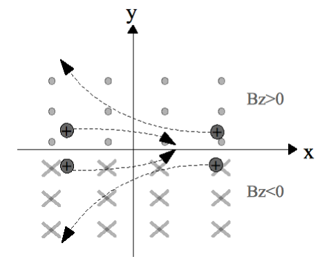
A cartoon of the basic Weibel instability is shown in Fig. 2. Consider a uniform unmagnetized plasma with beams counter-propagating in the x-direction (more generally, possessing an anisotropic temperature with $T_{x}>T_{y},T_{z}$). If a sinusoidal magnetic field component $B_{z}(y)$ arises from noise the positively charged particles with velocities $v_{x}>0$ will converge towards the $x$-axis because of the $\mathbf{V\times B}$ Lorentz force while those with $v_{x}<0$ will diverge. The combination leads to a current density $J_{x}(y)$ of the correct sign to amplify $B_{z}$, thus driving the mode unstable. (Negatively charged particles move in the opposite directions but have the same net effect.)

To explore the structure of the Weibel instability in reconnection generated current layers, we use a fluid description. Since we are considering a pair plasma we include four species, $\alpha\in\{p+,p-,e+,e-$}, in our model: species of positrons and electrons with bulk velocities $\bf{V}$ and $-\bf{V}$. In standard notation the governing equations are:

$$\frac{\partial}{\partial t}n_{\alpha}+\nabla\cdot(n_{\alpha}{\bf V_{\alpha}})=0;$$ (1)

$$m\frac{d}{dt}{\bf V_{\alpha}}=q_{\alpha}{\bf E}+\frac{q_{\alpha}}{c}{\bf V_{\alpha}}\times\ {\bf B}-\frac{\nabla\cdot\mathrm{P}_{\alpha}}{n_{\alpha}};$$ (2)

$$\nabla\times{\bf B}=\frac{4\pi}{c}\sum_{\alpha}n_{\alpha}q_{\alpha}{\bf V_{\alpha}};$$ (3)

$$\frac{\partial}{\partial t}{\bf B}=-c\nabla\times\bf{E}.$$ (4)

We assume the pressure tensor can be written in the diagonal form

$$\mathrm{P}_{\alpha}=n_{\alpha}T_{\alpha}=n_{\alpha}\left[\begin{array}[]{clr}T_{xx,\alpha}&0&0\\ 0&T_{yy,\alpha}&0\\ 0&0&T_{zz,\alpha}\end{array}\right]$$ (5)

and that the temperature components do not vary in space or time.

To particularize our coordinates we take the counter streaming velocities to be parallel to $\mathbf{\hat{x}}$. The perturbed magnetic field of the Weibel mode can then, without loss of generality, be taken to be parallel to $\mathbf{\hat{z}}$ and the wavevector parallel to $\mathbf{\hat{y}}$. All physical quantities are assumed uniform in both the $x$ and $z$ directions, $\partial/\partial_{z}=\partial/\partial_{x}=0$.

Our initial state is characterized by

$$\begin{split}{\bf{V}}=V_{x}(y)\mathbf{\hat{x}};\qquad{\bf{B}}=B_{x}(y)\mathbf{\hat{x}};\\ n_{\alpha}=n(y);\qquad T_{yy,\alpha}=T_{zz,\alpha}=T.\end{split}$$ (6)

Pressure balance requires $\left(4nT_{yy}+B_{x}^{2}/8\pi\right)^{\prime}=0$, where a prime stands for $\partial/\partial y$, and the total number density for either electrons or positrons is $2n$. If all perturbed variables are proportional to $e^{\gamma t}$ we can linearize equations (1)-(4) as

$$\gamma\tilde{n}+n^{\prime}\tilde{V}_{y,\alpha}+n\tilde{V}_{y,\alpha}^{\prime}=0;\\$$ (7)

$$\gamma m\tilde{V}_{x,\alpha}+m\tilde{V}_{y,\alpha}V^{\prime}_{x,\alpha}=q_{\alpha}\tilde{E}_{x};$$ (8)

$$\gamma m\tilde{V}_{y,\alpha}=q_{\alpha}\tilde{E}_{y}+\frac{q_{\alpha}}{c}[\tilde{V}_{z,\alpha}B_{x}-V_{x,\alpha}\tilde{B}_{z}]+T\frac{n^{\prime}}{n^{2}}\tilde{n}-\frac{T}{n}\tilde{n}^{\prime};$$ (9)

$$\gamma m\tilde{V}_{z,\alpha}=q_{\alpha}\tilde{E}_{z}-\frac{q_{\alpha}}{c}\tilde{V}_{y,\alpha}B_{x};$$ (10)

$$\tilde{B}_{z}^{\prime}=\frac{4\pi}{c}\sum_{\alpha}q_{\alpha}(\tilde{n}V_{x,\alpha}+n\tilde{V}_{x,\alpha});$$ (11)

$$\gamma\tilde{B}_{z}=c\tilde{E}_{x}^{\prime},$$ (12)

where a tilde indicates a perturbed quantity.

The effective x-direction temperature is $T_{x}=mV_{x}^{2}+T_{xx}$. Note that by assuming $\partial/\partial x=0$ we eliminate $T_{xx}$ from the equations. The effective temperature anisotropy is then determined only by the streaming velocity.

Due to the mass and charge symmetry between electrons and positrons, we can collapse these eighteen equations, Eq. (7)-Eq. (12), into two second-order differential equations (see Appendix A for details):

$$C_{s}^{2}{\bar{\chi}}^{\prime\prime}-C_{s}^{2}\frac{n^{\prime}}{n}\bar{\chi}^{\prime}-\Omega^{2}\bar{\chi}-\frac{4e}{m}V_{x}n\tilde{E}_{x}^{\prime}=\gamma^{2}\bar{\chi};$$ (13)

$$\tilde{E}_{x}^{\prime\prime}-\frac{2}{d^{2}}\tilde{E_{x}}+\frac{4\pi e}{c^{2}}(V_{x}\bar{\chi})^{\prime}=0$$ (14)

with the following definitions: $\bar{\chi}\equiv n(\tilde{V}_{y,p+}-\tilde{V}_{y,p-}-\tilde{V}_{y,e+}+\tilde{V}_{y,e-})$; $\Omega$ is the gyrofrequency based on $B_{x}$; $C_{s}\equiv\sqrt{T/m}$ is the sound speed; and $d\equiv\sqrt{mc^{2}/8\pi ne^{2}}\equiv c/\omega_{p}$ is the skin depth with $\omega_{p}$ the plasma frequency.

III The Weibel instability in a homogeneous plasma

In a uniform magnetized plasma a dispersion relation can be found by combining Eqs. (13) and (14) and letting $\partial/\partial_{y}\rightarrow ik_{y}$:

$$\gamma^{2}=\frac{2V_{x}^{2}k_{y}^{2}}{2+k_{y}^{2}d^{2}}-C_{s}^{2}k_{y}^{2}-\Omega^{2}.$$ (15)

Clearly while the streaming temperature (the first term of the right hand side) serves as the instability driver, thermal effects in the y-direction (the second term) and the background magnetic field (the third term) stabilize the mode.

In the even simpler case of a strongly anisotropic unmagnetized plasma, the kinetic growth rate of the Weibel instability is Swisdak et al. (2008),Krall and Trivelpiece (1986):

$$\gamma^{2}\approx\frac{2v^{2}_{th,x}k_{y}^{2}}{2+k_{y}^{2}d^{2}},$$ (16)

where $v_{th,x}=\sqrt{T_{x}/m}$ is the thermal velocity in the $x$ direction. It is evident that this matches the first term of Eq. (15) with $v_{th,x}\rightarrow V_{x}$. The validity of using counter streaming cold plasma beams to analyze a single warm plasma was demonstrated by Davidson et al. Davidson et al. (1972), who showed that this instability is not affected by the detailed shape of the plasma distribution function, but only by the effective temperature.

IV The Weibel instability inside a Harris sheet

The results of Section III were derived in the context of a homogeneous plasma. However for reconnection simulations it is important to study how the development of the Weibel instability proceeds inside a narrow current layer. In this section we seek to understand whether, and to what degree, the inhomogeneities in the plasma density and background magnetic field affect the instability.

Our equilibrium is taken to be the usual Harris layer with a slight modification that incorporates an anisotropic plasma temperature

$$B_{x}=B_{x0}\tanh(y/\delta);\qquad n_{p,e}=2n=n_{0}\mbox{sech}^{2}(y/\delta);$$ (17)

$$V_{x}^{2}=(V_{x0}^{2}-C_{s}^{2})\mbox{sech}^{2}(y/\delta)+C_{s}^{2},$$ (18)

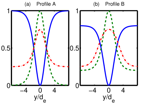
where $B_{x0},n_{0}$, and $V_{x0}$ are constants, $\delta$ measures the width of current sheet and the subscripts p/e stand for positron/electron. We will refer to this setup as Profile A. The profiles are shown in Fig. 3(a).

For the sake of comparing with full particle pair reconnection simulations, all physics quantities are presented in the same normalized units as those in Swisdak et al. Swisdak et al. (2008): the magnetic field to the asymptotic value of the reversed field $B_{x0}$, the density to $n_{0}$ which is the value at the center of the current sheet minus a possible uniform background density, velocities to the electron Alfvén speed $V_{A,e}$, lengths to the electron inertial length $d_{e}\equiv\sqrt{mc^{2}/4\pi n_{0}e^{2}}$, times to the inverse electron cyclotron frequency $\Omega_{ce}^{-1}$, and temperatures to $m_{e}V_{A,e}^{2}$. We use $T=0.25m_{e}V_{A,e}$ in the analysis of this section, which is the initial set up of the pair reconnection simulation of Swisdak et al. (2008), except for the latter’s inclusion of a uniform background density of $0.2n_{0}$.

To find the modes of Eqs. (13) and (14) we discretize the governing equations in the $y$ direction (imposing zero derivative boundary conditions) and find the eigenvalues of the resulting matrix. We use a grid size of $\delta/100$ and domain size of $20\delta$, both of which are sufficient to ensure covergence. Before describing the numerical results, however, we investigate the behavior of the equation analytically.

IV.1 $k_{y}d_{e}\gg 1$, $\delta/d_{e}\ll 1$

In this limit the current layer thickness and the wavelength of the instability are much smaller than the inertial length $d_{e}$. From general considerations we expect the mode to be harder to excite in such circumstances, unless $V_{x}$ is large. It is straightforward to combine Eqs. (13) and (14) into a single second-order ordinary differential equation by eliminating the second term in Eq. (14), which is small since $k_{y}d_{e}\gg 1$. The result is

$$C_{s}^{2}\bar{\chi}^{\prime\prime}-C_{s}^{2}\frac{n^{\prime}}{n}\bar{\chi}^{\prime}+\left(\frac{2V_{x}^{2}}{d^{2}}-\Omega^{2}\right)\bar{\chi}=\gamma^{2}\bar{\chi}.$$ (19)

For the parameter regime of interest, $d/d_{e}\sim\Omega/\Omega_{ce}\sim O(1)$. Therefore for every term in Eq. (19) to be of the same order (except, perhaps, the $\Omega^{2}$ term), the following scaling rules must apply:

$$\gamma\sim V_{x}/d\sim k_{y}C_{s}\gg\Omega\sim C_{s}/d.$$ (20)

After substituting for the functional form of the inhomogeneity and changing variables to $u=\cosh(y/\delta)\bar{\chi}$, we have

$$C_{s}^{2}u^{\prime\prime}=Q(y)u,$$ (21)

where

$$\begin{split}Q=\gamma^{2}-\frac{2}{d_{e}^{2}}\left[V_{x0}^{2}\mbox{sech}^{2}(y/\delta)+C_{s}^{2}\tanh^{2}(y/\delta)\right]\mbox{sech}^{2}(y/\delta)\\ +\Omega_{0}^{2}\tanh^{2}(y/\delta)+\frac{C_{s}^{2}}{\delta^{2}}\end{split}$$ (22)

and $\Omega_{0}\equiv B_{x0}e/mc$. For $V^{2}_{x0}>C_{s}^{2}d_{e}^{2}/2\delta^{2}$, $Q$ is negative near $y=0$ and positive at large $y$ and Eq. (21) therefore has bounded solutions.

We further simplify $Q$ by Taylor expanding for small $y/\delta$, and neglecting the $C_{s}^{2}\tanh^{2}$ and $\Omega_{0}^{2}\tanh^{2}$ terms in Eq. (22), which are small in the ordering given in Eq. (20),

$$C_{s}^{2}u^{\prime\prime}-\frac{2V_{x0}^{2}}{d_{e}^{2}\delta^{2}}y^{2}u=\left(\frac{2V_{x0}^{2}}{d_{e}^{2}}-\frac{C_{s}^{2}}{\delta^{2}}-\gamma^{2}\right)u.$$ (23)

This equation can be solved in terms of Hermite polynomials with eigenvalues that give a maximum growth rate of

$$\gamma_{max}^{2}=\frac{2V_{x0}^{2}}{d_{e}^{2}}-\frac{\sqrt{2}V_{x0}C_{s}}{d_{e}\delta}-\frac{C_{s}^{2}}{\delta^{2}}.$$ (24)

Clearly the density shear term, $C_{s}^{2}/\delta^{2}$, which arises from the second term of Eq. (19), has the strongest stabilizing effect. By letting $\gamma_{max}=0$, we obtain the critical temperature anisotropy required for the unstable mode in the small $\delta/d_{e}$ limit,

$$\left(\frac{T_{x0}}{T}\right)_{c}=\frac{3+\sqrt{5}}{4}\left(\frac{d_{e}}{\delta}\right)^{2},$$ (25)

where $T_{x0}\equiv(T_{x})_{y=0}=mV_{x0}^{2}$.

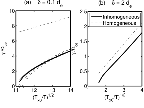
We plot $\gamma$ versus anisotropy in Fig. 4(a) for $\delta=0.1d_{e}$ and in Fig. 4(b) for $\delta=2d_{e}$. In the $\delta=0.1d_{e}$ case, the full equations (Eqs. (13),(14)) and the reduced equation (Eq. (21)) result in the same curve because the wavenumber of the growing mode is large enough to validate the approximation. The analytical solution from Eq. (24) follows the correct trend and matches the numerical results, particularly in the large anisotropy limit. We observe that $\gamma$ is proportional to $V_{x0}$ (i.e., $V_{x0}\sim(T_{x0}/T)^{1/2}$ ) as the scaling rule (Eq. (20)) suggests. By comparing the growth rate of the unmagnetized homogeneous plasma from Eq. (15), it is also clear that the instability is severely suppressed by the inhomogeneity. In contrast, the $\delta=2d_{e}$ case results in a somewhat closer match because of the increase in the inhomogeneity scale length.

IV.2 $k_{y}d_{e}\ll 1$, $\delta/d_{e}\gg 1$

Although in this limit the search for bounded modes is rather complicated, it is possible to gain some insight by expanding the homogeneous dispersion relation, Eq. (15) in the small $k_{y}$ limit:

$$\gamma^{2}\approx V_{x}^{2}k_{y}^{2}\left(1-\frac{d^{2}}{2}k_{y}^{2}\right)-C_{s}^{2}k_{y}^{2}-\Omega^{2}.$$ (26)

If we only keep terms of $O(k_{y}^{2})$ we find that

$$k_{y}^{2}\approx(\gamma^{2}+\Omega^{2})/(V_{x}^{2}-C_{s}^{2}),$$ (27)

which is always positive and has no bounded modes. It is only by keeping the next term (i.e., $O(k_{y}^{4})$) in the expansion that bounded modes exist, a fact that will guide our treatment of the full system.

We begin by neglecting the $\tilde{E}_{x}^{\prime\prime}$ term in Eq. (14), solving for $E_{x}$, and then substituting the result back into the equation, ultimately giving

$$\frac{2}{d^{2}}\tilde{E_{x}}\simeq\frac{4\pi e}{c}(V_{x}\bar{\chi})^{\prime}+\frac{4\pi e}{c}\left(\frac{d^{2}}{2}(V_{x}\bar{\chi})^{\prime}\right)^{\prime\prime}.$$ (28)

We then use this approximation in Eq. (13) in the small $y/\delta$ limit and assume that we are close to marginal stability. The resulting equation is:

$$\frac{V_{x0}^{2}d_{e}^{2}}{2}\bar{\chi}^{\prime\prime\prime\prime}+(V_{x0}^{2}-C_{s}^{2})\bar{\chi}^{\prime\prime}+\frac{\Omega_{0}^{2}}{\delta^{2}}y^{2}\bar{\chi}=-\gamma^{2}\bar{\chi}.$$ (29)

The parameter regime of interest to us is $V_{x0}/V_{A,e}\sim C_{s}/V_{A,e}\sim\Omega_{0}/\Omega_{ce}\sim O(1)$. By requiring each term in this equation to be the same order we arrive at the ordering

$$\gamma^{2}\sim k_{y}^{2}(V^{2}_{x0}-C^{2}_{s});\qquad k_{y}^{2}d_{e}^{2}\sim(V^{2}_{x0}-C^{2}_{s})/V^{2}_{x0}\ll 1.$$ (30)

To proceed, we transform the equation to Fourier space

$$\frac{\Omega_{0}^{2}}{\delta^{2}}\frac{\partial^{2}}{\partial k_{y}^{2}}\bar{\chi}+\left[(V_{x0}^{2}-C_{s}^{2})k_{y}^{2}-\frac{V_{x0}^{2}d_{e}^{2}}{2}k_{y}^{4}\right]\bar{\chi}=\gamma^{2}\bar{\chi}.$$ (31)

The quantity inside the square brackets has a maximum at $k_{y0}=\sqrt{V_{x0}^{2}-C_{s}^{2}}/d_{e}V_{x0}$. Since we are looking for the maximally growing mode, we Taylor expand this quantity in $s\equiv k_{y}-k_{y0}$ around $s=0$:

$$\frac{\Omega_{0}^{2}}{\delta^{2}}\frac{\partial^{2}}{\partial s^{2}}\bar{\chi}-2(V_{x0}^{2}-C_{s}^{2})s^{2}\bar{\chi}=\left[\gamma^{2}-\frac{(V_{x0}^{2}-C_{s}^{2})^{2}}{2d_{e}^{2}V_{x0}^{2}}\right]\bar{\chi}.$$ (32)

The solution of this equation can again be written in the form of Hermite polynomials with a maximal eigenvalue of

$$\gamma_{max}^{2}=\frac{(V_{x0}^{2}-C_{s}^{2})^{2}}{2d_{e}^{2}V_{x0}^{2}}-\frac{\Omega_{0}}{\delta}\sqrt{2(V_{x0}^{2}-C_{s}^{2})}.$$ (33)

Without the second term, which arises from the background magnetic field, the growth rate scales as $\gamma_{max}^{2}\sim(V_{x0}^{2}-C_{s}^{2})k_{y}^{2}$ (with $k_{y}^{2}$ given in Eq. (30)), which is essentially the same result as the unmagnetized homogeneous relation, Eq. (15), in the $k_{y}d_{e}\ll 1$ limit. From Eq. (33), we derive the marginal criterion in the large $\delta/d_{e}$ limit,

$$\left(\frac{T_{x0}}{T}\right)_{c}=1+\left(\frac{2\sqrt{2}\Omega_{0}d_{e}^{2}}{C_{s}\delta}\right)^{2/3}.$$ (34)

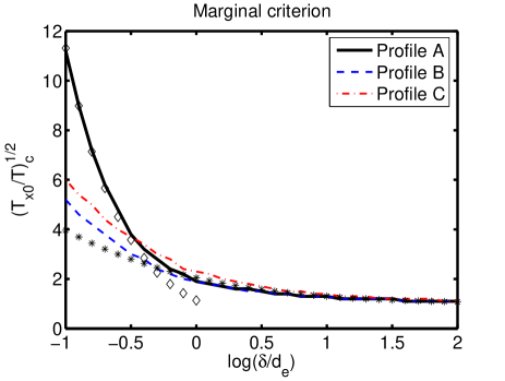
Finally we plot the threshold of marginal instability for different values of $\delta$ in Fig. 5. The numerical solution of our model with Profile A is carefully benchmarked by these asymptotic theories in both the small and large $\delta$ (or $k_{y}$) limits. The (blue) dashed and (red) dot-dashed lines are discussed later.

V The small box PIC simulation

In order to confirm our linear theory and study the nonlinear development of the Weibel instability, we conduct several simulations with the particle-in-cell (PIC) code p3d Zeiler et al. (2002). The electromagnetic fields are defined on gridpoints and advanced in time with an explicit trapezoidal-leapfrog method using second-order spatial derivatives. The Lorentz equation of motion for each particle is evolved by a Boris algorithm where the velocity $\mathbf{v}$ is accelerated by $\mathbf{E}$ for half a timestep, rotated by $\mathbf{B}$, and accelerated by $\mathbf{E}$ for the final half timestep. To ensure that $\bm{\nabla\cdot}\mathbf{E}=4\pi\rho$ a correction electric field is calculated by inverting Poisson’s equation with a multigrid algorithm. Although the code permits other choices, we work with fully periodic boundary conditions.

We consider a system periodic in the $x-y$ plane. The simulations presented here are two-dimensional, i.e., $\partial/\partial z=0$. The initial equilibrium consists of a Harris current sheet superimposed on an ambient population of uniform density $n_{b}$,

$$B_{x}=B_{x,h}\tanh(y/\delta);\qquad n_{p,e}=n_{h}\mbox{sech}^{2}(y/\delta)+n_{b},$$ (35)

where $B_{x,h},n_{h},n_{b}$ are constants, subscript $h$ stands for Harris sheet and $\delta$ is the half width of the current sheet. We input the Harris plasma with an initial temperature $T_{xx,h}>T_{yy}=T_{zz}\equiv T$. The background plasma has an isotropic temperature $T$. Therefore,

$$T_{x}=\frac{n_{b}T+n_{h}\mbox{sech}^{2}(y/\delta)T_{xx,h}}{n_{b}+n_{h}\mbox{sech}^{2}(y/\delta)},$$ (36)

where $T$ and $T_{xx,h}$ are constants. This equilibrium is very similar to Profile A defined in Eqs. (17)-(18) except for the inclusion of a background density. In the following we take the parameters $n_{h}=0.8n_{0},n_{b}=0.2n_{0},B_{x,h}^{2}=0.8B_{x0}^{2},\delta=2d_{e}$ in order to compare later to our full simulations of pair reconnection, and refer to the initial condition as Profile B (see Fig. 3(b)).

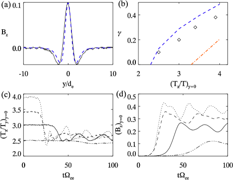
In order to prevent the simultaneous growth of the tearing mode Furth et al. (1963) we consider a domain with $L_{x}=4d_{e}\ll L_{y}=50d_{e}$. We let the Weibel mode grow from noise for different values of the temperature anisotropy, measure the growth rate, and compare the results with the theoretical values from the full four-beam model in Fig. 6(b). Kinetic effects only slightly reduce the growth rates of our four-beam results and the eigenfunction predicted by the model is in good agreement with the simulations (see Fig. 6(a)). The anisotropy threshold for the four-beam model with Profile B is shown as a (blue) dashed line in Fig. 5.

The evolution of the temperature anisotropy and Weibel-generated $B_{z}$ from four small-box runs with different initial conditions is shown in Fig. 6(c)-(d). The anisotropies (at $y=0$) decrease in time to slightly above the marginal value $\sim 2.3$, while the amplitude of $B_{z}$ simultaneously rises. The increase of $B_{z}$ scatters the hot streaming plasma, reducing the central anisotropy. Only a small part of the energy released transfers to $B_{z}$. The scattering increases $T_{yy}$, and therefore the central pressure, causing the layer to expand. As a result, the ambient $B_{x}$ increases due to compression (not shown).

In homogeneous plasmas we can predict the saturation level by analyzing the particle motion in the y-direction, $dV_{y}/dt=-(e/mc)V_{x}B_{z}$. Roughly speaking, the Weibel instability saturates when the magnetic field grows to a value such that the particles become magnetically trapped and can no longer amplify the field. Trapping occurs when the particle excursion along $\hat{y}$, $\Delta y$, is comparable to the wavelength during the mode growth time,

$$\Delta y\sim\frac{eV_{x}B_{z}}{mc\gamma_{max}^{2}}\sim\frac{1}{k_{max}}.$$ (37)

Equivalently,

$$\gamma_{max}\sim\left(\frac{e}{mc}V_{x}B_{z}k_{y,max}\right)^{1/2}=\omega_{B},$$ (38)

The saturation occurs when the magnetic bounce frequency, $\omega_{B}$, is comparable to the fastest linear growth rate. This is essentially the empirical result from Davidson et al.Davidson et al. (1972). In the strong anisotropy limit, $\gamma_{max}\sim V_{x}k_{y,max}$ (Eq. (15)), we obtain the simple saturation criterion $k_{y,max}\rho_{z}\sim 1$, where $\rho_{z}$ is the gyro-radius in the $B_{z}$ field. In our inhomogeneous plasmas the same principle guides the saturation of the Weibel mode, although the predicted saturation value of $B_{z}$ is smaller due to the inhomogeneity.

VI Implications for Pair Reconnection

VI.1 $k_{y}$ structure

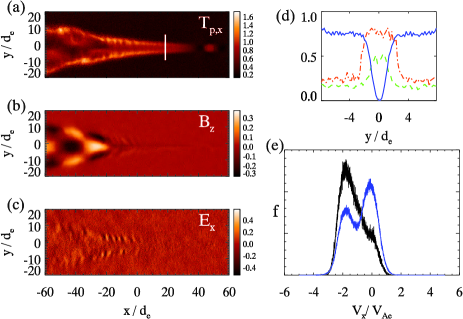
The basic features of a pair plasma reconnection simulation are shown in Fig. 7. The Weibel instability manifests itself as a chess-board-like structure in the downstream out-of-plane magnetic field (see Fig. 7 (b)). The structure travels downstream with the outflow speed from the x-line, which implies that the Weibel is a purely growing mode in the frame of the outflowing plasma. Swisdak et al. Swisdak et al. (2008) proposed that the anisotropy (with typical magnitude $T_{x}/T_{y}\sim 2-4$) driving the instability arises from cold inflowing plasma mixing with outflow from the x-line. Here we apply our analytical results to these observations. After fitting the inhomogeneity (Fig. 7(d)) seen in the reconnection simulations by Eqs. (35)-(36) with parameters $n_{h}=0.25n_{0},n_{b}=0.2n_{0},B_{x,h}^{2}=0.8B_{x0}^{2}$ (denoted Profile C) we can find the necessary temperature anisotropy for Weibel to be unstable within the current layer. The (red) dot-dashed curve in Fig. 5 is the marginal criterion for the Weibel instability, and it gives us the minimum temperature anisotropy $T_{x}/T\sim 3.3$ for a typical reconnection layer of width $4d_{e}$ (i.e., $\delta=2d_{e}$). This predicted minimum is within the observed anisotropy values ($2\sim 4$) and thus demonstrates that the reconnection current layer can support the Weibel mode. The even parity of $B_{z}$ produced by the Weibel mode (Fig. 6(a)) is also seen in the reconnection simulation. Farther downstream, the nonlinear saturation of the Weibel instability stops the system from moving to even higher temperature anisotropies and keeps the system near marginal stability.

The magnitude of $B_{z}$ saturates at $\sim 0.1-0.4B_{x0}$ in Fig. 6(d), which is comparable to the value shown in Fig. 7(b). Therefore by measuring the time, $t_{s}$, for $B_{z}$ to saturate, we can estimate the half-length of the reconnection nozzle as $L\approx V_{A,e}t_{s}$ since $B_{z}$ develops from the instability while the plasma is convected out from the x-point at roughly the electron Alfvén velocity. As a result, anisotropy values of $2.5\sim 4$ with saturation times from Fig. 6(d) give a predicted half-nozzle length in the range $25\sim 80d_{e}$, which compares favorably with the observed reconnection layer half-length of $60d_{e}$. Although these small runs use higher density plasmas than the reconnection runs, we expect the saturation behavior to be similar. Furthermore, the (red) dot-dashed curve in Fig. 6 (b), which represents the four-beam model solution with Profile C, indicates that an anisotropy of $4.0$ produces a growth rate of $\sim 0.2\Omega_{ce}$, which again leads to a nozzle half-length of $\sim 50d_{e}$ (i.e., we expect its evolution to be similar to the solid curve in Fig. 6 (d)).

In contrast to our small-box runs where reconnection was suppressed, we expect the background to be noisier in a simulation that allows both reconnection and the Weibel instability to develop. However that will not strongly affect our results. Since the out-of-plane field $B_{z}$ grows exponentially from the initial noise we expect the estimated nozzle length to scale logarithmically with the initial noise level. Hence the predicted length via this estimate is insensitive to the noise in $B_{z}$ and we can expect our small-box runs to still give a reliable comparison to reconnection simulations.

VI.2 $k_{x}$ structure

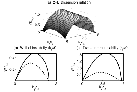
We now focus on the origin and magnitude of the finite $k_{x}$ in the region downstream of the x-line. Loosening our assumptions by letting $\partial/\partial_{x}\neq 0$ in the linearized four-beam model from Eq. (1)-(4), we can numerically solve for the two-dimensional dispersion relation in a homogeneous plasma. One new feature is the introduction of a two-stream instability (i.e., $k_{y}=0$ mode) that has previously been noted by Zenitani & Hesse Zenitani and Hesse (2008) (see Appendix B for the dispersion relation). As shown in Fig. 8, the two-stream instability has a higher growth rate than the Weibel instability. Hence it always grows in front of the Weibel structures with wavelength $\sim 2\pi/3\approx 2d_{e}$, where the factor of 3 comes from the wavenumber for the maximum growth mode measured in Fig. 8(c). We do observe a double peaked distribution of the $x$-direction velocity and the $E_{x}$ signature of the two-stream instability (Fig. 7 (e), (c)) in the appropriate region with a wavelength comparable to the predicted value. The nonlinear development of the two-stream instability tends to merge the counter-streaming distributions, resulting in a single-humped distribution farther downstream with $T_{x}>T_{y}$. The result is a transition from coexisting Weibel and two-stream instabilities to a pure Weibel instability, as can be seen in Fig. 7(b).

The two-stream maximum growth rate predicted by the four-beam model is three times larger than that of the Weibel instability (divide the maximum growth rate of the solid curve in Fig. 8(c) by that of Fig. 8(b)), which seems inconsistent with their relatively close development in the reconnection simulations. However this disagreement can be reduced by the introduction of kinetic effects and a finite $T_{xx}$, both of which are not included in our four-beam model. In particular, a finite $T_{xx}$ suppresses the growth of the two-stream instability. Kinetic theories predict lower growth rates for both the two-stream and Weibel instabilities, with the ratio of their fastest growth rates decreasing to about 1.6 (divide the maximum growth rate of the dashed curve in Fig. 8(c) by that of Fig. 8(b)). This lower ratio helps to explain the nearly coincident signatures of both instabilities in pair reconnection. In general, we also expect that a full kinetic treatment of Harris sheet inhomogeneous plasmas will produce slightly lower Weibel growth rates than those of our four-beam model, a feature that has already been observed in Fig. 6(b).

The two-stream instability can not explain the longer $x$-direction variance of the chess-board-like structure farther downstream. In that region, $B_{x}$ decreases from the asymptotic value of the reversed field ($\approx B_{x0}$) at the nozzle edge to zero at the nozzle symmetry line while the temperature anisotropy remains large. Although Swisdak et al. Swisdak et al. (2008) use a parity argument to argue against the possibility that the firehose instability plays a role, it is perhaps plausible that it could couple to the stronger Weibel mode and provide the finite $k_{x}$. However this possibility is again ruled out by directly solving for the homogeneous dispersion relation of the firehose instability via a one fluid double-adiabatic model with finite Larmor radius corrections Davidson and Volk (1968). The firehose instability in a homogenous plasma with $n_{p,e}=0.45n_{0}$, $T_{x}=4.0T$ has the strongest growth rate $\sim 0.035\Omega_{ce}$ at $B_{x}\sim 0.44B_{x0}$ and $k_{x}d_{e}\sim 0.07$, which is an order of magnitude smaller than the growth rates of the Weibel and two-stream instabilities. Moreover, the predicted wavelength is too large to explain the observed $k_{x}$.

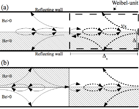
A possible mechanism for the observed $k_{x}$ is proposed here. First imagine that the instability is confined in the $y$ direction between reflecting walls (see Fig. 9). The reflecting walls mimic the strong $B_{x}$ field at the boundaries of the current layer. In this geometry there is an intrinsic scale length $\Delta_{x}$ associated with the trajectory of a particle away from the current layer, its reflection from the wall, and its motion back towards current layer. For a uniform $B_{z}$, $\Delta_{x}=2\sqrt{\rho_{z}^{2}-(\rho_{z}-\Delta)^{2}}$, where $\rho_{z}=V_{x}/\Omega_{c,z}$ is the gyro-radius based on $B_{z}$ and $\Delta$ is the half distance between the walls. The particle trajectory is sketched in the dashed box of Fig. 9(a). We suggest that this intrinsic scale length controls the x-dependence of $B_{z}$ seen in the simulations. We define the scale $\Delta_{x}$ shown as a dashed box in Fig. 9(a) as a Weibel-unit and consider the interaction between two Weibel-units. When all of the converging streaming particles (dashed curves with rightward arrows) leave the center of the righthand Weibel-unit in Fig. 9(a), this unit will need a replenishment of converging streaming particles (solid curves with rightward arrows) from its leftward neighbor to maintain its central current. Hence this self-consistent arrangement can arise without x-variation.

However, suppose that due to the initial random noise the lefthand Weibel-unit acquires the opposite polarity magnetic field, as seen in Fig. 9(b). Then the intrinsic $\Delta_{x}$ will arise such that the source for replenishing the converging streaming particles of the righthand Weibel-unit is the diverging streaming particles (solid curves with rightward arrows) of a leftward neighbor after they bounce (perhaps multiple times) against the walls. The lefthand Weibel-unit can be reinforced from its rightward neighbor in the same manner. In this configuration we can estimate the distance between two neighboring Weibel-units to be $N\Delta_{x}$, where $N$ is the number of times a particle reflects from the walls.

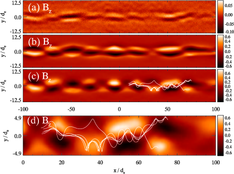
This qualitative explanation is supported by PIC simulations, as can be seen in Fig. 10. We confine an plasma with an anisotropic temperature within a magnetic trough with thickness $5d_{e}$. Specifically, $B_{x}=0$, $T_{x}=4.0T$, and $n=1.2n_{0}$ between $y=-2.5\sim 2.5d_{e}$ and $B_{x}=1.0B_{x0}$, $T_{x}=T$, and $n=0.2n_{0}$ outside this region. The simulation is performed in a domain of size $200d_{e}\times 25d_{e}$ with periodic boundary conditions in both the $x$ and $y$ directions. Here the $B_{x}$ trough serves as the reflecting walls and the trough thickness of $5d_{e}$ is comparable to the reconnection nozzle thickness. Two distant Weibel-units are not able to communicate with each other, and therefore it is not surprising to see that the magnetic fields at $x=-50d_{e}$ and $50d_{e}$ in Fig. 10(a) have opposite signs. As time evolves, the Weibel-generated field gets stronger while the long Weibel-unit ($x=-30d_{e}\sim 30d_{e}$ at Fig. 10(b)) breaks up into smaller Weibel units of opposite polarity at (c). Five test positrons with initial velocity $\sqrt{T_{x}/m}=1.0V_{A,e}$ (i.e., $T_{x}/T=4$) are randomly placed near $(10d_{e},0d_{e})$. Their trajectories are shown as white curves in Fig. 10(c) and are blown up in Fig. 10(d). They are qualitatively similar to those described in Fig. 9(b). The converging motions of those trajectories at the trough center between $x=10\sim 30d_{e}$ and $x=45\sim 65d_{e}$ of Fig. 10(d) contribute to the current for the out-of-plane magnetic field. These particles reflect from $B_{x}$ in between $x=30\sim 45d_{e}$, where they deposit their momenta. At late time, $t\Omega_{ce}=37.5$, the entire channel relaxes to a chain of Weibel units of alternating polarity, whose length scale is approximately determined by $N\Delta_{x}$ with $N\gtrsim 1$.

In order to apply this idea to the downstream regions in reconnection simulations, we approximate the characteristic streaming velocity as $1.0V_{A,e}$ and the averaged out-of-plane magnetic field as $0.2B_{x0}$. This implies a gyro-radius of $5d_{e}$. The layer thickness $\Delta$ is $2d_{e}$ along the reconnection nozzle, and thus $\Delta_{x}$ has a scale of approximately $2\sqrt{5^{2}-(5-2)^{2}}=8d_{e}$, about half of the size of the observed structure in Fig. 7(c). This mechanism roughly explains the scale size of the observed variation. Furthermore, the gyromotion of the reconnection outflow helps explain how the reconnection nozzle broadens downstream. The out-of-plane magnetic field bends the outflow momentum from the $x$ to the $y$-direction. As a result this flow pushes the background Harris magnetic field away from the symmetry line, broadening the current layer.

VII Summary and Discussion

We have developed a four-beam model to study the effects on the Weibel instability of a spatial inhomogeneity arising from a current layer. We have shown that the Weibel instability is able to grow within narrow Harris sheets, and its growth rate (saturation time), saturation magnitude, and mode structure fit those values observed in pair reconnection.

This further suggests that the Weibel instability might control the current layer dynamics in pair reconnection, where the Hall term is absent. Other candidate instabilities, such as the two-stream and firehose instabilities have rather minor effects, particularly since it is not clear if the firehose instability even appears in these systems. The high-velocity outflow scatters into the transverse direction due to the Lorentz force arising from the Weibel-generated out-of-plane magnetic field. We argue that the associated increased pressure $P_{yy}$ is responsible for opening the pair reconnection nozzle and shortening the current layer. As a consequence, the shorter current layer generates a higher reconnection rate.

Even though a similar temperature anisotropy also could arise in electron-proton reconnection, signatures of the Weibel instability are not seen there. The reason is that the even shorter current layer ($\sim 10d_{e}$), controlled by whistler waves Mandt et al. (1994), leaves insufficient space for the unstable Weibel mode to grow. It is an open question as to how the Weibel instability controlled reconnection transforms into whistler mediated reconnection as the electron to ion mass ratio changes.

The development of the Weibel instability in the initial state of relativistic ($k_{B}T\sim mc^{2}$) pair reconnection is described in Zenitani & Hesse Zenitani and Hesse (2008). There the Weibel instability is shown to grow in front of a tangential discontinuity formed by the mixing of outflowing and ambient plasma, but it is not clear if this turbulence plays a role in the steady-state development of the outflow exhaust and the associated current layer. However, by artificially suppressing the Weibel-generated out-of-plane magnetic field, they do demonstrate the ability of the Weibel mode to broaden the current layer, similar to the behavior of the present non-relativistic case. The growth rate and wave vector of the relativistic Weibel instability are smaller by a factor of $\gamma_{L}^{1/2}$, where $\gamma_{L}$ is the Lorentz factor Yoon and Davidson (1987). Consequently, we expect the instability to grow more slowly during relativistic pair reconnection, not only because of the intrinsically lower growth rate but also because of the relatively larger suppressing effect of the Harris reversed field on the enlarged mode structure (if we assume a similar nozzle thickness in both the relativistic and non-relativistic regimes). Overall, it remains an open question as to whether the Weibel instability plays an important role in controlling relativistic electron-positron reconnection.

Figure 1: (Color online) Out-of-plane electron velocity for two pair reconnection simulations. In (a) the current layer length is about $\sim 120d_{e}$ (i.e., $|x|\lesssim 60d_{e}$) Swisdak et al. (2008). In (b) the current layer length of a simulation with $B_{z}=0$ scales as the system size, $\sim 700d_{e}$ (i.e., $|x|\lesssim 350d_{e}$). The structure in the large island, which may be due to a two-stream instability, does not affect the behavior near the x-line.

Figure 2: Schematic of the Weibel instability.

Figure 3: (Color online) Current sheet profiles. (Blue) solid curves are $B_{x}^{2}$, (green) dashed curves are the positron/electron density $n_{p,e}$, and (red) dot-dashed curves are x-direction temperature $T_{x}$. Profile A in (a) with $n_{0}=1.0n_{0}$, $B_{x0}=1.0B_{x0}$, and $\delta=2d_{e}$. Profile B in (b) with $n_{h}=0.8n_{0},n_{b}=0.2n_{0},B_{x,h}^{2}=0.8B_{x0}^{2}$ and $\delta=2d_{e}$.

Figure 4: Maximum growth rate versus temperature anisotropy for Profile A for (a) $\delta=0.1d_{e}$ and (b) $\delta=2d_{e}$. Thick solid curves: numerical solutions of the full four-beam model, Eqs. (13)-(14). Thin solid curve (only in (a)): numerical solutions of the reduced equation, Eq. (19). Diamonds (only in (a)): analytical solutions in the large-k limit, Eq. (24). Dashed curves: analytical solutions for an unmagnetized homogenous plasma, Eq. (15).

Figure 5: (Color online) The marginal threshold of the Weibel instability as a function of $\delta$. Profile A: the solid curve from the numerical solutions of the full four-beam model (Eqs. (13)-(14)), the diamonds from the analytical solution in the small-$\delta$ limit (Eq. (25)), and stars from the analytical solution in the large-$\delta$ limit (Eq. (34)). Profile B: the (blue) dashed curve from numerical solutions of the full four-beam model. Profile C: the (red) dot-dashed curve from numerical solutions of the full four-beam model.

Figure 6: (Color online) Results from PIC simulations with initial Profile B. In (a) the eigenfunction of $B_{z}$ with $T_{x0}/T=3.0$: in solid the small-box PIC simulation and in (blue) dash the full four-beam model. In (b) the maximum growth rate versus anisotropy: in diamond the small-box PIC simulations, in (blue) dash the full four-beam model and in (red) dot-dash the full four-beam model with Profile C. In (c) the temporal evolution of different initial temperature anisotropies in the small-box PIC simulation. In (d) the magnitude of $B_{z}$ (at $y=0$) for the temperature anisotropies plotted in (c).

Figure 7: (Color online) A PIC simulation of pair reconnection. In (a) the x-direction positron temperature. The X-point is on the right edge of the plot. In (b) the $B_{z}$ signatures of both the Weibel (chess-board-like structure) and two-stream (finer structure upstream) instabilities. In (c) the $E_{x}$ signature of the two-stream instability in the downstream region. In (d) the inhomogeneity plotted along the white line in (a). The line styles (colors) are the same as in Fig. 3. In (e) the double-humped velocity distribution function (blue) in the two-stream and Weibel unstable region ($x/d_{e},y/d_{e}\in(-21:18,-4:4)$) becomes single-humped (black) farther downstream ($x/d_{e},y/d_{e}\in(-44:-30,-4:4)$).

Figure 8: Homogeneous plasma dispersion relation with $c=5V_{A,e},n_{p,e}=0.45n_{0},B_{x}=0,T_{x}=4T_{yy}=4.0m_{e}V_{A,e}^{2}$. In (a) the growth rate as a function of $k_{x}$ and $k_{y}$. In (b) the homogeneous dispersion relation for the Weibel instability. The solid curve corresponds to the four-beam model and the dashes to kinetic theory. In (c) the homogeneous dispersion relation of the two-stream instability. The solid curve corresponds to a the four-beam model with $T_{xx}=0$. The dashed curve is kinetic theory with $T_{xx}=T_{yy}=0.25m_{e}V_{A,e}^{2}$.

Figure 9: Schematic explanation of the interaction between Weibel-units. White regions have $B_{z}>0$, hatched $B_{z}<0$. A Weibel-unit is represented by particle trajectories similar to the dashed curves of Fig. 2. In (a) the converging particles of the right Weibel-unit are replenished by the converging particles from the left unit. In (b) converging particles of the right Weibel-unit can be replenished by diverging particles from the left unit of opposite polarity.

Figure 10: (Color online) Evolution of the Weibel instability with initial anisotropy $4.0$ inside a magnetic field trough. In (a)–(c), $B_{z}$ at $t\Omega_{ce}=12.5,25,37.5$. White curves mark the trajectories of five test positrons with initial velocity $\sqrt{T_{x}/m}=1.0V_{A,e}$ and initial position ($10d_{e},0d_{e}$). In (d) enlargement of the particle trajectories at time $37.5/\Omega_{ce}$.

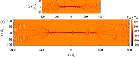
VIII Appendix A: The derivation of the governing equations (13) and (14)

To derive Eqs. (13) and (14), we define the variables,

$$\tilde{\zeta}\equiv\tilde{V}_{x,p+}+\tilde{V}_{x,p-}-\tilde{V}_{x,e+}-\tilde{V}_{x,e-},$$ (39)

$$\tilde{\chi}\equiv\tilde{V}_{y,p+}-\tilde{V}_{y,p-}-\tilde{V}_{y,e+}+\tilde{V}_{y,e-},$$ (40)

$$\tilde{\vartheta}\equiv\tilde{V}_{z,p+}-\tilde{V}_{z,p-}+\tilde{V}_{z,e+}-\tilde{V}_{z,e-},$$ (41)

$$\tilde{\eta}\equiv\tilde{n}_{p+}-\tilde{n}_{p-}-\tilde{n}_{e+}+\tilde{n}_{e-},$$ (42)

then combine Eqs. (7)-(12) to yield

$$-\gamma\tilde{\eta}=n^{\prime}\tilde{\chi}+n\tilde{\chi}^{\prime},$$ (43)

$$\gamma m\tilde{\zeta}=4e\tilde{E_{x}}-mV_{x}^{\prime}\tilde{\chi},$$ (44)

$$\gamma m\tilde{\chi}=\frac{e}{c}B_{x}\tilde{\vartheta}-\frac{4e}{c}V_{x}\tilde{B_{z}}+T\frac{n^{\prime}}{n^{2}}\tilde{\eta}-\frac{T}{n}\tilde{\eta}^{\prime},$$ (45)

$$\gamma m\tilde{\vartheta}=-\frac{e}{c}B_{x}\tilde{\chi},$$ (46)

$$\tilde{B_{z}}^{\prime}=\frac{4\pi e}{c}V_{x}\tilde{\eta}+\frac{4\pi e}{c}n\tilde{\zeta},$$ (47)

$$\gamma\tilde{B_{z}}=c\tilde{E_{x}}^{\prime}.$$ (48)

Eqs. (43)-(48) represent a set of $6$ equations for the $6$ variables, $\{\tilde{\eta},\tilde{\zeta},\tilde{\chi},\tilde{\vartheta},\tilde{B_{z}},\tilde{E_{x}}\}$. Note that $\{n,V_{x},B_{x},T\}$ are unperturbed quantities specifying the initial conditions. Now use Eqs. (43), (44), and (48) to rewrite Eq. (45) in terms of $\tilde{\chi}$ and $\tilde{E_{x}}$,

$$\gamma^{2}\tilde{\chi}=-\Omega^{2}\tilde{\chi}-\frac{4e}{m}V_{x}\tilde{E_{x}}^{\prime}+C_{s}^{2}\left(\frac{(n\tilde{\chi})^{\prime}}{n}\right)^{\prime}.$$ (49)

Use Eqs. (43), (46), and (48) to rewrite Eq. (47) in terms of $\tilde{\chi}$ and $\tilde{E_{x}}$,

$$\tilde{E_{x}}^{\prime\prime}=-\frac{4\pi e}{c^{2}}V_{x}(n\tilde{\chi})^{\prime}+\frac{2}{d^{2}}\tilde{E_{x}}-\frac{4\pi e}{c^{2}}V_{x}^{\prime}n\tilde{\chi}.$$ (50)

After some minor algebraic manipulations, Eqs. (49) and (50) can be written in the form shown in Eq. (13) and (14).

IX Appendix B: The dispersion relations of the two-stream instability and the Weibel instability

If we consider the $k_{y}=0,k_{x}\neq 0$ limit of our four-beam model, we arrive at the usual two-stream instability dispersion relation,

$$1=\frac{\omega_{p}^{2}}{(k_{x}V_{x}-\omega)^{2}}+\frac{\omega_{p}^{2}}{(k_{x}V_{x}+\omega)^{2}},$$ (51)

where $\omega=\omega_{r}+i\gamma$.

The kinetic version of this dispersion relation with finite $T_{xx}$ is

$$\ k_{x}^{2}C_{s}^{2}+\omega_{p}^{2}[2+\xi_{1}Z(\xi_{1})+\xi_{2}Z(\xi_{2})]=0,$$ (52)

where $Z(\xi)\equiv(1/\sqrt{\pi})\int_{-\infty}^{\infty}\mbox{exp}(-x^{2})/(x-\xi)dx$, $\xi_{1}\equiv(\omega/|k_{x}|-V_{x})/\sqrt{2T_{xx}/m}$ and $\xi_{2}\equiv(\omega/|k_{x}|+V_{x})/\sqrt{2T_{xx}/m}$.

For reference, the dispersion relation for the Weibel instability ($k_{x}=0,k_{y}\neq 0$) in kinetic theory is

$$k_{y}^{2}c^{2}-\omega^{2}+2\omega_{p}^{2}\left(1-\frac{T_{x}}{T_{y}}\right)=2\omega_{p}^{2}\frac{T_{x}}{T_{y}}\xi Z(\xi),$$ (53)

where $\xi\equiv\omega/(|k_{y}|\sqrt{2T_{y}/m})$. Note that this reduces to Eq. (16) in the strong anisotropy limit.

If both $k_{x}$ and $k_{y}\neq 0$, both instabilities are present. We treat this limit numerically because of the complexity.

References

- Weibel (1959) E. S. Weibel, Phys. Rev. Lett. 2, 83 (1959).
- Medvedev and Loeb (1999) M. V. Medvedev and A. Loeb, Astrophys. J. 526, 697 (1999).
- Gruzinov and Waxman (1999) A. Gruzinov and E. Waxman, Astrophys. J. 511, 852 (1999).
- Chang et al. (2008) P. Chang, A. Spitkovsky, and J. Arons, Astrophys. J. 674, 378 (2008).
- Spitkovsky (2008) A. Spitkovsky, Astrophys. J. 682, L5 (2008).
- Birn et al. (2001) J. Birn, J. F. Drake, M. A. Shay, B. N. Rogers, R. E. Dention, M. Hesse, M. Kuznetsova, Z. W. Ma, A. Bhattacharjee, A. Otto, J. Geophys. Res. 106, 3715 (2001).
- Bessho and Bhattacharjee (2005) N. Bessho and A. Bhattacharjee, Phys. Rev. Lett. 95, 245001 (2005).
- Daughton and Karimabadi (2007) W. Daughton and H. Karimabadi, Phys. Plasmas 14, 072303 (2007).
- Swisdak et al. (2008) M. Swisdak, Y.-H. Liu, and J. F. Drake, Astrophys. J. 680, 999 (2008).
- Petschek (1964) H. E. Petschek, in Proc. AAS-NASA Symp. Phys. Solar Flares (1964), vol. 50 of NASA-SP, pp. 425–439.
- Krall and Trivelpiece (1986) N. A. Krall and A. W. Trivelpiece, Principles of Plasma Physics (San Francisco Press, Inc., 1986), chap. 9, pp. 483–494.
- Davidson et al. (1972) R. C. Davidson, D. A. Hammer, I. Haber, and C. E. Wagner, Physics of Fluids 15, 317 (1972).
- Zeiler et al. (2002) A. Zeiler, D. Biskamp, J. F. Drake, B. N. Rogers, M. A. Shay, and M. Scholer, J. Geophys. Res. 107, 1230 (2002).
- Furth et al. (1963) H. Furth, J. Killeen, and M. N. Rosenbluth, Physics of Fluids 6, 459 (1963).
- Zenitani and Hesse (2008) S. Zenitani and M. Hesse, Phys. Plasmas 15, 022101 (2008).
- Davidson and Volk (1968) R. C. Davidson and H. J. Volk, Physics of Fluids 11, 2259 (1968).
- Mandt et al. (1994) M. E. Mandt, R. E. Denton, and J. F. Drake, Geophys. Res. Lett. 21, 73 (1994).
- Yoon and Davidson (1987) P. H. Yoon and R. C. Davidson, Phys. Rev. Lett. A 35, 2718 (1987).