Entanglement witnesses and geometry of entanglement of two–qutrit states

Abstract

We construct entanglement witnesses with regard to the geometric structure of the Hilbert–Schmidt space and investigate the geometry of entanglement. In particular, for a two–parameter family of two–qutrit states that are part of the magic simplex we calculate the Hilbert–Schmidt measure of entanglement. We present a method to detect bound entanglement which is illustrated for a three–parameter family of states. In this way, we discover new regions of bound entangled states. Furthermore, we outline how to use our method to distinguish entangled from separable states.

I Introduction

Entanglement is one of the most striking features of quantum theory and is of capital importance for the whole field of quantum information theory (see, e.g., Refs. Bertlmann and Zeilinger (2002); Bouwmeester et al. (2000); Nielsen and Chuang (2000)). The determination whether a given quantum state is entangled or separable is still an open and challenging problem, in particular for higher dimensional systems.

For a two–qubit system the geometric structure of the entangled and separable states in the Hilbert–Schmidt space is very well known. Due to the Peres–Horodecki criterion Peres (1996); Horodecki et al. (1996) we know necessary and sufficient conditions for separability. This case is, however, due to its high symmetry quite unique and even misleading for conclusions in higher dimensions.

In higher dimensions, the geometric structure of the states is much more complicated and new phenomena like bound entanglement occur Horodecki et al. (2001); Horodecki (1997); Horodecki et al. (1998, 1999); Rains (1999); Baumgartner et al. (2007). Although we do not know necessary and sufficient conditions à la Peres–Horodecki we can construct an operator – entanglement witness – which provides via an inequality a criterion for the entanglement of the state Terhal (2000, 2002); Horodecki et al. (1996); Bertlmann et al. (2002).

In this paper, we use entanglement witnesses to explore the geometric structure of the two–qutrit states in Hilbert–Schmidt space, i.e. we geometrically quantify entanglement for special cases, and present a method to detect bound entanglement. Two qutrits are states on the $3\times 3$ dimensional Hilbert space of bipartite quantum systems. In analogy to the familiar two–qubit case, which we discuss at the beginning, we introduce a two– and three–parameter family of two–qutrit states which are part of the magic simplex of states Baumgartner et al. (2006, 2007, 2008) and determine geometrical properties of the states: For the two–parameter family we quantify the entanglement via the Hilbert–Schmidt measure, for the three–parameter family we discover bound entangled states in addition to known ones in the simplex Horodecki et al. (1999); Baumgartner et al. (2006). Finally, we give a sketch of how to use our method to construct the shape of the separable states for the three–parameter family.

II Weyl operator basis

As standard matrix basis we consider the standard matrices, the $d\times d$ matrices, that have only one entry $1$ and the other entries $0$ and form an orthonormal basis of the Hilbert–Schmidt space, which is the space of operators that act on the states of the Hilbert space ${\cal H}^{d}$ of dimension $d$. We write these matrices shortly as operators

$$|j\rangle\langle k|\,,\qquad\textrm{with}\quad j,k=1,\ldots,d\,,$$ (1)

where the matrix representation can be easily obtained in the standard vector basis $\left\{|i\rangle\right\}$. Any matrix can easily be decomposed into a linear combination of matrices (1).

The Weyl operator basis (WOB) of the Hilbert–Schmidt space of dimension $d$ consists of the following $d^{2}$ operators (see Ref. Bertlmann and Krammer (2008a))

$$U_{nm}\;=\;\sum_{k=0}^{d-1}e^{\frac{2\pi i}{d}\,kn}\,|k\rangle\langle(k+m)\,\textrm{mod}\,d|\qquad n,m=0,1,\ldots,d-1\,.$$ (2)

These operators have been frequently used in the literature (see e.g. Refs. Narnhofer (2006); Baumgartner et al. (2006, 2007); Bennett et al. (1993)), in particular, to create a basis of $d^{2}$ maximally entangled qudit states Narnhofer (2006); Werner (2001); Vollbrecht and Werner (2000).

Example. In the case of qutrits, i.e. of a three–dimensional Hilbert space, the Weyl operators (2) have the following matrix form:

$$U_{00} =\begin{pmatrix}1&0&0\\ 0&1&0\\ 0&0&1\end{pmatrix},\quad\qquad\qquad\,U_{01}=\begin{pmatrix}0&1&0\\ 0&0&1\\ 1&0&0\end{pmatrix},\quad\qquad\qquad\,U_{02}=\begin{pmatrix}0&0&1\\ 1&0&0\\ 0&1&0\end{pmatrix},$$

$$U_{10} =\begin{pmatrix}1&0&0\\ 0&e^{2\pi i/3}&0\\ 0&0&e^{-2\pi i/3}\end{pmatrix},\quad U_{11}=\begin{pmatrix}0&1&0\\ 0&0&e^{2\pi i/3}\\ e^{-2\pi i/3}&0&0\end{pmatrix},\quad U_{12}=\begin{pmatrix}0&0&1\\ e^{2\pi i/3}&0&0\\ 0&e^{-2\pi i/3}&0\end{pmatrix},$$

$$U_{20} =\begin{pmatrix}1&0&0\\ 0&e^{-2\pi i/3}&0\\ 0&0&e^{2\pi i/3}\end{pmatrix},\quad U_{21}=\begin{pmatrix}0&1&0\\ 0&0&e^{-2\pi i/3}\\ e^{2\pi i/3}&0&0\end{pmatrix},\quad U_{22}=\begin{pmatrix}0&0&1\\ e^{-2\pi i/3}&0&0\\ 0&e^{2\pi i/3}&0\end{pmatrix}.$$

Using the WOB we can decompose quite generally any density matrix in form of a vector, called Bloch vector Bertlmann and Krammer (2008a)

$$\rho\;=\;\frac{1}{d}\,\mathbbm{1}\,+\,\sum_{n,m=0}^{d-1}b_{nm}U_{nm}\;=\;\frac{1}{d}\,\mathbbm{1}\,+\,\vec{b}\cdot\vec{U}\,,$$ (4)

with $n,m=0,1,...,d-1$ ($b_{00}=0$). The components of the Bloch vector $\vec{b}=\big{(}\{b_{nm}\}\big{)}$ are ordered and given by $b_{nm}=\textnormal{Tr}\,U_{nm}\,\rho\,$. In general, the components $b_{nm}$ are complex since the Weyl operators are not Hermitian and the complex conjugates fulfil the relation $b_{n\,m}^{\ast}=e^{-\frac{2\pi i}{d}\,nm}\,b_{{-n}{-m}}\,$, which follows easily from definition (2) together with the hermiticity of $\rho\,$. Note that for $d\geq 3$ not any vector $\vec{b}$ of complex components is a Bloch vector, i.e. a quantum state (details can be found in Ref. Bertlmann and Krammer (2008a)).

The standard matrices (1), on the other hand, can be expressed by the WOB as Bertlmann and Krammer (2008a)

$$|j\rangle\langle k|\;=\;\frac{1}{d}\,\sum_{l=0}^{d-1}e^{-\frac{2\pi i}{d}\,lj}\;U_{l\,(k-j)\,\textrm{mod}\,d}\;.$$ (5)

It allows us to decompose any two–qudit state of a bipartite system in the $d\times d$ dimensional Hilbert space ${\cal H}^{\,d}_{A}\otimes{\cal H}^{\,d}_{B}$ into the WOB. In particular, we consider the isotropic two–qudit state $\rho_{\alpha}^{(d)}$ which is defined as follows Horodecki and Horodecki (1999); Rains (1999); Horodecki et al. (2001)  :

$$\rho_{\alpha}^{(d)}\;=\;\alpha\left|\phi_{+}^{d}\right\rangle\left\langle\phi_{+}^{d}\right|\,+\,\frac{1-\alpha}{d^{2}}\,\mathbbm{1}\,,\quad\alpha\in\mathbbm{R}\,,\quad-\frac{1}{d^{2}-1}\leq\alpha\leq 1\;.$$ (6)

The range of $\alpha$ is determined by the positivity of the state.

The state

$$\left|\phi^{d}_{+}\right\rangle\;=\;\frac{1}{\sqrt{d}}\,\sum_{j}\left|j\right\rangle\otimes\left|j\right\rangle$$ (7)

denotes a Bell state, which is maximally entangled, and in terms of the WOB it is expressed by (see Refs. Bertlmann and Krammer (2008a); Narnhofer (2006))

$$\left|\phi_{+}^{d}\right\rangle\left\langle\phi_{+}^{d}\right|\;=\;\frac{1}{d^{2}}\,\mathbbm{1}\otimes\mathbbm{1}\,+\,\frac{1}{d^{2}}\,U\,,$$ (8)

with

$$U\;:=\;\sum_{l,m=0}^{d-1}U_{lm}\otimes U_{-lm}\,,\qquad(l,m)\neq(0,0)\,.$$ (9)

The negative values of the index $l$ have to be considered as $mod\ d\,$.

Then the isotropic two–qudit state follows from Eq. (8):

$$\rho^{(d)}_{\alpha}\;=\;\frac{1}{d^{2}}\,\mathbbm{1}\otimes\mathbbm{1}\,+\,\frac{\alpha}{d^{2}}\,U\,.$$ (10)

We call decomposition (10) Bloch vector form of the density matrix.

III Entanglement witness — Hilbert–Schmidt measure

III.1 Definitions

The Hilbert–Schmidt (HS) measure of entanglement Witte and Trucks (1999); Ozawa (2000); Bertlmann et al. (2002) is defined as the minimal HS distance of an entangled state $\rho_{\rm{ent}}$ to the set of separable states $S$,

$$D(\rho_{\rm{ent}})\;:=\;\min_{\rho\in S}\left\|\rho-\rho_{\rm{ent}}\right\|\;=\;\left\|\rho_{0}-\rho_{\rm{ent}}\right\|\,,$$ (11)

where $\rho_{0}$ denotes the nearest separable state, the minimum of the HS distance.

An entanglement witness $A$ is a Hermitian operator that “detects” the entanglement of a state $\rho_{\rm ent}$ via inequalities Horodecki et al. (1996); Terhal (2000, 2002); Bertlmann et al. (2002); Bertlmann and Krammer (2008a)

$$\left\langle\rho_{\rm ent},A\right\rangle\;=\;\textnormal{Tr}\,\rho_{\rm ent}A \;<\; 0\,,$$

$$\left\langle\rho,A\right\rangle=\textnormal{Tr}\,\rho A \;\geq\; 0\qquad\forall\rho\in S\,.$$ (12)

An entanglement witness is “optimal”, denoted by $A_{\rm{opt}}\,$, if apart from Eq. (III.1) there exists a separable state $\rho_{0}\in S$ such that

$$\left\langle\rho_{0},A_{\rm{opt}}\right\rangle\;=\;0\,.$$ (13)

The operator $A_{\rm{opt}}$ defines a tangent plane to the set of separable states $S$ and can be constructed in the following way Bertlmann et al. (2002, 2005) :

$$A_{\rm{opt}}\;=\;\frac{\rho_{0}-\rho_{\rm ent}\,-\,\left\langle\rho_{0},\rho_{0}-\rho_{\rm ent}\right\rangle\mathbbm{1}}{\left\|\rho_{0}-\rho_{\rm ent}\right\|}\;.$$ (14)

The term $\left\|\rho_{0}-\rho_{\rm ent}\right\|$ is a normalization factor and is included for a convenient scaling of the inequalities (III.1) only. Thus, the calculation of the optimal entanglement witness $A_{\rm{opt}}$ to a given entangled state $\rho_{\rm ent}$ reduces to the determination of the nearest separable state $\rho_{0}\,$. In special cases, we are able to find $\rho_{0}$ by a guess method Bertlmann et al. (2005), what we demonstrate in this article by working with our Lemmas, but in general its detection is quite a difficult task.

III.2 Two–parameter entangled states — qubits

It is quite illustrative to start with the familiar case of a two–qubit system to gain some intuition of the geometry of the states in the HS space. We aim to determine the entanglement witness and the HS measure of entanglement for the following two–qubit states which are a particular mixture of the Bell states $|\psi^{-}\rangle,|\psi^{+}\rangle,|\phi^{-}\rangle,|\phi^{+}\rangle$:

$$\rho_{\alpha,\beta}\;=\;\frac{1-\alpha-\beta}{4}\,\mathbbm{1}\,+\,\alpha|\phi^{+}\rangle\langle\phi^{+}|\,+\,\frac{\beta}{2}\left(|\psi^{+}\rangle\langle\psi^{+}|\,+\,|\psi^{-}\rangle\langle\psi^{-}|\right)\,.$$ (15)

The states (15) are characterized by the two parameters $\alpha$ and $\beta$ and we will refer to the states as the two–parameter states. Of course, the positivity requirement $\rho_{\alpha,\beta}\geq 0$ constrains the possible values of $\alpha$ and $\beta$, namely

$$\alpha\;\leq\;-\beta+1,\quad\;\alpha\;\geq\;\frac{1}{3}\beta-\frac{1}{3},\quad\;\alpha\;\leq\;\beta+1\,,$$ (16)

which geometrically corresponds to a triangle, see Fig. 1.

According to Peres Peres (1996) and the Horodeckis Horodecki et al. (1996) the separability of the states is determined by the positive partial transposition criterion, which says that a separable state has to stay positive under partial transposition (PPT). For dimensions $2\times 2$ and $2\times 3$ the criterion is necessary and sufficient Horodecki et al. (1996), thus any PPT state is separable for these dimensions. States (15) which are positive under partial transposition have the following constraints:

$$\alpha\;\geq\;\beta-1,\quad\;\alpha\;\leq\;\frac{1}{3}\beta+\frac{1}{3},\quad\;\alpha\geq-\beta-1\,,$$ (17)

and correspond to the rotated triangle; then the overlap, a rhombus, represents the separable states, see Fig. 1.

In the illustration of Fig. 1 the orthogonal lines are indeed orthogonal in HS space. Therefore, the coordinate axes for the parameter $\alpha$ and $\beta$ are necessarily non–orthogonal. In particular, the $\alpha$ axis has to be orthogonal to the boundary line $\alpha=1/3(\beta-1)$, and the $\beta$ axis has to be orthogonal to $\alpha=\beta+1$.

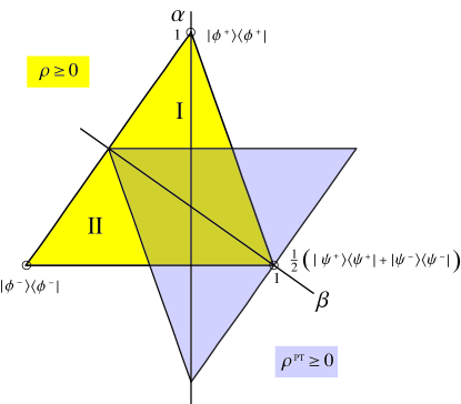
Figure 1: Illustration of the two–qubit states $\rho_{\alpha,\beta}$ (15) and their partial transpositions $\rho^{\rm{PT}}$.

The two–parameter states $\rho_{\alpha,\beta}$ define a plane in the HS space. It is quite illustrative to see how this plane is located in the three–dimensional simplex formed by states that are mixtures of the the four two-qubit Bell states. The simplex represents a tetrahedron due to the positivity conditions of the density matrix Bertlmann et al. (2002); Vollbrecht and Werner (2001); Horodecki and Horodecki (1996). Applying PPT, the tetrahedron is rotated producing an intersection – a double pyramid – which corresponds to the separable states. An illustration of the described features is given in Fig. 2.

To calculate the HS measure (11) for the two–parameter qubit state (15) we express the state in terms of the Pauli matrix basis

$$\rho_{\alpha,\beta}\;=\;\frac{1}{4}\left(\mathbbm{1}\,+\,\alpha\left(\sigma_{1}\otimes\sigma_{1}\,-\,\sigma_{2}\otimes\sigma_{2}\right)\,+\,\left(\alpha-\beta\right)\sigma_{3}\otimes\sigma_{3}\right)\,,$$ (18)

where we have used the well–known Pauli matrix decomposition of the Bell states (see, e.g., Ref. Bertlmann et al. (2002)).

In order to determine the HS measure for the entangled two–parameter states $\rho_{\alpha,\beta}^{\rm{ent}}$ we have to find the nearest separable states, which is usually the most difficult task to perform in this context. In Ref. Bertlmann et al. (2005) a Lemma is presented to check if a particular separable state is indeed the nearest separable state to a given entangled one.

Lemma 1.

A state $\tilde{\rho}$ is equal to the nearest separable state $\rho_{0}$ if and only if the operator

$$\tilde{C}\;=\;\frac{\tilde{\rho}-\rho_{\rm ent}\,-\,\left\langle\tilde{\rho},\tilde{\rho}-\rho_{\rm ent}\right\rangle\mathbbm{1}}{\left\|\tilde{\rho}-\rho_{\rm ent}\right\|}$$ (19)

is an entanglement witness.

Lemma 1 probes if a guess $\tilde{\rho}$ is indeed correct for the nearest separable state. If this is the case, operator $\tilde{C}$ represents the optimal entanglement witness $A_{\rm{opt}}$ (14).

Lemma 1 is used here in the following way. First, for any entangled two-parameter state (15) we calculate the separable state that has the nearest Euclidean distance in the geometric picture (Fig. 1) and call this state $\tilde{\rho}$. But since the regarded picture does not represent the full state space (e.g., states containing terms like $a_{i}\,\sigma^{i}\otimes\mathbbm{1}$ or $b_{i}\,\mathbbm{1}\otimes\sigma^{i}$ are not contained on the picture), we have to use Lemma 1 to check if the estimated state $\tilde{\rho}$ is indeed the nearest separable state $\rho_{0}$.

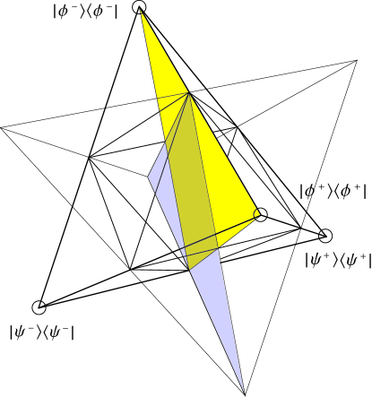
Figure 2: Location of the plane of states $\rho_{\alpha,\beta}$ (15) in the tetrahedron formed by the Bell states.

III.2.1 Region I

Let us consider first the entangled states located in the triangle region that includes the Bell state $|\phi^{+}\rangle\,$, i.e. Region I in Fig. 1. An entangled state in Region I is characterized by points, i.e. by the parameter pair ($\alpha$,$\beta$), constrained by

$$\alpha\;\leq\;\beta+1,\quad\;\alpha\;\leq\;-\beta+1,\quad\;\alpha\;>\;\frac{1}{3}\beta+\frac{1}{3}\,.$$ (20)

The point in the separable region of Fig. 1 that is nearest (in the Euclidean sense) to the point ($\alpha$,$\beta$) is given by ($\frac{1}{3}+\frac{1}{3}\beta$,$\beta$), which corresponds to the state

$$\tilde{\rho}_{\beta}\;=\;\frac{1}{4}\left(\mathbbm{1}\,+\,\frac{1+\beta}{3}\,\left(\sigma_{1}\otimes\sigma_{1}\,-\,\sigma_{2}\otimes\sigma_{2}\right)\,+\,\frac{1-2\beta}{3}\,\sigma_{3}\otimes\sigma_{3}\right)\,.$$ (21)

For the difference of the “nearest Euclidean separable” and the entangled state, we obtain

$$\tilde{\rho}_{\beta}\,-\,\rho^{\rm{ent}}_{\alpha,\beta}\;=\;\frac{1}{4}\left(\frac{1+\beta}{3}\,-\,\alpha\right)\Sigma\,,$$ (22)

where $\Sigma$ is defined by

$$\Sigma\;:=\;\sigma_{1}\otimes\sigma_{1}\,-\,\sigma_{2}\otimes\sigma_{2}\,+\,\sigma_{3}\otimes\sigma_{3}\,.$$ (23)

Using the norm $\|\Sigma\|=2\sqrt{3}$ we gain the HS distance

$$\|\tilde{\rho}_{\beta}-\rho_{\alpha,\beta}^{\rm{ent}}\|\;=\;\frac{\sqrt{3}}{2}\left(\alpha-\frac{1}{3}-\frac{1}{3}\beta\right)\,.$$ (24)

To check whether the state $\tilde{\rho}_{\beta}$ coincides with the nearest separable state $\rho_{0;\beta}$ in the sense of the HS measure of entanglement (11) (which has to take into account the whole set of separable states), we have to test – according to Lemma 1 – whether the operator

$$\tilde{C}\;=\;\frac{\tilde{\rho}_{\beta}-\rho^{\rm{ent}}_{\alpha,\beta}\,-\,\langle\tilde{\rho}_{\beta},\tilde{\rho}_{\beta}-\rho^{\rm{ent}}_{\alpha,\beta}\rangle\,\mathbbm{1}}{\|\tilde{\rho}_{\beta}-\rho_{\alpha,\beta}^{\rm{ent}}\|}$$ (25)

is an entanglement witness. Remember that any entanglement witness $A$ that detects the entanglement of a state $\rho^{\rm{ent}}$ has to satisfy the inequalities (III.1).

We calculate

$$\langle\tilde{\rho}_{\beta},\tilde{\rho}_{\beta}-\rho^{\rm{ent}}_{\alpha,\beta}\rangle\;=\;\textnormal{Tr}\,\tilde{\rho}_{\beta}(\tilde{\rho}_{\beta}-\rho^{\rm{ent}}_{\alpha,\beta})\;=\;-\frac{1}{4}\left(\alpha-\frac{1}{3}-\frac{1}{3}\beta\right)$$ (26)

and use Eqs. (22) and (24) to determine the operator $\tilde{C}$ for the considered case

$$\tilde{C}\;=\;\frac{1}{2\sqrt{3}}\,\left(\mathbbm{1}\,-\,\Sigma\right)\,.$$ (27)

Then we find

$$\langle\rho^{\rm{ent}}_{\alpha,\beta},\tilde{C}\rangle\;=\;-\frac{\sqrt{3}}{2}\left(\alpha-\frac{1}{3}-\frac{1}{3}\beta\right)\;<\;0\,,$$ (28)

since the entangled states in the considered Region I satisfy the constraint $\alpha>\frac{1}{3}{\beta}+\frac{1}{3}\,$. Thus, the first condition of inequalities (III.1) is fulfilled.

Actually, condition (28) is just a consistency check for the correct calculation of operator $\tilde{C}$ since by construction of $\tilde{C}$ we always have $\langle\rho^{\rm{ent}},\tilde{C}\rangle\;=\;-\|\tilde{\rho}-\rho^{\rm{ent}}\|\;<\;0\,$. Thus more important is the test of the second condition of inequalities (III.1) and in order to do it we need the following Lemma.

Lemma 2.

For any Hermitian operator $C$ on a Hilbert space of dimension $2\times 2$ that is of the form

$$C\;=\;a\,\left(\mathbbm{1}\,+\,\sum_{i=1}^{3}c_{i}\,\sigma_{i}\otimes\sigma_{i}\right)\qquad a\in\mathbbm{R^{+}},\ c_{i}\in\mathbbm{R}$$ (29)

the expectation value for all separable states is positive,

$$\langle\rho,C\rangle\,\geq\,0\quad\forall\,\rho\in S\,,\quad\mbox{{if}}\quad|c_{i}|\,\leq\,1\quad\forall\,i\,.$$ (30)

Proof. Any separable state $\rho$ is a convex combination of product states and thus a separable two–qubit state can be written as (see Refs. Bertlmann et al. (2002, 2005))

$$\rho\;=\;\sum_{k}p_{k}\,\frac{1}{4}\left(\mathbbm{1}\otimes\mathbbm{1}\,+\,\sum_{i}n_{i}^{k}\,\sigma_{i}\otimes\mathbbm{1}\,+\,\sum_{j}m_{j}^{k}\,\mathbbm{1}\otimes\sigma_{j}\,+\,\sum_{i,j}n_{i}^{k}m_{j}^{k}\,\sigma_{i}\otimes\sigma_{j}\right)\,,$$

$$\textrm{with}\quad n_{i}^{k},m_{i}^{k}\in\mathbbm{R}\,,\;\left|\vec{n}^{k}\right|\leq 1\,,\left|\vec{m}^{k}\right|\leq 1\,,\ \ p_{k}\geq 0,\,\sum_{k}p_{k}=1\,,$$ (31)

where $|\vec{n}^{k}|^{2}=\sum_{i}\left(n^{k}_{i}\right)^{2}$. Performing the trace, we obtain

$$\langle\rho,C\rangle\;=\;\textnormal{Tr}\,\rho\,C\;=\;\sum_{k}p_{k}\,a\left(1\,+\,\sum_{i}c_{i}\,n_{i}^{k}m_{i}^{k}\right)\,,$$ (32)

and using the restriction $|c_{i}|\,\leq\,1\;\;\forall\,i$ we have

$$\left|\sum_{i}c_{i}\,n_{i}^{k}m_{i}^{k}\right|\;\leq\;\sum_{i}|n_{i}^{k}||m_{i}^{k}|\;\leq\;1\,,$$ (33)

and since the convex sum of positive terms stays positive we get $\langle\rho,C\rangle\;\geq\;0\;\;\forall\rho\in S\,.\ \Box$

Since the operator $\tilde{C}$ (27) is of the form (29) we can use Lemma 2 to verify

$$\langle\rho,\tilde{C}\rangle\;\geq\;0\qquad\forall\rho\in S\,.$$ (34)

Therefore, $\tilde{C}$ (27) is indeed an entanglement witness and $\tilde{\rho}_{\beta}$ is the nearest separable state $\tilde{\rho}_{\beta}=\rho_{0;\,\beta}$ for the entangled states $\rho_{\alpha,\beta}^{\rm{ent}}$ in Region I.

Finally, we find for the HS measure of the states in Region I

$$D^{I}(\rho_{\alpha,\beta}^{\rm{ent}})\;=\;\|\rho_{0;\,\beta}\,-\,\rho_{\alpha,\beta}^{\rm{ent}}\|\;=\;\frac{\sqrt{3}}{2}\left(\alpha-\frac{1}{3}-\frac{1}{3}\beta\right)\,.$$ (35)

Note that the HS measure (35) is equal to the maximal violation of the entanglement witness inequality (III.1) as it is shown in detail in Refs. Bertlmann et al. (2002, 2005); Bertlmann and Krammer (2008a).

III.2.2 Region II

It remains to determine the HS measure for the entangled states $\rho_{\alpha,\beta}^{\rm{ent}}$ located in the triangle region that includes the Bell state $|\phi^{-}\rangle\,$, i.e. Region II in Fig. 1. Here, the entangled states are characterized by points $(\alpha,\beta)\,$, where the parameters are constrained by

$$\alpha\;\leq\;\beta+1,\quad\;\alpha\;\geq\;\frac{1}{3}\beta-\frac{1}{3},\quad\;\alpha\;<\;-\beta-1\,.$$ (36)

The states in the separable region of Fig. 1 that are nearest to the entangled states $(\alpha,\beta)$ in Region II are called $\tilde{\rho}_{\alpha,\beta}$ and characterized by the points

$$\left(\begin{array}[]{c}\tilde{\alpha}\\ \tilde{\beta}\end{array}\right)\;=\;\left(\begin{array}[]{c}1/3\,\left(-1+2\alpha-\beta\right)\\ 1/3\,\left(-2-2\alpha+\beta\right)\end{array}\right)\,.$$ (37)

The necessary quantities for calculating the operator $\tilde{C}$ are

$$\tilde{\rho}_{\alpha,\beta}-\rho_{\alpha,\beta}^{\rm{ent}}\;=\;-\frac{1}{12}\left(\alpha+1+\beta\right)\left(\sigma_{1}\otimes\sigma_{1}-\sigma_{2}\otimes\sigma_{2}-\sigma_{3}\otimes\sigma_{3}\right)\,,$$ (38)

$$\|\tilde{\rho}_{\alpha,\beta}-\rho_{\alpha,\beta}^{\rm{ent}}\|\;=\;\frac{1}{2\sqrt{3}}\left(-\alpha-1-\beta\right)\,,$$ (39)

$$\langle\tilde{\rho}_{\alpha,\beta},\tilde{\rho}_{\alpha,\beta}^{\rm{ent}}-\rho_{\alpha,\beta}\rangle\;=\;\frac{1}{12}\left(\alpha+1+\beta\right)\,,$$ (40)

so that $\tilde{C}$ is expressed by

$$\tilde{C}\;=\;\frac{1}{2\sqrt{3}}\left(\mathbbm{1}\,+\,\sigma_{1}\otimes\sigma_{1}\,-\,\sigma_{2}\otimes\sigma_{2}\,-\,\sigma_{3}\otimes\sigma_{3}\right)\,.$$ (41)

To test $\tilde{C}$ for being an entanglement witness, we need to check the first condition of inequalities (III.1); we get

$$\langle\rho_{\alpha,\beta}^{\rm{ent}},\tilde{C}\rangle\;=\;\frac{1}{2\sqrt{3}}\left(\alpha+1+\beta\right)\;<\;0$$ (42)

as expected. Since operator $\tilde{C}$ (41) is of the form (29) we apply Lemma 2 and obtain for the separable states

$$\langle\rho,\tilde{C}\rangle\;\geq\;0\qquad\forall\rho\in S\,.$$ (43)

Therefore, also in Region II, operator $\tilde{C}$ (41) is indeed an entanglement witness and $\tilde{\rho}_{\alpha,\beta}$ is the nearest separable state $\tilde{\rho}_{\alpha,\beta}=\rho_{0;\,\alpha\beta}$ for the entangled states $\rho_{\alpha,\beta}^{\rm{ent}}$.

For the HS measure of the states in Region II, we find

$$D^{II}(\rho_{\alpha,\beta}^{\rm{ent}})\;=\;\|\rho_{0;\,\alpha,\beta}\,-\,\rho_{\alpha,\beta}^{\rm{ent}}\|\;=\;\frac{1}{2\sqrt{3}}\left(-\alpha-1-\beta\right)\,.$$ (44)

III.3 Two–parameter entangled states — qutrits

The procedure of determining the geometry of separable and entangled states discussed in Sec. III.2 can be generalized to higher dimensions, e.g. for two–qutrit states. Let us first notice how to generalize the concept of a maximally entangled Bell basis to higher dimensions. A basis of maximally entangled two–qudit states can be attained by starting with the maximally entangled qudit state $|\phi_{+}^{d}\rangle$ (7) and constructing the other $d^{2}-1$ states in the following way:

$$|\phi_{i}\rangle\;=\;\tilde{U}_{i}\otimes\mathbbm{1}\,|\phi_{+}^{d}\rangle\qquad i=1,2,\ldots,d^{2}-1\,,$$ (45)

where $\{\tilde{U}_{i}\}$ represents an orthogonal matrix basis of unitary matrices and $\tilde{U}_{0}$ usually denotes the identity matrix $\mathbbm{1}$ (see Refs. Vollbrecht and Werner (2000); Werner (2001)).

A reasonable choice of the basis of unitary matrices is the WOB (see Sec. II). Such a construction has been proposed in Ref. Narnhofer (2006). Then we set up the following $d^{2}$ projectors onto the maximally entangled states – the Bell states:

$$P_{nk}\;:=\;(U_{nk}\otimes\mathbbm{1})\,|\phi_{+}^{d}\rangle\langle\phi_{+}^{d}|\,(U_{nk}^{\dagger}\otimes\mathbbm{1})\qquad n,k=0,1,\ldots,d-1\,.$$ (46)

In case of qutrits ($d=3$), mixtures of the nine Bell projectors (46) form an eight–dimensional simplex which is the higher dimensional analogue of the three–dimensional simplex, the tetrahedron for qubits, see Fig. 2. This eight–dimensional simplex has a very interesting geometry concerning separability and entanglement (see Refs. Baumgartner et al. (2006, 2007, 2008)). Due to its high symmetry inside – named therefore the magic simplex by the authors of Ref. Baumgartner et al. (2006) – it is enough to consider certain mixtures of Bell states which form equivalent classes concerning their geometry.

We can express the Bell projectors as Bloch vectors by using the Bloch vector form (8) of $P_{00}:=|\phi_{+}^{d}\rangle\langle\phi_{+}^{d}|$ and the relations (indices have to be taken $mod\,d$) Narnhofer (2006)

$$U_{nm}^{\dagger} \;=\; e^{\frac{2\pi i}{d}nm}\,U_{-n\,-m}\,,$$ (47)

$$U_{nm}U_{lk} \;=\; e^{\frac{2\pi i}{d}ml}\,U_{n+l\,m+k}\,.$$ (48)

It provides for the Bell projectors the Bloch form

$$P_{nk}\;=\;\frac{1}{d^{2}}\sum_{m,l=0}^{d-1}e^{\frac{2\pi i}{d}(kl-nm)}\,U_{lm}\otimes U_{-lm}\,.$$ (49)

We are interested in the following two–parameter states of two qutrits as a generalization of the qubit case, Eq. (15),

$$\rho_{\alpha,\beta}\;=\;\frac{1-\alpha-\beta}{9}\,\mathbbm{1}\,+\,\alpha\,P_{00}\,+\,\beta\frac{1}{2}\left(P_{10}+P_{20}\right)\,.$$ (50)

According to Ref. Baumgartner et al. (2006) the Bell states represent points in a discrete phase space. The indices $n,k$ can be interpreted as “quantized” position coordinate and momentum, respectively. The Bell states $P_{00},P_{10}$ and $P_{20}$ lie on a line in this phase space picture of the maximally entangled states, they exhibit the same geometry as other lines since each line can be transformed into another one.

Inserting the Bloch vector form of $P_{00},P_{10}$ and $P_{20}$ (49) we find the Bloch vector expansion of the two–parameter states (50)

$$\rho_{\alpha,\beta}\;=\;\frac{1}{9}\left(\mathbbm{1}\,+\,\left(\alpha-\frac{\beta}{2}\right)U_{1}\,+\,\left(\alpha+\beta\right)U_{2}\right)\,,$$ (51)

where we defined

$$U_{1} \;:=\; U_{01}\otimes U_{01}+U_{02}\otimes U_{02}+U_{11}\otimes U_{-11}+U_{12}\otimes U_{-12}+U_{21}\otimes U_{-21}+U_{22}\otimes U_{-22}\,,$$

$$U_{2} \;:=\; U^{I}_{2}+U^{II}_{2}\qquad\mbox{with}\quad U^{I}_{2}:=U_{10}\otimes U_{-10}\,,\quad U^{II}_{2}:=U_{20}\otimes U_{-20}\,.$$ (52)

The constraints for the positivity requirement ($\rho_{\alpha,\beta}\geq 0$) are

$$\alpha\;\leq\;\frac{7}{2}\beta+1,\quad\;\alpha\;\leq\;-\beta+1,\quad\;\alpha\;\geq\;\frac{\beta}{8}-\frac{1}{8}\,,$$ (53)

and for the PPT

$$\alpha\;\leq\;-\beta-\frac{1}{2},\quad\;\alpha\;\geq\;\frac{5}{4}\beta-\frac{1}{2},\quad\;\alpha\;\leq\;\frac{\beta}{8}+\frac{1}{4}\,.$$ (54)

The Euclidean picture representing the HS space geometry of states (50) is shown in Fig. 3. The parameter coordinate axes are chosen non–orthogonal such that they become orthogonal to the boundary lines of the positivity region, $\alpha=\frac{\beta}{8}-\frac{1}{8}$ and $\alpha=\frac{7}{2}\beta+1\,$, in order to reproduce the symmetry of the magic simplex.

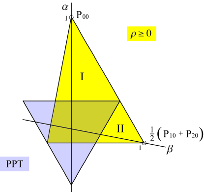
Figure 3: Illustration of the two–qutrit states $\rho_{\alpha,\beta}$ (50) and their partial transposition. The regions I and II label the regions where the states are entangled, they are PPT and separable in the overlap with the region of PPT points. The PPT points become semipositive under partial transposition.

It is shown in Ref. Baumgartner et al. (2006) that the PPT states $\rho_{\alpha,\beta}$ are all separable states, thus there exist no PPT entangled or bound entangled states of the form (50). Bound entanglement we detect for states that need more than two parameters in the Bell state expansion (see Secs. III.4.2 and III.4.3).

To find the HS measure for the entangled two–parameter two–qutrit states we apply the same procedure as in Sec. III.2: we determine the states that are the nearest separable ones in the Euclidean sense of Fig. 3 and use Lemma 1 to check whether these are indeed the nearest separable ones with respect to the whole state space (for other approaches see, e.g., Refs. Verstraete et al. (2002); Cao and Wang (2007)).

III.3.1 Region I

First, we consider Region I in Fig. 3, i.e., the triangle region of entangled states around the $\alpha$-axis, constrained by the parameter values

$$\alpha\;\leq\;\frac{7}{2}\beta+1,\quad\;\alpha\leq-\beta+1,\quad\;\alpha>\frac{\beta}{8}+\frac{1}{4}\,.$$ (55)

In the Euclidean picture, the point that is nearest to point $(\alpha,\beta)$ in this region is given by $(\frac{1}{4}+\frac{1}{8}\beta,\beta)$, which corresponds to the separable two–qutrit state

$$\tilde{\rho}_{\beta}\;=\;\frac{1}{9}\left(\mathbbm{1}\,+\,\left(\frac{1}{4}-\frac{3}{8}\beta\right)U_{1}\,+\,\left(\frac{1}{4}+\frac{9}{8}\beta\right)U_{2}\right)\,,$$ (56)

with $U_{1}$ and $U_{2}$ defined in Eq. (III.3).

For the difference of “nearest Euclidean separable” and entangled state, we find

$$\tilde{\rho}_{\beta}-\rho^{\rm{ent}}_{\alpha,\beta}\;=\;\frac{1}{9}\left(\frac{1}{4}+\frac{1}{8}\beta-\alpha\right)U\,,$$ (57)

where $U=U_{1}+U_{2}$ (defined in Eq. (9)). Using for the norm $\|U\|=3\sqrt{8}=6\sqrt{2}$ we gain the HS distance

$$\|\tilde{\rho}_{\beta}-\rho_{\alpha,\beta}^{\rm{ent}}\|\;=\;\frac{2\sqrt{2}}{3}\left(\alpha-\frac{1}{4}-\frac{1}{8}\beta\right)\,.$$ (58)

It remains to calculate

$$\langle\tilde{\rho}_{\beta},\tilde{\rho}_{\beta}-\rho_{\alpha,\beta}\rangle\;=\;\textnormal{Tr}\,\tilde{\rho}_{\beta}(\tilde{\rho}_{\beta}-\rho_{\alpha,\beta})\;=\;-\frac{2}{9}\left(\alpha-\frac{1}{4}-\frac{1}{8}\beta\right)$$ (59)

to set up the operator

$$\tilde{C}\;=\;\frac{\tilde{\rho}_{\beta}-\rho^{\rm{ent}}_{\alpha,\beta}\,-\,\langle\tilde{\rho}_{\beta},\tilde{\rho}_{\beta}-\rho^{\rm{ent}}_{\alpha,\beta}\rangle\,\mathbbm{1}}{\|\tilde{\rho}_{\beta}-\rho_{\alpha,\beta}^{\rm{ent}}\|}\;=\;\frac{1}{6\sqrt{2}}\,\left(2\,\mathbbm{1}\,-\,U\right)\,.$$ (60)

We test now whether it represents an entanglement witness, i.e., whether $\tilde{C}$ (60) satisfies the inequalities (III.1). As expected, we find

$$\langle\rho^{\rm{ent}}_{\alpha,\beta},\tilde{C}\rangle\;=\;-\frac{2\sqrt{2}}{3}\left(\alpha-\frac{1}{4}-\frac{1}{8}\beta\right)\;<\;0\,.$$ (61)

To check the second condition of inequalities (III.1) we set up the following Lemma, similar to Lemma 2.

Lemma 3.

For any Hermitian operator $C$ of a bipartite Hilbert-Schmidt space of dimension $d\times d$ that is of the form

$$C\;=\;a\left((d-1)\,\mathbbm{1}_{\rm{d^{2}}}\,+\,\sum_{n,m=0}^{d-1}c_{nm}\,U_{nm}\otimes U_{-nm}\right),\quad a\in\mathbbm{R}^{+},\ c_{nm}\in\mathbbm{C}$$ (62)

the expectation value for all separable states is positive,

$$\langle\rho,C\rangle\,\geq\,0\quad\forall\,\rho\in S\,,\quad\mbox{{if}}\quad|c_{nm}|\,\leq\,1\quad\forall\,n,m\,.$$ (63)

Proof. Any bipartite separable state can be decomposed into Weyl operators as

$$\rho\;=\; \sum_{k}p_{k}\ \frac{1}{d^{2}}\Big{(}\mathbbm{1_{\rm{d}}}\otimes\mathbbm{1_{\rm{d}}}\,+\,\sum_{n,m=0}^{d-1}\sqrt{d-1}\,n_{nm}^{k}\,U_{nm}\otimes\mathbbm{1_{\rm{d}}}\,+\,\sum_{l,k=0}^{d-1}\sqrt{d-1}\,m_{lk}^{k}\,\mathbbm{1_{\rm{d}}}\otimes U_{lk}$$

$$+\sum_{n,m,l,k=0}^{d_{1}-1}(d-1)\,n_{nm}^{k}m_{lk}^{k}U_{nm}\otimes U_{lk}\Big{)}\,,$$

$$n_{nm}^{k},m_{lk}^{k}\in\mathbbm{C}\,,\;\quad\left|\vec{n}^{k}\right|\leq 1\,,\quad\left|\vec{m}^{k}\right|\leq 1\,,\quad\ p_{k}\geq 0,\;\sum_{k}p_{k}=1\,,$$ (64)

where we define $\left|\vec{n}^{k}\right|^{2}:=\sum_{nm}n_{nm}^{*}n_{nm}=\sum_{nm}|n_{nm}|^{2}$.

Performing the trace, we obtain (keeping notation $\rho^{\dagger}$ formula (65) becomes more evident)

$$\langle\rho,C\rangle\;=\;\textnormal{Tr}\rho^{\dagger}\,C\;=\;\sum_{k}p_{k}\left((d-1)a\left(1\,+\,\sum_{n,m}c_{nm}n_{nm}^{*k}m_{-nm}^{*k}\right)\right)\,,$$ (65)

and using the restriction $|c_{nm}|\,\leq\,1\;\;\forall\,n,m$ we have

$$\left|\sum_{n,m}c_{nm}n_{nm}^{*k}m_{-nm}^{*k}\right|\;\leq\;\sum_{n,m}|n_{nm}^{k}||m_{-nm}^{k}|\;\leq\;1\,,$$ (66)

and since the convex sum of positive terms stays positive we get $\langle\rho,C\rangle\;\geq\;0\;\;\forall\rho\in S\,.\ \Box$

Since the operator $\tilde{C}$ (60) is of the form (62) we can use Lemma 3 to verify

$$\langle\rho,\tilde{C}\rangle\;\geq\;0\qquad\forall\rho\in S\,.$$ (67)

Thus $\tilde{C}$ (60) is indeed an entanglement witness and $\tilde{\rho}_{\beta}$ is the nearest separable state $\tilde{\rho}_{\beta}=\rho_{0;\,\beta}$ for the entangled states $\rho_{\alpha,\beta}^{\rm{ent}}$ in Region I.

For the HS measure of the entangled two–parameter two–qutrit states (50) we find

$$D^{I}(\rho_{\alpha,\beta}^{\rm{ent}})\;=\;\|\rho_{0;\,\beta}-\rho_{\alpha,\beta}^{\rm{ent}}\|\;=\;\frac{2\sqrt{2}}{3}\left(\alpha-\frac{1}{4}-\frac{1}{8}\beta\right)\,.$$ (68)

III.3.2 Region II

In Region II of Fig. 3, the entangled two–parameter two–qutrit states are constrained by

$$\alpha\;<\;\frac{5}{4}\beta-\frac{1}{2},\quad\;\alpha\;\geq\;\frac{1}{8}\beta-\frac{1}{8},\quad\;\alpha\;\leq\;-\beta+1\,.$$ (69)

The points that have minimal Euclidean distance to the points $(\alpha,\beta)$ located in this region are

$$\left(\begin{array}[]{c}\tilde{\alpha}\\ \tilde{\beta}\end{array}\right)=\left(\begin{array}[]{c}1/24\,\left(-2+20\alpha+5\beta\right)\\ 1/6\,\left(2+4\alpha+\beta\right)\end{array}\right)\,,$$ (70)

and correspond to the states $\tilde{\rho}_{\alpha,\beta}$. The quantities needed for calculating $\tilde{C}$ are

$$\tilde{\rho}_{\alpha,\beta}\,-\,\rho_{\alpha,\beta}^{\rm{ent}} \;=\; -\frac{1}{72}\left(4\alpha+2-5\beta\right)\left(U_{1}-U_{2}\right)\,,$$ (71)

$$\|\tilde{\rho}_{\alpha,\beta}-\rho_{\alpha,\beta}^{\rm{ent}}\| \;=\; \frac{1}{6\sqrt{2}}\left(-4\alpha-2+5\beta\right)\,,$$ (72)

$$\langle\tilde{\rho}_{\alpha,\beta},\tilde{\rho}_{\alpha,\beta}^{\rm{ent}}-\rho_{\alpha,\beta}\rangle \;=\; \frac{1}{36}\left(4\alpha+2-5\beta\right)\,,$$ (73)

so that operator $\tilde{C}$ is expressed by

$$\tilde{C}\;=\;\frac{1}{6\sqrt{2}}\,\left(2\,\mathbbm{1}\,+\,U_{1}\,-\,U_{2}\right)\,.$$ (74)

The check of the first of conditions (III.1) for an entanglement witness gives, unsurprisingly,

$$\langle\rho_{\alpha,\beta}^{\rm{ent}},\tilde{C}\rangle\;=\;\frac{1}{6\sqrt{2}}\,\left(4\alpha+2-5\beta\right)\,<\,0\,,$$ (75)

since $4\alpha<5\beta-2\,$, Eq. (69). For the second test we use the fact that operator $\tilde{C}$ (74) is of the form (62) and thus, according to Lemma 3, we obtain

$$\langle\rho,\tilde{C}\rangle\;\geq\;0\qquad\forall\rho\in S\,.$$ (76)

Therefore, $\tilde{C}$ (74) is indeed an entanglement witness and the states $\tilde{\rho}_{\alpha,\beta}$ are the nearest separable ones $\tilde{\rho}_{\alpha,\beta}=\rho_{0;\,\alpha,\beta}$ to the entangled two–parameter states (50) of Region II.

Finally, for the HS measure of these states, we find

$$D^{II}(\rho_{\alpha,\beta}^{\rm{ent}})\;=\;\|\rho_{0;\,\alpha,\beta}\,-\,\rho_{\alpha,\beta}^{\rm{ent}}\|\;=\;\frac{1}{6\sqrt{2}}\,\left(-4\alpha-2+5\beta\right)\,.\\$$ (77)

Another way to arrive at the nearest separable states for the two–parameter states is to calculate the nearest PPT states with the method of Ref. Verstraete et al. (2002) first and then check if the gained states are separable. If we do so we obtain for the nearest PPT states the states $\tilde{\rho}_{\beta}$ and $\tilde{\rho}_{\alpha,\beta}$ we found with our “guess method”, we know from Ref. Baumgartner et al. (2006) these states are separable and therefore they have to be the nearest separable states.

III.4 Three–parameter entangled states and bound entanglement — qutrits

III.4.1 Detecting bound entanglement with geometric entanglement witnesses

As we already mentioned, the PPT-criterion Peres (1996); Horodecki et al. (1996) is a necessary criterion for separability (and sufficient for $2\times 2$ or $2\times 3$ dimensional Hilbert spaces). A separable state has to stay positive semidefinite under partial transposition. Thus, if a density matrix becomes indefinite under partial transposition, i.e. one or more eigenvalues are negative, it has to be entangled and we call it a NPT entangled state. But there exist entangled states that remain positive semidefinite – PPT entangled states – these are called bound entangled states, since they cannot be distilled to a maximally entangled state Horodecki (1997); Horodecki et al. (1998).

Let us consider states on a $d_{1}\times d_{2}$ dimensional Hilbert space, $D:=d_{1}d_{2}$. The set of all PPT states $P$ is convex and compact and contains the set of separable states. Thus in Eq. (11) the nearest separable state $\rho_{0}$ can be replaced by the nearest PPT state $\tau_{0}$ for which the minimal distance to the set of PPT states is attained,

$$\min_{\tau\in P}\|\tau-\rho\|\;=\;\|\tau_{0}-\rho\|\,.$$ (78)

If $\rho$ is a NPT entangled state $\rho_{\rm{NPT}}$ and $\tau_{0}$ the nearest PPT state, then the operator

$$A_{\rm{PPT}}\;:=\;\tau_{0}\,-\,\rho_{\rm{NPT}}\,-\,\langle\tau_{0},\tau_{0}-\rho_{\rm{NPT}}\rangle\,\mathbbm{1}_{\rm{D}}$$ (79)

defines a tangent hyperplane to the set $P$ for the same geometric reasons as operator (14) and has to be an entanglement witness since $P\supset S$ (for convenience we do not normalize (79) since it does not affect the following calculations). The nearest PPT state $\tau_{0}$ can be found using the method provided in Ref. Verstraete et al. (2002). In principle, the entanglement of $\rho_{\rm{NPT}}$ can be measured in experiments that should verify Tr$A_{\rm{PPT}}\,\rho_{\rm{NPT}}<0$. If the state $\tau_{0}$ is separable, it has to be the nearest separable state $\rho_{0}$ since the operator (79) defines a tangent hyperplane to the set of separable states. Therefore, in this case, $A_{\rm{PPT}}$ is an optimal entanglement witness, $A_{\rm{PPT}}=A_{\rm{opt}}$, and the HS measure of entanglement can be readily obtained. If $\tau_{0}$ is not separable, that is PPT and entangled, it has to be a bound entangled state.

Unfortunately, it is not trivial to check if the state $\tau_{0}$ is separable or not. As already mentioned, it is hard to find evidence of separability, but it might be easier to reveal bound entanglement, not only for the state $\tau_{0}$ but for a whole family of states. A method to detect bound entangled states we are going to present now.

Consider any PPT state $\rho_{\rm{PPT}}$ and the family of states $\rho_{\lambda}$ that lie on the line between $\rho_{\rm{PPT}}$ and the maximally mixed (and of course separable) state $\frac{1}{D}\mathbbm{1}_{\rm{D}}$,

$$\rho_{\lambda}\;:=\;\lambda\,\rho_{\rm{PPT}}\,+\,\frac{(1-\lambda)}{D}\,\mathbbm{1}_{\rm{D}}\,.$$ (80)

We can construct an operator $C_{\lambda}$ in the following way:

$$C_{\lambda}\;=\;\rho_{\lambda}\,-\,\rho_{\rm{PPT}}\,-\,\langle\rho_{\lambda},\rho_{\lambda}-\rho_{\rm{PPT}}\rangle\,\mathbbm{1}_{\rm{D}}\,.$$ (81)

If we can show that for some $\lambda_{\rm{min}}<1$ we have $\textnormal{Tr}\,\rho\,C_{\lambda_{\rm{min}}}\geq 0$ for all $\rho\in S$, $C_{\lambda_{\rm{min}}}$ is an entanglement witness (due to the construction of $C_{\lambda}$ the condition Tr $\rho_{\lambda}C_{\lambda}<0$ is already satisfied) and therefore $\rho_{\rm{PPT}}$ and all states $\rho_{\lambda}$ with $\lambda_{\rm{min}}<\lambda\leq 1$ are bound entangled (see Fig. 4). In Ref. Bandyopadhyay et al. (2008) a similar approach is used to identify bound entangled states in the context of the robustness of entanglement.

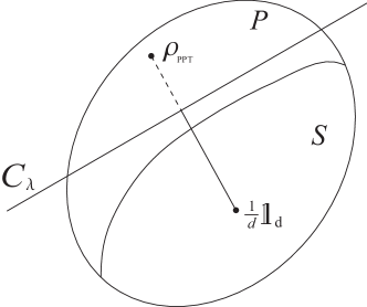
Figure 4: Sketch of the presented method to detect bound entanglement with the geometric entanglement witness $C_{\lambda}$. The dashed line indicates the detected bound entangled states $\rho_{\lambda}$ ($\lambda_{\rm{min}}<\lambda\leq 1$), states $\rho_{\lambda}$ with $0<\lambda\leq\lambda_{\rm{min}}$ can be separable or bound entangled (straight line).

III.4.2 Application of the method to detect bound entanglement

Let us now introduce the following family of three–parameter two–qutrit states:

$$\rho_{\alpha,\beta,\gamma}\;:=\;\frac{1-\alpha-\beta-\gamma}{9}\,\mathbbm{1}\,+\,\alpha P_{00}\,+\,\frac{\beta}{2}\left(P_{10}+P_{20}\right)\,+\,\frac{\gamma}{3}\left(P_{01}+P_{11}+P_{21}\right)\,,$$ (82)

where the parameters are constrained by the positivity requirement $\rho_{\alpha,\beta,\gamma}\geq 0$,

$$\alpha\; \leq\;\frac{7}{2}\beta+1-\gamma\,,\quad \alpha\; \leq\;-\beta+1-\gamma\,,$$

$$\alpha\; \leq\;-\beta+1+2\gamma\,,\quad \alpha\; \geq\;\frac{\beta}{8}-\frac{1}{8}+\frac{1}{8}\gamma\,.$$ (83)

States (82) lie again in the magic simplex and for $\gamma=0$ we come back to the states (50) considered before. However, for $\gamma\neq 0$ it is not trivial to find the nearest separable states since the PPT states do not necessarily coincide with the separable states. But we can use our geometric entanglement witness (81) to detect bound entanglement (see Refs. Bertlmann and Krammer (2008b, c)).

We start with the following one–parameter family of two–qutrit states that was introduced in Ref. Horodecki et al. (1999):

$$\rho_{b}\;=\;\frac{2}{7}\left|\phi_{+}^{3}\right\rangle\left\langle\phi_{+}^{3}\right|\,+\,\frac{b}{7}\,\sigma_{+}\,+\,\frac{5-b}{7}\,\sigma_{-}\,,\qquad 0\leq b\leq 5\,,$$ (84)

where

$$\sigma_{+}\;:=\;\ \frac{1}{3}\left(\left|01\right\rangle\left\langle 01\right|\,+\,\left|12\right\rangle\left\langle 12\right|\,+\,\left|20\right\rangle\left\langle 20\right|\,\right)\,,$$ (85)

$$\sigma_{-}\;:=\;\ \frac{1}{3}\left(\left|10\right\rangle\left\langle 10\right|\,+\,\left|21\right\rangle\left\langle 21\right|\,+\,\left|02\right\rangle\left\langle 02\right|\,\right)\,.$$ (86)

Let us call this family of states Horodecki states. Interestingly, the states (84) are part of the three–parameter family (82), namely

$$\rho_{b}\;\equiv\;\rho_{\alpha,\beta,\gamma}\qquad\mbox{with}\quad\alpha=\frac{6-b}{21},\;\beta=-\frac{2b}{21},\;\gamma=\frac{5-2b}{7}\,,$$ (87)

and thus lie in the magic simplex. Testing the partial transposition, we find that the Horodecki states (84) split the states in the following way: for $0\leq b<1$ they are NPT, for $1\leq b\leq 4\,$ PPT and for $4<b\leq 5\,$ NPT. In Ref. Horodecki et al. (1999), it is shown that the states are separable for $2\leq b\leq 3$ and bound entangled for $3<b\leq 4\,$. In our case, it is more convenient to use $\gamma$ as the parameter of the Horodecki states. Using Eq. (87) we express $b$ in terms of $\gamma$ and obtain

$$\rho_{b}\;\equiv\;\rho_{\alpha,\beta,\gamma}\qquad\mbox{with}\quad\alpha=\frac{1+\gamma}{6},\beta=\frac{-5+7\gamma}{21},\gamma\,.$$ (88)

The geometry of the three–parameter family of states $\rho_{\alpha,\beta,\gamma}$ as part of the magic simplex we show in Fig. 5,

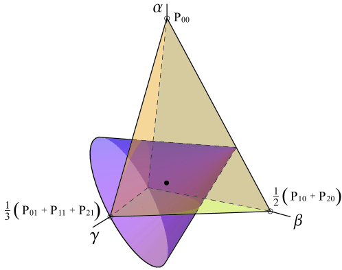
Figure 5: The states $\rho_{\alpha,\beta,\gamma}$ represent a pyramid with a triangular base due to the positivity constraints (III.4.2) and the PPT points with constraints (III.4.2) form a cone which overlaps with the pyramid. The bound entangled and separable states lie in the intersection region. The black dot indicates the maximally mixed state and the origin of the non–orthogonal coordinate axes.

in particular, the states $\rho_{\alpha,\beta,\gamma}$ with positivity requirement (III.4.2) and the PPT states which are constrained by

$$\alpha \;\leq\; -\beta-\frac{1}{2}+\frac{1}{2}\gamma\,,$$

$$\alpha \;\leq\; \frac{1}{16}\left(-2+11\beta+3\sqrt{\Delta}\right)\,,\;\quad\alpha\;\leq\;\frac{1}{16}\left(-2+11\beta-3\sqrt{\Delta}\right)\,,$$ (89)

where $\Delta=4+9\beta^{2}+4\gamma-7\gamma^{2}-6\beta(2+\gamma)$. The states $\rho_{\alpha,\beta,\gamma}$ form due to the positivity constraints (III.4.2) a pyramid with triangular base and the PPT points due to the constraints (III.4.2) a cone. Both objects are quite symmetric and overlap with each other in a way shown in Fig. 5. In the intersection region lie the bound entangled and separable states.

Application of the method. We now want to apply the method to detect bound entanglement of the three–parameter family (82). The idea is to choose PPT starting points on the boundary plane $\alpha=\frac{7}{2}\beta+1-\gamma$ of the positivity pyramid, on the Horodecki line and in a region close to this line, and shift the operators $C_{\lambda}$ along the parameterized lines that connect the starting points with the maximally mixed states. If we can show that $C_{\lambda}$ is an entanglement witness until a certain $\lambda_{min}$, all states $\rho_{\lambda}$ (80) with $1\leq\lambda<\lambda_{min}$ are PPT entangled.

We parameterize our “starting states” on the boundary plane by

$$\rho_{\rm{plane}}\;\equiv\;\rho_{\alpha,\beta,\gamma}\quad\mbox{with}\quad\left(\alpha=\frac{1+\gamma+\epsilon}{6}\,,\beta=\frac{-5+7\gamma+\epsilon}{21}\,,\gamma\right),\quad\epsilon\in\mathbbm{R}\,,$$ (90)

where we introduced an additional parameter $\epsilon$ to account for the deviation from the line within the boundary plane.

Depending on $\gamma$ and $\epsilon$ the operator $C_{\gamma,\epsilon,\lambda}$ (81) has the following form:

$$C_{\gamma,\lambda}\,\;=\;\,\rho_{\lambda}\,-\,\rho_{pl}\,-\,\langle\rho_{\lambda},\rho_{\lambda}-\rho_{pl}\rangle\,\mathbbm{1}\,\;=\;\,a\,(2\,\mathbbm{1}\,+\,c_{1}U_{1}\,+\,c_{2}U^{I}_{2}\,+\,c^{\star}_{2}U^{II}_{2})\,,$$

$$\mbox{with}\quad a\;=\;\frac{d}{36}\,\lambda(1-\lambda)\,,\quad d\;=\;1+3\gamma^{2}+3\epsilon(2+\epsilon)/7\,,$$

$$c_{1}\;=\;-\frac{4(2+\epsilon)}{7d\lambda}\,,\quad c_{2}\;=\;\frac{2(1-7\sqrt{3}\gamma\,i-3\epsilon)}{7d\lambda}\,.$$ (91)

The operators $U_{1},U^{I}_{2},U^{II}_{2}$ are defined by Eq. (III.3) and the family of states $\rho_{\lambda}$ by

$$\rho_{\lambda}\;=\;\lambda\,\rho_{\rm{plane}}\,+\,\frac{1-\lambda}{9}\,\mathbbm{1}\,.$$ (92)

We want to find the minimal $\lambda$, denoted by $\lambda_{\rm{min}}$, depending on the parameters $\gamma$ and $\epsilon\,$, such that all states on the line (92) are bound entangled for $\lambda_{\rm{min}}<\lambda\leq 1$. To accomplish this, we define the functions

$$g_{1}(\gamma,\epsilon,\lambda)\;:=\;|c_{1}|\quad\mbox{and}\quad g_{2}(\gamma,\epsilon,\lambda)\;:=\;|c_{2}|\,,$$ (93)

then $\lambda_{\rm{min}}$ is attained at $\max\{g_{1}(\gamma,\epsilon,\lambda),g_{2}(\gamma,\epsilon,\lambda)\}=1$ (recall Lemma 3). Bound entanglement can be found in a region where $\lambda_{\rm{min}}<1$ and the starting points of the lines (92) are PPT states. That means, $\epsilon$ and $\gamma$ are chosen such that the starting points are PPT states and the corresponding line allows a $\lambda_{\rm{min}}<1$. The parameter $\epsilon$ is bounded by $-1/4<\epsilon<1/3\,$, where the lower bound is reached for $\lambda_{\rm{min}}\rightarrow 1$ at $|\gamma|=1/4$ and the upper bound arises from the boundary of the PPT states at $\gamma=0$. For every $\epsilon$ in this interval, we have an interval of $|\gamma|$ where bound entangled states are located.

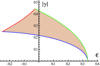
Figure 6: Plot of the parameter range $\gamma$ versus $\epsilon$ of starting points of the lines (92) such that bound entangled states can be detected.

More precisely, in the interval for the $\epsilon$ parameter $-1/4<\epsilon<\epsilon_{0}\,$ with $\epsilon_{0}=\left(8\,-\,7\,(2/(-5+\sqrt{29}))^{1/3}\,+\,7\,(2/(-5+\sqrt{29}))^{-1/3}\right)/\,3\;\simeq\;-\,0.03\,$ the parameter $\gamma$ is confined by $\sqrt{1-2\epsilon+3\epsilon^{2}}\,/\sqrt{21}<|\gamma|<\sqrt{7-6\epsilon-3\epsilon^{2}-2\,(1-48\epsilon-12\epsilon^{2})^{1/2}}\,/\sqrt{21}\,$, under the constraint $\lambda_{\rm{min}}<1$. For the remaining interval $\epsilon_{0}<\epsilon<1/3\,$, we get the bounds $\sqrt{1-2\epsilon+3\epsilon^{2}}\,/\sqrt{21}<|\gamma|<\sqrt{9-26\epsilon-3\epsilon^{2}}\,/\,7\,$, where the lower bound is again constrained by $\lambda_{\rm{min}}<1$ and the upper one by the PPT condition. A plot of the allowed values of $\epsilon$ and $\gamma$ for the starting points on the boundary plane is depicted in Fig. 6. We have equality of the coefficient functions $g_{1}=g_{2}$ for $|\gamma|=\sqrt{15+22\epsilon-5\epsilon^{2}}\,/\,7\sqrt{3}=:\gamma_{0}\,$, $g_{1}>g_{2}$ for $|\gamma|<\gamma_{0}$ and $g_{1}<g_{2}$ for $|\gamma|>\gamma_{0}$, where $|\gamma|$ is always restricted to the allowed range described above. As mentioned, $\lambda_{\rm{min}}$ is gained from the condition $\max\{g_{1}(\gamma,\epsilon,\lambda),g_{2}(\gamma,\epsilon,\lambda)\}=1$ for particular values of $\gamma$ and $\epsilon$. The total minimum $\lambda_{\rm{min}}^{\rm{tot}}$ is finally reached at

$$\lambda_{\rm{min}}^{\rm{tot}}\;=\;\frac{1}{8}\,(3+\sqrt{13})\;\simeq\;0.826\,,$$ (94)

which is significantly below the value $1$ so that the resulting volume of bound entangled states is remarkably large. The total minimum (94) is attained at $\epsilon=(7\sqrt{13}-25)\,/\,2\;\simeq\;0.12$ and $|\gamma|\;\simeq\;0.35\,$. The whole line of states $\rho_{\lambda}$ (92) within the interval $\lambda_{\rm{min}}^{\rm{tot}}<\lambda\leq 1$ is found to be bound entangled. The volume of the detected bound entangled states we have visualized in Fig. 7. For $\gamma=0$ no bound entanglement occurs, as discussed in Sec. III.3, which is represented in Fig. 7 at the meeting point of the two bound entangled regions.

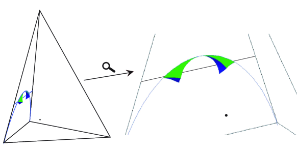
Figure 7: Regions of detected bound entangled states within the pyramid represented by the three–parameter states $\rho_{\alpha,\beta,\gamma}$ (82). The dot represents the maximally mixed state, the Horodecki states are represented by the line through the boundary plane from which the regions of bound entanglement emerge. In the magnified picture on the right hand side the viewpoint is altered a bit to gain a better visibility.

III.4.3 More bound entangled states and the shape of separable states

In the last section, we gave a strict application of our method to detect bound entangled states, where we recognized bound entangled states on the parameterized lines $\rho_{\lambda}$ (80) only. The involved entanglement witnesses, however, are able to detect the entanglement of all states on one side of the corresponding plane, not only on the lines. Therefore even larger regions of bound entanglement can be identified for the three–parameter family (82), which is described in detail in Ref. Bertlmann and Krammer (2008c).

In this subsection, we want to show that for the three–parameter family (82) our method detects the same bound entangled states as the realignment criterion does, and furthermore allows for a construction of the shape of the separable states of the three–parameter family, so that we are able to fully determine the entanglement properties of this family of states.

The realignment criterion is a necessary criterion of separability and says that for any separable state the sum of the singular values $s_{i}$ of a realigned density matrix $\sigma_{R}$ has to be smaller than or equal to one,

$$\sum_{i}s_{i}\;=\;\textnormal{Tr}\sqrt{\sigma^{\dagger}_{R}\sigma_{R}}\;\leq\;1\,,$$ (95)

where $\left(\rho_{ij,kl}\right)_{R}:=\rho_{ik,jl}$ (for details see Refs. Rudolph (2000, , 2003); Chen and Wu (2003)). States that violate the criterion have to be entangled, states that satisfy it can be entangled or separable.

In our case of the three–parameter family (82) we obtain the constraints

$$\alpha\;\leq\; \ \frac{1}{16}\left(6+11\beta-\gamma-\Delta_{1}\right)$$ (96)

$$\alpha\;\leq\; \ \frac{1}{16}\left(6+11\beta-\gamma+\Delta_{1}\right)$$ (97)

$$\alpha\;\geq\; \ \frac{1}{16}\left(-6+11\beta-\gamma-\Delta_{2}\right)$$ (98)

$$\alpha\;\geq\; \ \frac{1}{16}\left(-6+11\beta-\gamma+\Delta_{2}\right)$$ (99)

from the realignment criterion, where

$$\Delta_{1}\;:=\; \ \sqrt{4+36\beta+81\beta^{2}-12\gamma-54\beta\gamma+33\gamma^{2}}\qquad\mbox{and}$$

$$\Delta_{2}\;:=\; \ \sqrt{4-36\beta+81\beta^{2}+12\gamma-54\beta\gamma+33\gamma^{2}}.$$ (100)

Only constraint (96) is violated by some PPT states, which thus have to be bound entangled. The PPT entangled states exposed by the realignment criterion are therefore concentrated in the region confined by the constraints

$$\alpha\;\leq\;\frac{7}{2}\beta+1-\gamma,\;\ \alpha\;\leq\;\frac{1}{16}\left(-2+11\beta+3\sqrt{\Delta}\right),\;\ \alpha\;\geq\;\ \frac{1}{16}\left(6+11\beta-\gamma-\Delta_{1}\right)\,.$$ (101)

All PPT entangled states of Eq. (101) can also be detected using Lemma 3. To see this, we construct tangent planes onto the surface of the function

$$\alpha\;=\;\ \frac{1}{16}\left(6+11\beta-\gamma-\Delta_{1}\right)$$ (102)

from the realignment criterion (96), where we use orthogonal coordinates. In this way, we can assign geometric operators to the tangential planes by choosing points $\vec{a}$ inside the planes and points $\vec{b}$ outside the planes such that $\vec{a}-\vec{b}$ is orthogonal to the planes. Since the Euclidean geometry of our picture is isomorph to the Hilbert-Schmidt geometry, the points $\vec{a}$ and $\vec{b}$ correspond to states $\rho_{a}$ and $\rho_{b}$ and we can construct an operator accordingly,

$$C_{\rm{re}}\;=\;\rho_{a}-\rho_{b}\;-\;\langle\rho_{a},\rho_{a}-\rho_{b}\rangle\mathbbm{1}_{9}\,.$$ (103)

Decomposed into the Weyl operator basis, the operators (103) that correspond to tangent planes in points $(\alpha_{\rm t},\beta_{\rm t},\gamma_{\rm t})$ – where $\alpha_{\rm t}$ is a function of $\beta_{\rm t}$ and $\gamma_{\rm t}$, given by the realignment function (102) – are

$$C_{\rm{re}}\;=\; \ a\,(2\,\mathbbm{1}-U_{1}+c\,U^{I}_{2}\,+\,c^{*}U^{II}_{2})\,,\quad\mbox{with}$$

$$a\;=\;\frac{1}{36}\left(-2-9\beta_{\rm t}+3\gamma_{\rm t}+3\Delta_{c}\right),$$

$$c\;=\;\frac{9\gamma_{\rm t}^{2}+(-2-9\beta_{\rm t}+3\gamma_{\rm t})\Delta_{c}+\sqrt{3}\gamma_{\rm t}\left(2+9\beta_{\rm t}-3\gamma_{\rm t}+3\Delta_{c}\right)i}{(2+9\beta_{\rm t})^{2}-6(2+9\beta_{\rm t})\gamma_{\rm t}+36\gamma_{\rm t}^{2}}\,,$$

$$\Delta_{c}\;:=\;\sqrt{4+36+81\beta_{\rm t}^{2}-12\gamma_{\rm t}-54\beta_{\rm t}\gamma_{\rm t}+33\gamma_{\rm t}^{2}}\;.$$ (104)

The absolute values of the coefficients $c$ and $c^{*}$ in Eq. (III.4.3) are $1$, $|c|=|c^{*}|=1$, and therefore, according to Lemma 3, the operators $C_{\rm{re}}$ are entanglement witnesses that detect the entanglement of all states “above” the corresponding planes, thus also the bound entangled states in the region of Eq. (101). The detected bound entangled region is depicted in Fig. 8.

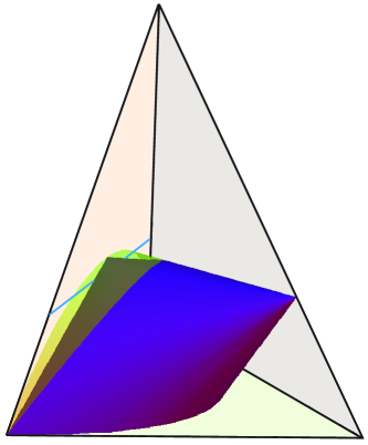
Figure 8: Illustration of the PPT and realignment criteria. The familiar PPT cone (here pictured only inside the positivity pyramid) is intersected by a cone formed by the realignment constraint (96) and reveals a region of bound entangled states (translucent yellow region) that can also be detected by Lemma 3.

Naturally, now the question arises if all the states $\rho_{\alpha,\beta,\gamma}$ (82) that satisfy both the PPT and the realignment criterion are separable. This cannot be seen using the two criteria alone, since they are not sufficient criteria for separability. But we can apply a method of shifting operators along parameterized lines in the other direction: by constructing a kernel polytope of necessarily separable states and assigning operators to the boundary planes of this polytope, we can shift those operators outside until they become entanglement witnesses, which can be shown numerically (unfortunately Lemma 3 does not help here). In this way, one can step by step reconstruct the shape of the separable states, which indeed is the set given by the states that satisfy the PPT and the realignment criterion (see dark shape of the two intersecting cones in Fig. 8); for details see Ref. Krammer (2009). Hence, we see that the presented method of “shifting” operators along parameterized lines does not only help to detect bound entanglement, but also to construct the shape of the separable states.

IV Conclusion

We discuss the geometric aspects of entanglement for density matrices within a simplex formed by Bell states. We use entanglement witnesses in order to quantify entanglement and detect in case of qutrits bound entangled states in specific instances.

We demonstrate the geometry of separability and entanglement in case of qubits by choosing so-called two–parameter states, Eq. (15), i.e., planes in the simplex, a tetrahedron (see Fig. 2). These states reflect already the underlying geometry of the Hilbert space and they are chosen with regard to the description of qutrit states, a generalization into higher dimensions. To a given entangled state we determine the nearest separable state, calculate the corresponding entanglement witness and the Hilbert–Schmidt measure in the relevant Regions I and II (see Fig. 1).

In case of qutrits it is quite illustrative to demonstrate the geometry of separability and entanglement in terms of two–parameter states (50). These states represent a plane in the eight–dimensional simplex formed by the nine Bell states, the magic simplex, and are easy to construct within the Weyl operator basis. Due to the high symmetry of this simplex we may restrict ourselves to a certain mixture of Bell states, Eq. (50), which lie on a line in a phase space description. This line exhibits the same geometry as other lines. Within the Weyl operator basis it is quite easy to find the Bloch vector form (51) of the two–parameter states. It enables us to find in regions I and II (see Fig. 3) the nearest separable state to a given entangled state and the corresponding entanglement witness. The easy calculation of the Hilbert–Schmidt measure of entanglement is a great advantage and its result of high interest. Other entanglement measures, like the entanglement of formation, are much harder to be calculated in this higher dimensional case.

We present a method to find analytically bound entangled states by using entanglement witnesses. These witnesses are constructed geometrically, Eq. (81), in quite the same way as for the detection of the nearest separable state, Eq. (14). We show that the Horodecki states (84) can be described by the family of three–parameter states (82) and are therefore part of the magic simplex. Geometrically, they form a line on the boundary of the pyramid represented by the three–parameter states (82) (see Figs. 7 and 8). We apply our method to find regions of bound entangled states within the pyramid of states (82) (see Fig. 7). Even when restricting ourselves strictly to consider the detected bound entangled states on the parameterized lines (80) only, we find large regions of bound entanglement. Employing the realignment criterion of separability, we can reveal larger regions of bound entanglement that are also detected by Lemma 3. Finally, we can apply our method of shifting operators along parameterized lines together with numerical calculations to show that there do not exist more PPT entangled states for the three–parameter family. Hence, the shape of the separable states can be constructed.

When decomposing density matrices into operator bases the Weyl operator basis is the optimal one for all our calculations. The reason is that entangled states – the maximally entangled Bell states – are in fact easily constructed by unitary operators à la Weyl, see Eq. (46).