Bloch oscillations of Bose-Einstein condensates: Quantum counterpart of dynamical instability

Abstract

We study the Bloch dynamics of a quasi one-dimensional Bose-Einstein condensate of cold atoms in a tilted optical lattice modeled by a Hamiltonian of Bose-Hubbard type: The corresponding mean-field system described by a discrete nonlinear Schrödinger equation can exhibit dynamical (or modulation) instability due to chaotic dynamics and equipartition over the quasimomentum modes. It is shown that these phenomena are related to Bogoliubov’s depletion of the Bose-Einstein condensate and a decoherence of the condensate in the many-particle description. Three types of dynamics are distinguished: (i) decaying oscillations in the region of dynamical instability, and (ii) persisting Bloch oscillations or (iii) periodic decay and revivals in the region of stability.

I Introduction

Recently, considerable attention has been paid to the dynamics of cold atoms and Bose-Einstein condensates (BECs) loaded into an optical lattice with a static, e.g., gravitational, force (see Daha96 ; Raiz97 and Ande98 ; Mors01 ; Cris02 ; Jona03 ; Ott04 ; 04bloch_bec ; Wimb05 ; Sias07 ; Gust08a ; Fatt08 ). In the limit of vanishing particle interaction the system shows Bloch oscillations (BO) (for a review see, e.g., 04bloch ). However, it is known that the interaction between the atoms leads to modifications and possibly even to a breakdown of these Bloch oscillations.

The most prominent theoretical approach to investigate the dynamics is the reduction of the many-particle system to a mean-field description via the (nonlinear) Gross-Pitaevskii equation. The description can be further simplified by discretizing it in terms of Wannier functions localized on the lattice sites. In the many-particle description this yields a Bose-Hubbard model and accordingly the mean-field dynamics is described by the discrete nonlinear Schrödinger equation (DNLSE) (see, e.g., Smer03 ). It should be pointed out that the mean-field approximation is formally equivalent to a classical limit for single particle quantum mechanics. Therefore, it is often denoted as ‘(pseudo)classical’, although it still describes a quantum system. This becomes evident in the limit of vanishing interaction, where it reduces to a single particle Schrödinger equation. Nevertheless, the formal similarity of the many-particle to mean-field transition and the quantum classical correspondence allows for the application of semiclassical methods as well as the investigation of topics such as quantum chaos within the framework of ultracold atoms Holt01a ; Moss06 ; Wu06 ; 07semiMP ; Luo08 ; 08kicked ; Weis08 .

The mean-field system of interest in the present study shows a rich structure of mixed and chaotic behavior and our main aim will be to identify the counterparts of some pronounced features in the corresponding many-particle system. For this purpose we compare the DNLSE dynamics with the underlying microscopic many-particle system, described by the 1D bosonic Hubbard model with the Hamiltonian

$$\widehat{H}=\sum_{l}\epsilon_{l}\hat{n}_{l}-\frac{J}{2}\sum_{l}\Big{(}\hat{a}^{\dagger}_{l+1}\hat{a}_{l}+h.c.\Big{)}+\frac{W}{2}\sum_{l}\hat{n}_{l}(\hat{n}_{l}-1)\;,$$ (1)

where $\hat{a}^{\dagger}_{l}$ and $\hat{a}_{l}$ are bosonic creation and annihilation operators for the $l$th lattice site, and $\hat{n}_{l}=\hat{a}^{\dagger}_{l}\hat{a}_{l}$ are the associated number operators. The hopping energy and the particle interaction are denoted by $J$ and $W$, respectively, and $\epsilon_{l}=dFl$ is the on-site energy where $d$ is the lattice period and $F$ the magnitude of a static force. Experimentally, all these quantities can be controlled separately. However, the validity of the Bose-Hubbard model is based on certain assumptions such as the single band tight binding approximation, which may break down in some parameter regions. Yet, for the following studies only the ratios of the quantities are of interest for the qualitative behavior of the system which offers an additional freedom to maintain the validity of the Bose-Hubbard Hamiltonian. Therefore, we believe that the observations reported in the following should be experimentally accessible.

The Hamiltonian commutes with $\hat{N}=\sum_{l}\hat{n}_{l}$ and therefore the total number $N$ of particles is conserved. Here we consider the macroscopic limit $N\rightarrow\infty$, $W\rightarrow 0$ with constant $g=WN/L$ where the number of sites, $L$, is kept finite. In this limit the mean-field approximation can be applied, which usually is formulated as replacing the bosonic operators $\hat{a}_{l}$, $\hat{a}^{\dagger}_{l}$ by complex numbers $a_{l}$, $a^{*}_{l}$, the components of an effective single particle wave function which appear as ‘classical’ canonical variables. The resulting mean-field Hamiltonian function is given by

$$H\!=\!\sum_{l}\epsilon_{l}|a_{l}|^{2}\!-\!\frac{J}{2}\sum_{l}\Big{(}a^{*}_{l+1}\,a_{l}+c.c.\Big{)}\!+\!\frac{g}{2}\sum_{l}|a_{l}|^{4}\,,$$ (2)

up to a term proportional to $\sum_{l}|a_{l}|^{2}$, which is an integral of motion. The DNLSE can be formulated via the canonical equations of motion

$$i\,\hbar\dot{a}_{l}=\partial H/\partial a^{*}_{l}\ ,\quad i\,\hbar\dot{a}_{l}^{*}=-\partial H/\partial a_{l}\,.$$ (3)

One aim of the present paper is to investigate the validity of this mean-field approach for a system with finite particle number in the different parameter regions.

For nonvanishing particle interaction $g\neq 0$ the mean-field Bloch oscillations are damped 04bloch_bec ; Wimb05 . In this context the main phenomena are the dynamical instability which is also known as modulation instability (see, e.g., Kolo04a ; Zhen04 ) and the equipartition over the quasimomentum modes (also denoted as thermalization) due to the onset of classical chaos in the DNLSE. On the other hand, within the many-particle approach the main phenomenon induced by the interaction is a decay of Bloch oscillations due to decoherence 04bloch ; 04bloch_bec . The present analysis shows a direct relation between these classical and quantum phenomena. We argue that the quantum manifestations of both dynamical instability and equipartition can be understood in terms of the depletion of the Floquet-Bogoliubov states, defined as the “low-energy” eigenstates of the evolution operator over one Bloch period.

We furthermore go beyond the traditional single trajectory mean-field treatment and, following a recent suggestion 07phase , average the dynamics over an ensemble of trajectories given by the Husimi distribution of the initial many-particle state. It is shown that this method is capable of describing important features of the many-particle dynamics.

The paper is organized as follows: In Sec. II we discuss the mean-field dynamics, in particular the stability properties of the Bloch oscillation and its relation to chaotic dynamics. The corresponding many-particle system is analyzed in Sec. III, mainly based on the Floquet-Bogoliubov states whose depletion properties provide a measure for the many-particle stability which can be compared to the mean-field behavior. We summarize our results and end with a short outlook in Sec. IV.

II Mean-field dynamics

Evaluating the canonical equations of motion (3) with the Hamiltonian function (2) yields the mean-field equations of motion of a BEC in a tilted optical lattice, the DNLSE:

$$i\;\hbar\dot{a}_{l}=\epsilon_{l}a_{l}-\frac{J}{2}(a_{l+1}+a_{l-1})+g|a_{l}|^{2}a_{l}\;,\quad\epsilon_{l}=dFl\,.$$ (4)

Here $a_{l}(t)$ are the complex amplitudes of a mini BEC associated with the $l$ th well of the optical potential, $J$ is the hopping or tunneling matrix element, $d$ the lattice period, $F$ the magnitude of the static force, and $g$ the nonlinear parameter, given by the product of the microscopic interaction constant $W$ and the filling factor $\bar{n}$ (the mean number of atoms per lattice site). It should be noted that Eq. (4) can also be derived as a tight-binding approximation for the discretized Gross-Pitaevskii equation. To simplify the equations we shall set the lattice period $d$ and the Planck constant $\,\hbar$ to unity in the following.

Throughout the paper we shall use the gauge transformation

$$a_{l}(t)\rightarrow\exp[-i(g+Fl)t]a_{l}(t)\,$$ (5)

that eliminates the static term in Eq. (4). Note that the inclusion of $g$ in the transformation is optional and is done to facilitate the stability analysis below. The effect of the static force then appears as periodic driving of the system with the Bloch frequency $F$:

$$i\dot{a}_{l}=-\frac{J}{2}\left(e^{-iFt}a_{l+1}+e^{+iFt}a_{l-1}\right)+g\left(|a_{l}|^{2}-1\right)a_{l}\;.$$ (6)

An advantage of the gauge transformation is that one can impose periodic boundary conditions, $a_{0}(t)\equiv a_{L}(t)$, where we restrict ourselves to odd values of $L$. Equation (6) also appears as a canonical equation of motion generated by the Hamiltonian function

$$H(t)=-\frac{J}{2}\sum_{l}\left(e^{iFt}a^{*}_{l+1}a_{l}+c.c.\right)+\frac{g}{2}\sum_{l}|a_{l}|^{2}\big{(}|a_{l}|^{2}-2\big{)}\,.$$ (7)

In this work, we shall be concerned mainly with almost uniform initial conditions $a_{l}(0)\approx 1$ which correspond to a BEC in the zeroth quasimomentum mode in the many-particle description in Sec. III. Note that we do not normalize $\sum_{l}|a_{l}|^{2}$ to unity. Of course, this initial condition is an idealization of the real experimental situation, where initially only a finite number of wells are occupied. Nevertheless, an analysis of this situation provides useful estimates which, in fact, can also be applied to the case of non-uniform initial conditions 09BOBECb .

It is convenient to switch to the Bloch-waves representation

$$b_{k}=L^{-1/2}\sum_{l=1}^{L}\exp(i\kappa l)\,a_{l}\ ,\quad k=0,\pm 1,\ldots,\pm(L-1)/2\,,$$ (8)

where $\kappa=2\pi k/L$ is the quasimomentum ($-\pi\leq\kappa<\pi$). After this canonical change of variables Eq. (6) takes the form

$$i\dot{b}_{k} = -J\cos(\kappa-Ft)b_{k}$$ (9)

$$+\frac{g}{L}\sum_{k_{1},k_{2},k_{3}}b_{k_{1}}b^{*}_{k_{2}}b_{k_{3}}\delta_{k,k_{1}+k_{2}-k_{3}}^{(L)}-gb_{k}\,,$$

where $\delta_{k,k^{\prime}}^{(L)}$ is the Kronecker $\delta$ modulo $L$. For strictly uniform initial conditions $a_{l}(0)=1$, Eq. (9) has the trivial solution

$$b_{0}(t)=\sqrt{L}\,\exp\Big{(}i\frac{J}{F}\,\sin(Ft)\Big{)}\;,\quad b_{k\neq 0}(t)\equiv 0\;,$$ (10)

i.e. a Bloch oscillation with period $T_{B}=2\pi/F$. However, it is well known that for $g\neq 0$ the solution (10) can be unstable with respect to a weak perturbation. The stability analysis of the solution (10), resulting in the stability diagram in the parameter space of the system, was presented in Ref. Kolo04a ; Zhen04 . We extend this analysis below, mainly following Ref. Kolo04a , using methods of classical nonlinear dynamics.

II.1 Stability analysis

From a formal point of view, the BO (10) is a periodic trajectory in the multi-dimensional phase space spanned by the $a_{j}$ or the $b_{k}$, respectively. Using the standard approach, we linearize Eq. (9) around this periodic trajectory which leads to pairs of coupled equations,

$$i{\dot{b}}_{+k}=-J\cos(\kappa-Ft)b_{+k}+\frac{g}{L}|b_{0}|^{2}b_{+k}+\frac{g}{L}b_{0}^{2}b^{*}_{-k}$$

$$i{\dot{b}}_{-k}=-J\cos(\kappa+Ft)b_{-k}+\frac{g}{L}|b_{0}|^{2}b_{-k}+\frac{g}{L}b_{0}^{2}b^{*}_{+k}$$ (11)

for $k\neq 0$, where the initial amplitudes $b_{\pm k}(0)$ are arbitrarily small. Substituting $b_{0}(t)$ from Eq. (10) and integrating Eq. (11) in time over $n$ Bloch periods, we get

$$\left(\begin{array}[]{c}b_{+k}(t_{n})\\ b^{*}_{-k}(t_{n})\end{array}\right)=\lambda_{1}^{n}\,\bf{b}_{1}+\lambda_{2}^{n}\,\bf{b}_{2}\;.$$ (12)

Here $t_{n}=T_{B}n$ and $\lambda_{1,2}$ and $\bf{b}_{1,2}$ are the eigenvalues and eigenvectors of the stability matrix

$$U^{(k)}=\widehat{\exp}\left[-ig\int_{0}^{T_{B}}\left(\begin{array}[]{cc}1&f(t)\\ -f^{*}(t)&-1\end{array}\right)dt\right]\;,$$ (13)

where the hat over the exponential function denotes time ordering, and

$$f(t)=\exp\big{(}i\,\frac{2J}{F}\,[1-\cos\kappa]\sin(Ft)\,\big{)}\,.$$ (14)

Note that the determinant – and therefore the product of the eigenvalues – of the (symplectic) stability matrix is equal to one. The trajectory is stable when both eigenvalues lie on the unit circle but becomes unstable when they merge on the real axis and go in and out of the unit circle. In what follows we shall characterize this instability by the increment $\nu$, given by the logarithm of the modulus of the maximal eigenvalue: $\nu=\ln|\lambda_{1}|$, $|\lambda_{1}|\geq|\lambda_{2}|$. The increment of the dynamical instability is parameterized by the quasimomentum $\kappa$ and, hence, there are $(L-1)/2$ different increments $\nu^{(k)}\geq 0$. For a stable BO, all of them should vanish simultaneously. Further details concerning the stability analysis can be found in Appendix A.

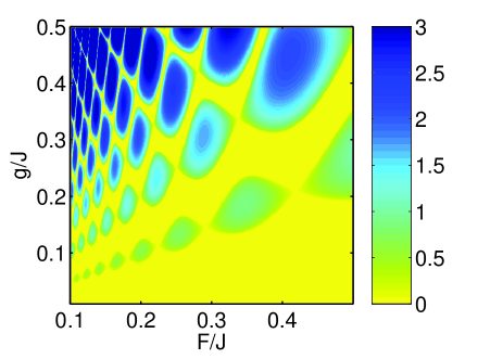
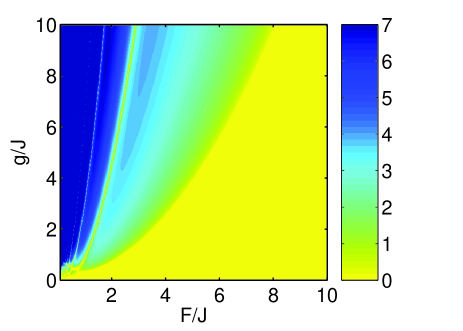
Figure 1: Increment of the dynamical (modulation) instability $\nu$ as a function of the static force magnitude $F/J$ and the interaction $g/J$ for $L=3$ sites. The yellow region in the lower panel corresponds to $\nu^{(k)}=0$ for all $k$, i.e. the Bloch oscillation is stable. A magnification of the lower left corner is depicted in the upper panel and reveals a web of additional stability regions.

As an example we show the increment of the dynamical instability for the system with only $L=3$ sites in dependence of $F/J$ and $g/J$ in Fig. 1. It is seen in the figure that the parameter space of the system is divided into two parts by a critical boundary. If the number of sites is increased, the instability regions grow and the boundary approaches approximately the curve

$$F_{cr}\approx\left\{\begin{array}[]{ll}3\,g&,\quad F<2.9\,J\\[5.69054pt] 2.96\sqrt{gJ}&,\quad F>2.9\,J\end{array}\right.$$ (15)

(see Zhen04 ). Figure 2 shows the stability diagram for $L=63$ lattice sites together with the boundary curve (15).

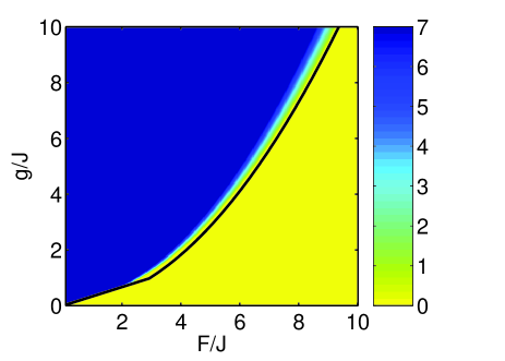
Figure 2: Same as Fig. 1 (lower panel), however for $L=63$ sites. Also shown is the boundary given by Eq. (15) as a black curve.

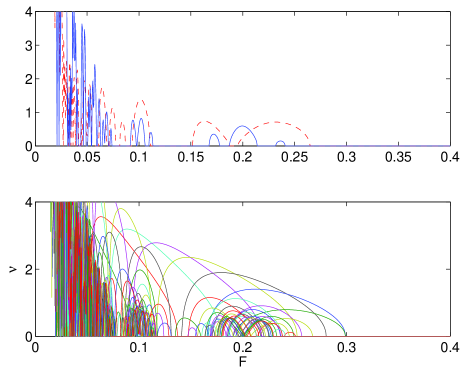
Figure 3: Increments of the modulation instability $\nu^{(k)}=\nu^{(k)}(F)$, $k=0,\,1,\ldots$ for $J=1$, $g=0.1$ and $L=5$ sites (upper panel) as well as $L=63$ sites (lower panel). With increase of the lattice size the instability regions for different $k$ overlap and cover the whole region left to the critical line.

In the right region of the diagrams $\nu=\nu(F,g)\equiv 0$ holds and BOs are always stable. Physically that means that a sufficiently large static force ensures stability even in the presence of nonlinearity. In the left hand side of the diagrams BOs are typically unstable but a closer inspection reveals a web of stability regions for smaller values of the parameters as can be seen in the upper panel in Fig. 1. It should be noted that these stability regions are a particular property of systems with a small number of lattice sites. If $L$ is increased, the regions where $\nu^{(k)}>0$ overlap (see Fig. 3) and for any point in the left side of the diagram there is at least one strictly positive increment of the dynamical instability.

II.2 Relation to chaos

In this section we investigate the implications of the stability on the dynamics of a classical ensemble of trajectories. We will address the relation between dynamical instability, classical chaos and the so-called self-thermalization, that is, equipartition of the energy between the different quasimomentum modes. Related questions have been studied in Berm84 in the context of one of the standard systems of classical chaos, the Fermi-Pasta-Ulam system FPUchaos . There it was pointed out that a positive increment $\nu$ of the dynamical instability is a necessary but not sufficient condition for the onset of developed chaos in a chain of coupled nonlinear oscillators. Here the term ‘developed chaos’ characterizes a situation where a chaotic trajectory explores the whole energy shell. Developed chaos also implies equipartition of the energy between the eigenmodes of the chain, a phenomenon often referred to as thermalization.

The consideration of an ensemble of classical trajectories as compared to a single trajectory is well suited for understanding the systems behavior in the present context for two main reasons. First it is a convenient method to capture the generic features of perturbed initial conditions due to an out-averaging of the special behavior of an individual trajectory slightly differing from the BO (10). The second reason is that the mean-field description is an approximation in the spirit of a classical limit of the many-particle system which has to be regarded as the more fundamental description. This many-particle system, however, cannot be associated with a point in the (classical) mean-field phase space, but is rather equipped with a finite width due to the uncertainty principle, where the width decreases with increasing particle number. Thus the natural counterpart of the many-particle system within the mean-field description is a phase space distribution rather than a single point. This phase space distribution can be conveniently replaced with a finite ensemble of classical trajectories for practical purposes. Further details of this considerations can be found in 07phase and Appendix B. As an example we depict in Fig. 4 the amplitudes $a_{l}$, $l=1,\ldots,L$ of an initial classical ensemble for the parameters $N=15$, $L=5$ considered in Sec. III for 100 realizations. The histograms show the corresponding probability distributions for the populations $|a_{l}|^{2}$ and the phases.

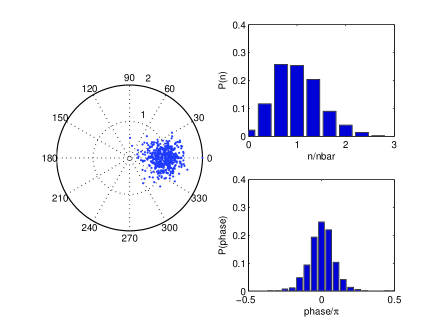
Figure 4: Classical ensemble representing the many-particle initial state for  $N=15$, $L=5$ and 100 realizations. The characteristic width of the distribution is proportional to $\bar{n}^{-1/2}$.

A convenient quantity for the characterization of the Bloch dynamics in the higher dimensional classical phase space is the classical momentum given by

$$p(t)=\frac{1}{2i}\Big{[}\sum_{l}a^{*}_{l+1}a_{l}\,e^{-iFt}-c.c.\Big{]}=\sum_{k}|b_{k}|^{2}\sin(\kappa-Ft).$$ (16)

For the periodic solution (10), that is, the BO, the momentum oscillates in a cosine manner between $-1$ and $1$ with the Bloch frequency $F$. For neighboring initial values the behavior may differ considerably, depending on the stability of the BO: If the BO is unstable we expect an exponential growth of the initial deviation connected to classical chaos, leading to thermalization. On the other hand, the naive expectation in the stable region is that a small initial deviation leads to a small deviation in the overall trajectory and therefore averaging over an ensemble does not change the Bloch oscillation behavior in principle. However, we are going to argue that this is only true in a certain range of the parameter space and indeed one can distinguish three regimes of classical motion instead of only ‘stable’ or ‘unstable’ behavior. In fact, we find that for large values of the static force $F$ the ensemble average leads to a breakdown of the BOs and even a thermalization in the absence of classical chaos.

Let us start our discussion with the unstable regime, that is, small values of $F$. The exponential growth of a deviation from the uniform initial condition is evidently related to chaos. In particular, as for the Fermi-Pasta-Ulam system FPUchaos , for the system (6) positive increments of the dynamical instability are a necessary condition for the onset of developed chaos. To illustrate the impact on the Bloch dynamics we show the time evolution for a single trajectory of an ensemble mimicking an $N=15$ particle system in Fig. 5. The first panel in the figure depicts the momentum (16) and the second panel shows the mode populations $|b_{k}(t)^{2}|$ of the quasimomentum modes $k$ as a function of time measured in units of $T_{\rm J}=2\pi/J$.

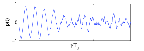
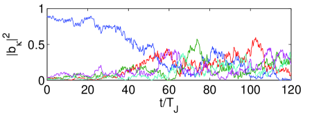
Figure 5: Mean-field BO of the momentum (upper panel) and the dynamics of the population of quasimomentum modes (lower panel). These results for a single trajectory oscillate erratically. Parameters are $L=5$, $J=1$, $g=0.1$, and $F=0.1$.

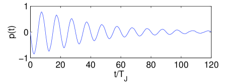
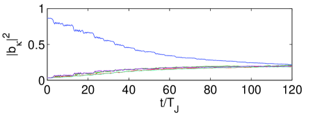
Figure 6: Mean-field BO of the momentum (upper panel) and dynamics of the populations of quasimomentum modes, averaged over an ensemble of 1000 trajectories of initial conditions (45). The other parameters are the same as in Fig. 5. An equipartition between the quasimomentum modes results in the decay of BO.

For a single run, the momentum $p(t)$ and the mode populations $|b_{k}(t)|^{2}$ start to oscillate irregularly after a transient time $t_{\nu}\sim\ln(\epsilon/\nu)$, $\epsilon\sim\bar{n}^{-1/2}$, required for the modes with $k\neq 0$ to take non-negligible values. These erratic oscillations are smoothed by averaging over the ensemble (consisting of 1000 trajectories in the present example) as shown in Fig. 6. In the ensemble average one observes a damped BO of $p(t)$ and an equipartition of the mode populations converging to the values of $1/L$, i.e., a thermalization. It is clearly seen in the figure that the rate of thermalization actually determines the decay rate of the BO. In Sec. III we will demonstrate that this (classical) mean-field dynamics agrees remarkably well with the full quantum many-particle behavior in view of the small number of three particles per site.

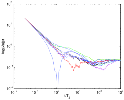
Figure 7: Finite time Lyapunov exponent $\lambda(t)$ for ten different trajectories from the ensemble (45). (Same parameters as in Fig. 5.)

One gets further insight into the relation to chaos by studying the finite time Lyapunov exponent

$$\lambda(t)=\ln|\delta{\bf a}(t)|/t\;,$$ (17)

where $\delta{\bf a}(t)$ evolves in the tangent space according to the linear equation

$$i\frac{d\delta{\bf a}}{dt}=M[{\bf a}(t)]\,\delta{\bf a}(t)$$ (18)

(see Appendix A). As an example, Fig. 7 shows the behavior of $\lambda(t)$ for ten different trajectories from an ensemble (45). It is seen that $\lambda(t)$ converges to some constant value, so that the mean Lyapunov exponent $\langle\lambda\rangle$ is a well defined quantity. Since the unstable periodic trajectory analyzed in subsection II.1 is a member of this ensemble, the maximal increment of the modulation instability $\nu={\rm max}_{k}\nu^{(k)}$ provides a reliable estimate for $\langle\lambda\rangle$. Still, because the mean Lyapunov exponent depends on the ensemble (i.e. on the value of the filling factor $\bar{n}=N/L$), generally $\langle\lambda\rangle\neq\nu$. In particular, $\langle\lambda\rangle$ is found to be a smooth function of $F$, while the maximal increment of the modulation instability is a non-analytic function of $F$ with discontinuous first derivative. As a consequence, when we cross the critical line in the stability diagram, the system shows a smooth transition from the regime of decaying BOs to the regime of persistent BOs. (For example, for the parameters of Fig. 6 this change happens in the interval $0.1\lesssim F\lesssim 0.4$.)

We now turn to the parameter regime of stable BOs, for larger values of $F$ where the increment is zero. Here we will distinguish two different types of behavior in the ensemble average: Persistent BOs for intermediate values of $F$ and decaying BOs connected to thermalization in the limit of large $F$. The regime of persistent BO is shown in Fig. 8 for an example with $F=0.4$. No energy exchange between quasimomentum modes is seen which means that the system dynamics is at least locally regular. In other words, for the considered moderate $F$ the periodic trajectory (10) is surrounded by a stability island. Moreover, the size of this stability island should be large enough as compared to the characteristic width of the distribution (45), so that the majority of the trajectories are stable. In this case, the ensemble averaging is of little influence, resulting only in a small decrease of the amplitude.

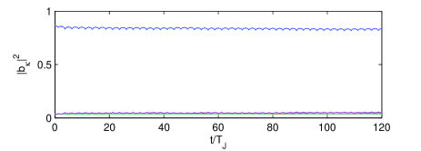
Figure 8: Same as Fig. 6, however for $F=0.4$ showing a stable Bloch oscillation.

The behavior for large values of $F$ and its relation to classical chaos is more surprising: An analysis of the phase-space structure of the system (7) reveals the volume of the regular component to grow with $F$ and for $F\rightarrow\infty$ the system becomes integrable Kolo04a . (This integrable regime has already been observed in Kolo03 .) Thus, one would first expect persisting BOs. However, the observed behavior is quite different. As an illustration we show an example for an individual trajectory in Fig. 9. Here one observes a quasiperiodic behavior. When averaged over an ensemble this leads to a decay of the BO as depicted in Fig. 10. This behavior can indeed be understood analytically. In the limit $F\to\infty$ the populations of the lattice sites are frozen and the amplitudes $a_{l}$ evolve only in the phase according to

$$a_{l}(t)\approx a_{l}(0)\exp\left[-ig(|a_{l}(0)|^{2}-1)\,t\right]\;.$$ (19)

The evolution (19) for the amplitudes $a_{l}(t)$ immediately implies the observed quasiperiodic dynamics of the amplitudes $b_{k}(t)$ (see Fig. 9). It can be shown that the decay due to the dephasing arising for the ensemble averaged dynamics obeys an $\exp(-\gamma_{r}t^{2})$-law, where the coefficient $\gamma_{r}$ is proportional to $g$ and inversely proportional to $\bar{n}$. Remarkably, the quasiperiodic dynamics also implies an equipartition between the quasimomentum modes (see Fig. 9) in the absence of classical chaos. However, there are characteristic differences compared to the decay and the thermalization processes introduced by classical chaos: First, the relaxation constant $\gamma_{r}$ for the dephasing decay depends on the characteristic width of the distribution function (45) and decreases as $1/\bar{n}$ in the semiclassical limit. On the contrary, the relaxation constant $\gamma_{c}$ for the chaotic decay decreases only as $1/\ln\bar{n}$. Second, the chaotic decay follows $\langle p(t)\rangle=\exp(-\gamma_{c}t)\sin(\omega_{B}t)$, while for the dephasing decay we have $\langle p(t)\rangle=\exp(-\gamma_{r}t^{2})\sin(\omega_{B}t)$.

Going ahead we note that both the regimes of stable BO and the one of decaying BO in the presence of classical chaos closely resemble the full many-particle dynamics when averaged over an ensemble. However, in what follows we shall find that there is an additional many-particle feature in the dynamics in the third regime of large $F$. Here the decay of the Bloch oscillations is present in the many-particle system as well and for short times the mean-field ensemble even quantitatively resembles the many-particle dynamics. However, the many-particle system shows a periodic revival behavior as already pointed out in Kolo03 which, as a pure quantum phenomenon, cannot be captured by the mean-field ensemble.

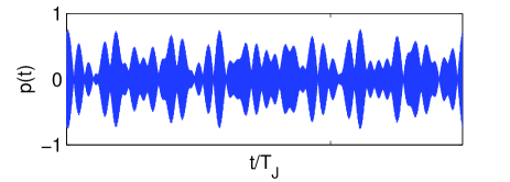
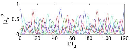
Figure 9: Same as Fig. 5, yet for $F=10$ in the strong field region.

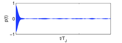
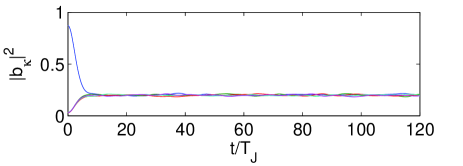
Figure 10: Same as Fig. 6, yet for $F=10$ in the strong field region.

III Many-particle dynamics

In this section we study the many-particle counterpart of the mean-field system discussed in the preceding section. This is described by the driven Bose-Hubbard Hamiltonian

$$\widehat{H}(t)=-\frac{J}{2}\sum_{l}\Big{(}e^{iFt}\hat{a}^{\dagger}_{l+1}\hat{a}_{l}+h.c.\Big{)}+\frac{W}{2}\sum_{l}\hat{n}_{l}(\hat{n}_{l}-2)\;.$$ (20)

We also confine the system to $L$ lattice sites ($L$ chosen to be odd) and apply periodic boundary conditions. Then the Hilbert space of system (20) is spanned by the Fock states $|{\bf n}\rangle=|n_{1},n_{2},\ldots,n_{L}\rangle$, where $\sum_{l}n_{l}=N$ is the total number of atoms. The dimension of the Hilbert space is equal to $\frac{(N+L-1)!}{N!(L-1)!}$ . Using the canonical transformation $\hat{b}_{k}=L^{-1/2}\sum_{l}\exp(i2\pi kl/L)\,\hat{a}_{l}$, the Hamiltonian (20) can be presented in the form

$$\widehat{H} = -J\sum_{k}\cos(\kappa-Ft)\,\hat{b}^{\dagger}_{k}\hat{b}_{k}$$ (21)

$$\ \ +\frac{W}{2L}\sum_{k_{i}}\hat{b}^{\dagger}_{k_{1}}\hat{b}_{k_{2}}\hat{b}^{\dagger}_{k_{3}}\hat{b}_{k_{4}}\,\delta_{k_{1}+k_{3},k_{2}+k_{4}}\;,$$

where we omit the constant term $W\sum_{k}\hat{b}_{k}^{\dagger}\hat{b}_{k}$. The basis vectors of the Hilbert space are now given by the Fock states in the quasimomentum representation: $|n_{-(L-1)/2},\ldots,n_{-1},n_{0},n_{+1},\ldots,n_{(L-1)/2}\rangle$ . In the coordinate representation the Fock and the quasimomentum Fock states are given by the symmetrized product of the Wannier and Bloch functions, respectively. Here we are interested in the solution of the time-dependent Schrödinger equation with the Hamiltonian (21) for initial conditions given by a BEC of atoms in the zero quasimomentum state, i.e. $|\Psi_{0}\rangle=|\ldots,0,N,0,\ldots\rangle_{q}$. This is, in fact, equivalent to an $SU(L)$ coherent state, namely

$$|\Psi_{0}\rangle=\frac{1}{\sqrt{N!}}\Big{(}\frac{1}{\sqrt{L}}\sum_{l=1}^{L}\hat{a}^{\dagger}_{l}\Big{)}^{N}\!|0\rangle=\sum_{\bf n}c_{\bf n}|{\bf n}\rangle$$ (22)

where $|{\bf n}\rangle$ with ${\bf n}=(n_{1},\ldots,n_{L})$ is a Fock state and $c_{\bf n}=\sqrt{\frac{N!}{L^{N}n_{1}!\cdots n_{L}!}}$. In general the $SU(L)$ coherent states are equivalent to the fully condensed states, where our special choice approximately corresponds to the ground state of the system at $F=0$ if the condition $W\ll J$ is satisfied.

III.1 Floquet-Bogoliubov states

First we address the question of a manifestation of the dynamical instability in the many-particle quantum system. It is argued below that, similar to the static case $F=0$, the quantum counterpart of the dynamical instability is Bogoliubov’s depletion of the condensate Legg01 . We begin with an alternative derivation of the common Bogoliubov spectrum for $F=0$ Kolo0607a which we shall then adopt to the case $F\neq 0$.

For an infinite number of particles, the Bogoliubov states can be constructed from $|\Psi_{0}\rangle$ by applying the depletion operators

$$\widehat{D}^{(k)}=\sum_{n=0}^{\infty}c_{n}^{(k)}\left(\hat{b}^{\dagger}_{-k}\hat{b}^{\dagger}_{+k}\hat{b}_{0}\hat{b}_{0}\right)^{n}\,,$$ (23)

which transfer particles from the zero quasimomentum state to the states $\pm k$ :

$$|\Psi\rangle=\prod_{k>0}\widehat{D}^{(k)}|\Psi_{0}\rangle\;.$$ (24)

In Eq. (23) the coefficients $c_{n}^{(k)}$ should be determined self-consistently so that the wave function $|\Psi\rangle$ satisfies the stationary Schrödinger equation with the Hamiltonian (21) with $F=0$,

$$\widehat{H}(F=0)|\Psi\rangle=E|\Psi\rangle\;.$$ (25)

Equations (23), (24) are equivalent to the ansatz

$$|\Psi^{(k)}\rangle=\sum_{n=0}^{\infty}c^{(k)}_{n}|..,n,..,N-2n,..,n,..\rangle_{q}\;,$$ (26)

where $n$ particles are redistributed from the zero quasimomentum state to the state $k$ and to the state $-k$. Note that here, as well as in (23), (24), the limit $N\rightarrow\infty$, $W\rightarrow 0$ with constant $g=WN/L$ is assumed, which justifies a factorization of the eigenvalue problem (25) into $(L-1)/2$ independent eigenvalue problems. Substituting the ansatz (26) into (25) and taking the above limit the original problem reduces to the diagonalization of a tridiagonal hermitian matrix $A^{(k)}$ with matrix elements

$$A^{(k)}_{n,n}=2(g+\delta)n\quad,\quad A^{(k)}_{n,n+1}=g(n+1)$$ (27)

where $\delta=J\left(1-\cos\kappa\right)$. The spectrum of the matrix $A^{(k)}$ is equidistant with a level spacing given by the Bogoliubov frequency $\Omega^{(k)}=2\sqrt{2g\delta+\delta^{2}}$. Correspondingly, the eigenvectors ${\bf c}^{(k)}$ of $A^{(k)}$ define the Bogoliubov states of the Bose-Hubbard model. It is worthwhile emphasizing that for a finite $N$ these Bogoliubov states provide only an approximation to the actual eigenstates of the Bose-Hubbard system. While this approximation can be quite accurate for the ground and low-energy states, it fails for the high-energy states Kolo0607a . The BEC depletion of these states, defined by

$$N_{D}=\sum_{k>0}\Big{(}\sum_{n=1}^{\infty}2n\,|c^{(k)}_{n}|^{2}\Big{)}\;,$$ (28)

provides a quantitative criterion for the validity of the Bogoliubov approach. Namely, if $N_{D}<<N$ then the approach is justified. On the contrary, $N_{D}\sim N$ (which is the case for high-energy states) means that the actual structure of the eigenstates has nothing to do with the presumed Bogoliubov structure (24). Furthermore, it is convenient to order the states according to the depletion (28).

Now we are in the position to discuss the case $F\neq 0$. Since we are interested in the Bloch dynamics, it is useful to introduce the evolution operator over one Bloch period 04bloch ,

$$\widehat{U}=\widehat{\exp}\Big{[}-i\int_{0}^{T_{B}}\widehat{H}(t)dt\Big{]}\;,$$ (29)

where $\widehat{H}(t)$ is given in (21) and the hat over the exponential function again denotes time ordering. We are looking for those eigenstates of $\widehat{U}$,

$$\widehat{U}\,|\Psi\rangle=\exp(-i2\pi E/F)\,|\Psi\rangle\,,$$ (30)

which have the Bogoliubov structure (24). Substituting the ansatz (26) into (30) we obtain an equation for the coefficients $c_{n}^{(k)}$:

$$\widehat{\exp}\,\Big{[}-i\int_{0}^{T_{B}}\!A^{(k)}(t)\,dt\Big{]}\,{\bf c}^{(k)}=\exp\Big{(}-i\frac{2\pi E}{F}\Big{)}\,\bf{c}^{(k)}\;,$$ (31)

where the diagonal elements of the matrix $A^{(k)}(t)$ are now given by

$$A^{(k)}_{n,n}(t)=2[\,g+\delta\cos(Ft)]n\;,\quad\delta=J(1-\cos\kappa)\;.$$ (32)

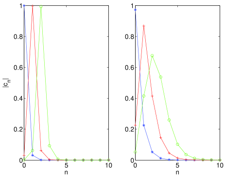
Figure 11: Left panel: Coefficients of the first three Bogoliubov states $|\Psi\rangle=\sum_{n}c_{n}|n,N-2n,n\rangle$ of the three-sites Bose-Hubbard model. Right panel: Floquet-Bogoliubov states. (Parameters $J=1$, $g=0.1$ and $F=0.4$.)

As an illustration the right panel in Fig. 11 shows the coefficients of the first three Floquet-Bogoliubov states in the quasimomentum Fock basis for $L=3$, $g=0.1$, and $F=0.4$ remarkmf1 , where the depletion is $N_{D}=0.113$, $2.341$, and $4.568$ particles, respectively. For the sake of comparison, the left panel in the figure shows the Bogoliubov states for the same value of $g=0.1$, where the depletion is $N_{D}=0.002$, $2.006$, and $4.010$. It is seen in Fig. 11 that the depletion of the driven BEC is larger than the depletion of a stationary BEC which was found to be a typical situation in further numerical studies.

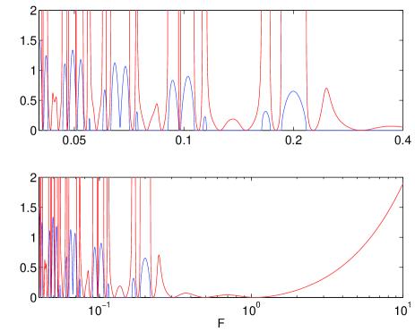
Figure 12: Number of the depleted particles $N_{D}$ (red curve) as a function of the field strength $F$ (logarithmic scale) compared to the classical increment of dynamical instability $\nu=\nu(F)$ (blue curve). Parameters are $J=1$, $g=0.1$, $L=3$. The upper panel magnifies the region of small $F$ in the lower panel.

The depletion (28) provides useful information on the BEC stability. For the ‘ground’ Floquet-Bogoliubov state the dependence $N_{D}=N_{D}(F)$ is depicted in Figs. 12 and 13. It is seen in Fig. 12 that, as a function of $F$, $N_{D}$ diverges at the points where the classical increment of the dynamical instability $\nu$ (also shown in the figure) takes positive values. (More precisely, the depletion cannot be larger than $N$. However, since the Bogoliubov theory refers to $N=\infty$, it can be formally considered as infinite.) This ‘divergence’ of $N_{D}$ means that in the regions of instability the eigenfunctions of the evolution operator differ considerably from the Bogoliubov structure. In fact, they are chaotic in the sense of quantum chaos 04bloch . It is also seen in the figure that the depletion increases linearly for $F\rightarrow\infty$. Thus the discussed Floquet-Bogoliubov states cannot be eigenstates of the evolution operator in the limit of large $F$, although the classical increments $\nu^{(k)}$ vanish identically for $F\rightarrow\infty$. We come back to this point in the next subsection.

The intervals of small depletion observed in Fig. 12 depend, of course, also on the interaction $g$. The full parameter dependence of the depletion (28) is shown in Fig. 13. For relatively low values of $g/J$ and $F/J$ (upper panel) we find a highly organized web of stability regions, whereas the behavior for larger parameters (lower panel) shows a simpler structure. These many-particle results can be directly compared with the mean-field stability diagrams in Fig. 1 which confirms the relationship between BEC depletion and mean-field stability.

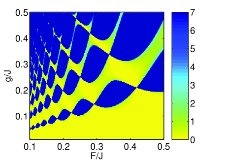
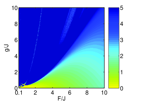
Figure 13: Number of the depleted particles $N_{D}$ as a function of the static force magnitude $F/J$ and the interaction $g/J$ for $L=3$ sites. The depletion is very small in the yellow region of the lower panel. The upper panel magnifies the lower left corner of the lower panel and reveals additional regions of small depletion.

For the sake of completeness we also briefly discuss the corresponding quasienergies $E$ (see Eq. (30)) which are defined modulo $\,\hbar\,$ times the Bloch frequency, i.e. $E_{\alpha,j}=E_{\alpha,0}+jF$, $j=0,\,\pm 1,\ldots$ . The lower panel of Fig. 14 displays the quasienergies of the five Floquet-Bogoliubov states with smallest $N_{D}$. The system parameters are $J=1$, $g=0.1$ and $L=3$ as in Fig. 12. For clarity, three Floquet zones are shown in the figure. As expected, the spectrum is equidistant with a level spacing correlated to the depletion. Note the apparent irregularity in the windows around $F=0.2$ and $F=0.17$, which is related to the region of dynamical instability of the mean-field system. For comparison, the upper panel shows the number of depleted particles $N_{D}$ as in Fig. 12 with a linearly scaled $F$-axis. In the regions of finite depletion the most stable quasienergy states appear to be very sensitive against a variation of $F$.

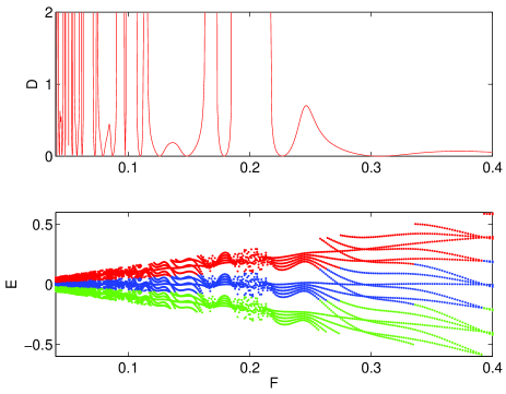
Figure 14: Lower panel: Quasienergy spectrum of the Floquet-Bogoliubov states as a function of the field strength $F$ (same parameters as in Fig. 12). Upper panel: Number of the depleted particles $N_{D}$.

III.2 Bloch oscillations

The microscopic dynamics of BOs was considered earlier in a number of papers summarized in Ref. 04bloch with focus on the regime of low filling factors $\bar{n}=N/L\leq 1$. In the present work, to make a link to the mean-field dynamics, we simulate BOs for a relatively large filling factor.

We investigate the dynamics in dependence on the force $F$ for $N=15$ and $N=20$ atoms in a lattice with $L=5$ sites. Since the plots are very similar, only the results with $N=15$ are shown. The value of the microscopic interaction constant is set to $W=0.1/\bar{n}$, so that the macroscopic interaction constant is $g=0.1$, and the hopping matrix element $J=1$. The initial wave function is chosen as the $SU(L)$ coherent state (22).

In Fig. 15 we show the dynamics of the many-particle counterpart of the mean-field quantity (16), that is, the expectation value of the many-particle momentum

$$p(t)=\frac{1}{2iN}\,\Big{\langle}\psi(t)\Big{|}\,\sum_{l}\hat{a}^{\dagger}_{l+1}\hat{a}_{l}\,e^{-iFt}-h.c.\Big{]}\Big{|}\psi(t)\Big{\rangle}$$ (33)

for $N=15$ and the three values of $F$ chosen in different dynamical regimes as shown in Figs. 6, 8 and 10.

The upper panel of Fig. 15 corresponds to $F=0.1$, which falls into the region of dynamical instability of the mean-field system. Here the quantum many-particle BO decays in very good agreement with the mean-field ensemble shown in the upper panel of Fig. 6 (note that finer details are also reproduced). This demonstrates that the ensemble averaged mean-field dynamics is capable of describing important aspects of the full many-particle system 07phase .
In the middle panel of Fig. 15 we have $F=0.4$, where the system is stable. Here the quantum many-particle BOs persist in time, also agreeing with the ensemble-averaged mean-field dynamics. As discussed above, in this regime the ensemble average is of little influence, i.e. the state is fully condensed and can be described by a single mean-field trajectory instead.

The third case, $F=10$, depicted in the lower panel of Fig. 15, requires a separate consideration. Indeed, as mentioned in the previous subsection, in the limit of large $F$ the Floquet-Bogoliubov states are not eigenstates of the evolution operator (29). Instead it can be shown that those are the Fock states $|{\bf n}\rangle$ 04bloch . Thus the time evolution of the wave function is given by

$$|\Psi(t)\rangle=\sum_{\bf n}c_{\bf n}\exp\Big{(}-i\frac{Wt}{2}\sum_{l=1}^{L}n_{l}(n_{l}-1)\Big{)}|{\bf n}\rangle\;.$$ (34)

Equation (34) implies a periodic recovering of the initial state (22) at times which are multiples of $T_{W}=2\pi/W$ and, hence, periodic revivals of BOs Kolo03 . It should be stressed that these revivals are a pure quantum many-particle effect due to the finiteness of $W$ and $\bar{n}$. This constructive interference cannot be explained within the ensemble-averaged mean-field approach. However, the breakdown can be described by the ensemble averaging and is due to dephasing, as explained in Sec. II.2.

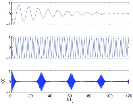
Figure 15: Bloch oscillations of $N=15$ atoms in a lattice with $L=5$ sites for $J=1$, $W=0.1/3$, and $F=0.1$ (top), $F=0.4$ (middle), and $F=10$ (bottom). Shown is the many-particle mean momentum $p(t)$ given in (33).

IV Summary

We have studied an $N$-particle system, a Bose-Hubbard Hamiltonian with linearly increasing on-site energies. This system can be conveniently reduced to a finite lattice with $L$ sites by using gauge transformation and imposing periodic boundary conditions.

Such a model can be used to describe important features of realistic systems, as for instance the dynamics of cold atoms or BECs in an optical lattice under the influence of the gravitational field Daha96 ; Raiz97 ; Ande98 ; Mors01 ; Cris02 ; Jona03 ; Ott04 ; 04bloch_bec ; Wimb05 ; Sias07 ; Gust08a ; Fatt08 , or many-particle systems in ring shaped optical lattices as proposed in Amic05 with additional driving. It should be noted, however, that it neglects a number of features. The space dimension is reduced to a quasi one-dimensional setting, a decay of the system via Zener transitions to higher bands is excluded, the lattice is discretized and truncated, and the interaction is simplified. Nevertheless, this model has been found to describe experimental results quite well. Further, the Bose-Hubbard model is of interest in its own right, as evident from the large number of studies exploring its properties which are remarkably rich.

In the present paper we have studied the Bose-Hubbard model for relatively small number of lattice sites $L\leq 5$ but relatively large number of particles up to $N=20$ to make a link with the mean-field dynamics. Our aim was twofold: First, we have demonstrated how the modulation instability observed in the mean-field system are manifested in the many-particle case. We have shown that a reasonable measure of the $N$-particle instability is provided by the quantity (28). Second, we have explored the possibility to describe the time-evolution of many-particle expectation values in terms of mean-field trajectories, averaged over an ensemble constructed from the $SU(L)$-phase space distribution of the initial many-particle state. We found that this (averaged) mean-field dynamics agrees remarkably well with the full quantum many-particle behavior in a number of cases. The only exception was the presence of many-particle revivals for strong fields which is a pure quantum phenomenon.

These observations suggest an application of the mean-field ensemble method to investigate the properties for larger lattices and larger particle numbers where many-particle computations are much more difficult or virtually impossible. Furthermore, it will be of interest to study the interrelation between classical chaotic motion and stable or decaying Bloch oscillations for more lattice sites where one can possibly make contact with recent related studies of the force free, $F=0$, case, both for the mean-field Vill00 ; Cass08 and the many-particle description Kolo0607a ; Berm04 .

Appendix A Stability Matrix

It is instructive to consider the DNLSE (6) from the viewpoint of the general theory of nonlinear dynamics. Then the solution with the initial condition $a_{l}(t=0)=1$,

$$a_{l}(t)=\exp\Big{(}i\frac{J}{F}\sin(Ft)\Big{)}\,$$ (35)

is nothing other than a periodic trajectory in a $2L$-dimensional phase space. Thus one may address the question of stability of this periodic trajectory.

Denoting by $\delta{\bf a}=(\delta a_{1},\ldots,\delta a_{L},\delta a^{*}_{1},\ldots,\delta a^{*}_{L})^{T}$ the deviation from an arbitrary trajectory ${\bf a}(t)$ and linearizing the DNLSE around this trajectory we have

$$i\,\frac{d}{dt}\delta{\bf a}=M\left[{\bf a}(t)\right]\,\delta{\bf a}\;,$$ (36)

where $M\left[{\bf a}(t)\right]$ is a $2L\times 2L$ matrix of the following structure:

$$M\left[{\bf a}(t)\right]=\left(\begin{array}[]{cc}A+gB&gC\\ -gC^{*}&-(A+gB)^{*}\end{array}\right)\;$$ (39)

$$A_{l,m}=-\frac{J}{2}\left(\delta_{l+1,m}e^{iFt}+\delta_{l-1,m}e^{-iFt}\right)\;,$$ (40)

$$B_{l,m}=|a_{l}(t)|^{2}\delta_{l,m}\;,\quad C_{l,m}=a^{2}_{l}(t)\delta_{l,m}\;.$$ (41)

Inserting the trajectory (35) into (36), the linear equation (36) takes a form where the matrix $\widetilde{M}(t)$ is periodic in time. Finally, we introduce the stroboscopic map for the discrete time $t_{n}=T_{B}n$:

$$\delta\tilde{\bf a}(t_{n+1})=U\delta\tilde{\bf a}(t_{n})\;,\quad U=\widehat{\exp}\left(-i\int_{0}^{T_{B}}\widetilde{M}(t)dt\right)\;.$$ (42)

This stability matrix $U$ is symplectic and hence the considered periodic trajectory (35) is stable if and only if all its eigenvalues lie on the unit circle.

Using the unitary transformation $U\rightarrow VUV^{-1}$, where

$$V=\left(\begin{array}[]{cc}T&0\\ 0&T\end{array}\right)\;,\quad T_{l,m}=L^{-1/2}\exp\left(\frac{i2\pi k}{L}l\right)\;,$$ (43)

the stability matrix $U$ can be factorized into $L$ decoupled $2\times 2$ matrices which can be labeled as $U^{(k)}$ with $k=0,\pm 1,\ldots,\pm(L-1)/2$. The matrix $U^{(0)}$ is not of interest here because its eigenvalues are always located on the unit circle. The explicit form of the matrix $U^{(\pm k)}$ is given by Eq. (13) and, depending on $F$, its eigenvalues $\lambda_{1,2}$ either lie on the unit circle (with $\lambda_{2}=\lambda_{1}^{*}$) or on the real axis (with $\lambda_{2}=1/\lambda_{1}$). We have stability in the first, and instability in the second case.

Appendix B Mean-Field Ensemble

Let us recall that the mean-field dynamics of the site amplitudes $a_{l}$ (or, alternatively, the quasimomentum amplitudes $b_{k}$) appears as a canonical Hamiltonian evolution in a $2L$-dimensional complex phase space which conserves the norm, i.e. the phase space is the surface of a complex sphere. In order to approximate the many-particle dynamics, we construct an ensemble of mean-field trajectories representing the initial many-body state $|\Psi(0)\rangle$. This is achieved most conveniently by using the quantum Husimi phase space distribution 07phase , the projection onto $SU(L)$ coherent states which in the quasimomentum representation is given by

$$|{\bf b}\rangle_{q}=\frac{1}{\sqrt{N!}}\,\Big{(}\sum_{k=-(L-1)/2}^{(L-1)/2}b_{k}\hat{b}_{k}^{\dagger}\Big{)}^{N}\,|0\rangle$$ (44)

with ${\bf b}=(b_{-(L-1)/2},..,b_{0},..,b_{(L-1)/2})$ and $\sum_{k}|b_{k}|^{2}=L$. For the initial many-particle state (22) this Husimi density $Q({\bf b})=|\langle{\bf b}|\Psi(0)\rangle|^{2}$ is easily calculated as

$$Q({\bf b})=B|b_{0}|^{2N},$$ (45)

where $B$ is a normalization constant. Note that the probability density for the vector components depends only on the zero-mode probability $|b_{0}|^{2}$ and is strongly localized in the region close to its maximum value $|b_{0}|^{2}=L$ for large particle number $N$.

Numerically, one can construct the ensemble (45) by means of a rejection method Pres07 : First one generates $L$ randomly distributed real numbers $r_{k}$ in the unit interval with random phases $\phi_{k}$ and normalizes the random vector with components $z_{k}=r_{k}\,e^{i\phi_{k}}$ to unity. Another random number $v$ in the unit interval is chosen in order to decide if the generated vector is accepted as a part of the ensemble: it is accepted if $v<|z_{0}|^{2N}$ and rejected otherwise. Finally we renormalize as $b_{k}=\sqrt{L}z_{k}$. If desired, the ensemble can be Fourier transformed to yield the corresponding ensemble of lattice site amplitudes $a_{l}$.

References

- (1) M. Ben Dahan, E. Peik, J. Reichel, Y. Castin, and C. Salomon, Phys. Rev. Lett. 76 (1996) 4508
- (2) M. G. Raizen, C. Salomon, and Qian Niu, Physics Today 50 (7) (1997) 30
- (3) B. P. Anderson and M. A. Kasevich, Science 282 (1998) 1686
- (4) O. Morsch, J. H. Müller, M. Cristiani, D. Ciampini, and E. Arimondo, Phys. Rev. Lett. 87 (2001) 140402
- (5) M. Cristiani, O. Morsch, J. H. Müller, D. Ciampini, and E. Arimondo, Phys. Rev. A 65 (2002) 063612
- (6) M. Jona-Lasinio, O. Morsch, M. Cristiani, N. Malossi, J. H. Müller, E. Courtade, M. Anderlini, and E. Arimondo, Phys. Rev. Lett. 91 (2003) 230406
- (7) H. Ott, E. de Mirandes, F. Ferlaino, G. Roati, G. Modugno, and M. Inguscio, Phys. Rev. Lett. 92 (2004) 160601
- (8) D. Witthaut, M. Werder, S. Mossmann, and H. J. Korsch, Phys. Rev. E 71 (2005) 036625
- (9) S. Wimberger, R. Mannella, O. Morsch, E. Arimondo, A. R. Kolovsky, and A. Buchleitner, Phys. Rev. A 72 (2005) 063610
- (10) C. Sias, A. Zenesini, H. Lignier, S. Wimberger D. Ciampini, O. Morsch, and E. Arimondo, Phys. Rev. Lett. 98 (2007) 120403
- (11) M. Gustavsson, E. Haller, M. J. Mark, J. G. Danzl, G. Rojas-Kopeinig, and H.-C. Nägerl, Physical Review Letters 100 (2008) 080404
- (12) M. Fattori, C. D’Errico, G. Roati, M. Zaccanti, M. Jona-Lasinio, M. Modugno, M. Inguscio, and G. Modugno, Physical Review Letters 100 (2008) 080405
- (13) A. R. Kolovsky and H. J. Korsch, Int. J. Mod. Phys. B 18 (2004) 1235
- (14) A. Smerzi and A. Trombettoni, Phys. Rev. A 68 (2003) 023613
- (15) M. Holthaus and S. Stenholm, Eur. Phys. J. B 20 (2001) 451
- (16) S. Mossmann and C. Jung, Phys. Rev. A 74 (2006) 033601
- (17) B. Wu and J. Liu, Phys. Rev. Lett. 96 (2006) 020405
- (18) E. M. Graefe and H. J. Korsch, Phys. Rev. A 76 (2007) 032116
- (19) X. Luo, Q. Xie, and B. Wu, Phys. Rev. A 77 (2008) 053601
- (20) M. P. Strzys, E. M. Graefe, and H. J. Korsch, New J. Phys. 10 (2008) 013024
- (21) C. Weiss and N. Teichmann, Phys. Rev. Lett. 100 (2008) 140408
- (22) A. R. Kolovsky, preprint: cond-mat/0412195 (2004)
- (23) Yi Zheng, M. Kostrun, and J. Javanainen, Phys. Rev. Lett. 93 (2004) 230401
- (24) F. Trimborn, D. Witthaut, and H. J. Korsch, Phys. Rev. A 77 (2008) 043631
- (25) A. R. Kolovsky, E. A. Gómez, and H. J. Korsch, Phys. Rev. Lett, submitted (2009) e–print arxiv:0904.4549
- (26) G. B. Berman and A. R. Kolovsky, Sov. Phys. JETP 50 (1984) 1116
- (27) See the special issue of Chaos (2005), Focus issue 15, devoted to 50-th universary of the Fermi-Pasta-Ulam problem.
- (28) A. R. Kolovsky, Phys. Rev. Lett. 90 (2003) 213002
- (29) A. J. Leggett, Rev. Mod. Phys. 73 (2001) 307
- (30) A. R. Kolovsky, New J. Phys. 8 (2006) 197; Phys. Rev. Lett. 99 (2007) 020401
- (31) In the numerical computations discussed in the following we used in most cases particles. The results are stable when is increased keeping the value of constant unless explicitely stated.
- (32) L. Amico, A. Osterloh, and F. Cataliotti, Phys. Rev. Lett. 95 (2005) 063201
- (33) P. Villain and M. Lewenstein, Phys. Rev. A 62 (2000) 043601
- (34) A. C. Cassidy, D. Mason, V. Dunjko, and M. Olshanii, arXiv.org:0805.3388 (2008)
- (35) G. B. Berman, F. Borgonovi, F. M. Izrailev, and A. Smerzi, Phys. Rev. Lett. 92 (2004) 030404
- (36) W. H. Press, S. A. Teukolsky, W. T. Vetterling, and B. P. Flannery, Numerical Recipes, Cambridge University Press, London, 3. edition, 2007